HAL Id: hal-00862645
https://hal.archives-ouvertes.fr/hal-00862645
Submitted on 30 Apr 2019
HAL is a multi-disciplinary open access
archive for the deposit and dissemination of
sci-entific research documents, whether they are
pub-lished or not. The documents may come from
teaching and research institutions in France or
abroad, or from public or private research centers.
L’archive ouverte pluridisciplinaire HAL, est
destinée au dépôt et à la diffusion de documents
scientifiques de niveau recherche, publiés ou non,
émanant des établissements d’enseignement et de
recherche français ou étrangers, des laboratoires
publics ou privés.
Multi-dimensional sparse structured signal
approximation using split bregman iterations
Yoann Isaac, Quentin Barthélemy, Cedric Gouy-Pailler, Jamal Atif, Michèle
Sebag
To cite this version:
Yoann Isaac, Quentin Barthélemy, Cedric Gouy-Pailler, Jamal Atif, Michèle Sebag. Multi-dimensional
sparse structured signal approximation using split bregman iterations. ICASSP 2013 - 38th IEEE
International Conference on Acoustics, Speech and Signal Processing, May 2013, Vancouver, Canada.
pp.3826-3830. �hal-00862645�
MULTI-DIMENSIONAL SPARSE STRUCTURED SIGNAL APPROXIMATION
USING SPLIT BREGMAN ITERATIONS
Yoann Isaac
1,2, Quentin Barth´elemy
1, Jamal Atif
2, C´edric Gouy-Pailler
1, Mich`ele Sebag
21
CEA, LIST
2TAO, CNRS
− INRIA − LRI
Data Analysis Tools Laboratory
Universit´e Paris-Sud
91191 Gif-sur-Yvette CEDEX, FRANCE
91405 Orsay, FRANCE
ABSTRACT
The paper focuses on the sparse approximation of signals using overcomplete representations, such that it preserves the (prior) structure of multi-dimensional signals. The underlying optimization problem is tackled using a multi-dimensional extension of the split Bregman optimization approach. An extensive empirical evaluation shows how the proposed ap-proach compares to the state of the art depending on the signal features.
Index Terms— Sparse approximation, Regularization, Fused-LASSO, Split Bregman, Multidimensional signals
1. INTRODUCTION
Dictionary-based representations proceed by approximating a signal via a linear combination of dictionary elements, re-ferred to as atoms. Sparse dictionary-based representations, where each signal involves but a few atoms, have been thor-oughly investigated for 1D and 2D signals for their good prop-erties, as they enable robust transmission (compressed sens-ing [1]) or image in-paintsens-ing [2]. The dictionary is either given, based on the domain knowledge, or learned from the signals [3].
The so-called sparse approximation algorithm aims at finding a sparse approximate representation of the considered signals using this dictionary, by minimizing a weighted sum of the approximation loss and the representation sparsity (see [4] for a survey). When available, prior knowledge about the application domain can also be used to guide the search toward “plausible” decompositions.
This paper focuses on sparse approximation enforcing a structured decomposition property, defined as follows. Let the signals be structured (e.g. being recorded in consecutive time steps); the structured decomposition property then re-quires that the signal structure is preserved in the dictionary-based representation (e.g. the atoms involved in the approx-imation of consecutive signals have “close” weights). The
structured decomposition property is enforced through adding a total variation (TV) penalty to the minimization objective.
In the 1D case, the minimization of the above overall ob-jective can be tackled using the fused-LASSO approach first introduced in [5]. In the case of multi-dimensional signals1 however, the minimization problem presents additional dif-ficulties. The first contribution of the paper is to show how this problem can be handled efficiently, by extending the (1D) split Bregman fused-LASSO solver presented in [6], to the multi-dimensional case. The second contribution is a com-prehensive experimental study, comparing state-of-the-art al-gorithms to the presented approach referred to as Multi-SSSA and establishing their relative performance depending on di-verse features of the structured signals.
The section 2 introduces the formal background. The pro-posed optimization approach is described in section 3.1. Sec-tion 4 presents our experimental setting and reports on the re-sults. The presented approach is discussed w.r.t. related work in section 5 and the paper concludes with some perspectives for further research.
2. PROBLEM STATEMENT
Let Y = [y1, . . . , yT] ∈ RC×T be a matrix made of T
C-dimensional signals,Φ ∈ RC×N an overcomplete dictionary
of N atoms (N > C). We consider the linear model
yt= Φxt+ et, t∈ 1, . . . , T , (1)
in which X= [x1, . . . , xT] ∈ RN×Tstands for the
decompo-sition matrix and E = [e1, . . . , eT] ∈ RC×T is a zero-mean
Gaussian noise matrix.
The sparse structured decomposition problem consists of ap-proximating the yi, i∈ {1, . . . , T } by decomposing them on the dictionaryΦ, such that the structure of the decompositions xi reflects that of the signals yi. This goal is formalized as
1Our motivating application considers electro-encephalogram (EEG)
the minimization2of the objective function min
X kY − ΦXk 2
2+ λ1kXk1+ λ2kXP k1 , (2)
where λ1and λ2are regularization coefficients and P encodes
the signal structure (provided by the prior knowledge) as in [7]. In the remainder of the paper, the considered structure is that of the temporal ordering of the signals, i.e. kXP k1 =
PT
t=2kXt− Xt−1k1.
3. OPTIMIZATION STRATEGY 3.1. Algorithm description
Bregman iterations have shown to be very efficient for ℓ1
reg-ularized problem [8]. For convex problems with linear con-straints, the split Bregman iteration technique is equivalent to the method of multipliers and the augmented Lagrangian one [9]. The iteration scheme presented in [6] considers an augmented Lagrangian formalism. We have chosen here to present ours with the initial split Bregman formulation.
First, let us restate the sparse approximation problem minX kY − ΦXk22+ λ1kAk1+ λ2kBk1
s.t. A= X B= XP
. (3)
This reformulation is a key step of the split Bregman method. It decouples the three terms and allows to optimize them sep-arately within the Bregman iterations. To set-up this iteration scheme, Eq.(3) must be transform to an unconstrained prob-lem
minX,A,B kY − ΦXk22+ λ1kAk1+ λ2kBk1
+µ1 2kX − Ak 2 2+ µ2 2 kXP − Bk 2 2 . (4) The split Bregman iterations could then be expressed as [8]
(Xi+1, Ai+1, Bi+1) = argminX,A,BkY − ΦXk22
+λ1kAk1+ λ2kBk1 (5) +µ1 2kX − A + D i Ak 2 2 +µ2 2kXP − B + D i Bk 2 2 Di+1A = Di A+ (Xi+1− Ai+1) (6) Di+1B = Di B+ (Xi+1P− Bi+1) (7)
Thanks to the split of the three terms realized above, the min-imization of Eq.(5) could be realized iteratively by alterna-tively updating variables in the system
Xi+1 = argminXkY − ΦXk22+ µ1 2kX − A i+ Di Ak 2 2 +µ2 2 kXP − B i+ Di Bk 2 2 (8)
Ai+1 = argminAλ1kAk1+µ21kXi+1− A + DiAk22 (9)
Bi+1 = argminBλ2kBk1+µ22kXi+1P− B + DiBk22(10)
2kAk p= (Pi
P
j|Ai,j|p)
1
p. The case p= 2 corresponds to the clas-sical Frobenius norm
Only few iterations of this system are necessary for conver-gence. In our implementation, this update is only performed once at each iteration of the global optimization algorithm. Eq.(9), Eq.(10) could be resolved with the soft-thresholding operator Ai+1= SoftThresholdλ1 µ1k.k1(X i+1+ Di A) (11) Bi+1= SoftThresholdλ2 µ1k.k1(X i+1P+ Di B) . (12)
Solving Eq.(8) requires the minimization of a convex differ-entiable function which can be performed via classical opti-mization methods. We proposed here to solve it determin-istically. The main difficulty in extending [6] to the multi-dimensional signals case rely on this step. Let us define H from Eq.(8) such as
Xi+1= argminXH(X) . (13)
Differentiating this expression with respect to X yields d
dXH= (2Φ
TΦ + µ
1I)X + X(µ2P PT) − 2ΦY (14)
+µ1(DAi − Ai) + µ2(DiB− Bi)PT , (15)
where I is the identity matrix. The minimum ˆX = Xi+1
of Eq.(8) is obtained by solving dXd H( ˆX) = 0 which is a Sylvester equation
W ˆX+ ˆXZ= Ci , (16)
with W = 2ΦTΦ + µ
1I, Z = µ2P PT and C = −Ui +
2ΦY + µ1Ai+ (µ2Bi− Vi)PT. Fortunately, in our case, W
and Z are real symmetric matrix. Thus, they can be diagonal-ized as follow:
W = F DwFT (17)
Z= GDzGT (18)
and Eq.(16) can then be rewritten
DwXˆ′+ ˆX′Dz= Ci′ , (19)
with ˆX′ = FTXG and Cˆ i′ = FTCiG. ˆX′is then obtained
by
∀s ∈ {1, . . . , S} ˆX′(:, s) = (Dw+ Dz(s, s)I)−1Ci′(:, s)
where the notation(:, s) indices the column s of matrices. Going back to ˆX could be performed with: ˆX= F ˆX′GT.
W and Z being independent of the iteration (i) considered, theirs diagonalization is done only once and for all as well as the computation of the terms(Dw+ Dz(s, s)I)−1 ∀s ∈
{1, . . . , S}. Thus, this update does not require heavy compu-tation. The full algorithm is summarized below.
3.2. Algorithm sum up
1: Input: Y ,Φ, P
2: Parameters: λ1, λ2, µ1, µ2, ǫ, iterM ax, kM ax
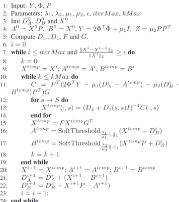
3: Init D0 A, D 0 Band X 0 4: A0 = X0 P , B0 = X0 , Y = 2ΦTΦ + µ 1I, Z= µ2P PT 5: Compute Dw, Dz, F and G. 6: i= 0
7: whilei ≤ iterM ax andkXi−Xi−1k2
kXik 2 ≥ǫ do 8: k= 0 9: Xtemp= Xi ; Atemp= Ai ; Btemp= Bi 10: whilek ≤ kM ax do 11: C = FT(2ΦTY − µ 1(DAi −Atemp) − µ2(DiB − Btemp)PT)G 12: fors → S do 13: Xtemp(:, s) = (Dy+ Dz(s, s)I)−1C(:, s) 14: end for 15: Xtemp= F XtempGT 16: Atemp= SoftThresholdλ1 µ1k.k1(X temp+ Di B) 17: Btemp= SoftThresholdλ2 µ2k.k1(X temp P+ Di B) 18: k= k + 1 19: end while 20: Xi+1= Xtemp ; Ai+1= Atemp ; Bi+1= Btemp 21: Di+1 A = D i A+ (Xi+1−Bi+1) 22: Di+1B = D i B+ X i+1 P − Ai+1) 23: i= i + 1; 24: end while 4. EXPERIMENTAL EVALUATION
The following experiment aims at assessing the efficiency of our approach in decomposing signals built with particular reg-ularities. We compare it both to algorithms coding each sig-nal separately, the Orthogosig-nal Matching Pursuit [10] and the LARS [11] (a LASSO solver) and to methods performing the decomposition simultaneously, the simultaneous OMP and FISTA [12] a proximal method solving a group-LASSO prob-lem only composed of a l1,2penalty.
4.1. Data generation
From a fixed random overcomplete dictionaryΦ, a set of K signals having piecewise constant structures have been cre-ated. Each signal is synthesized from the dictionary and a pre-determined decomposition matrix.
The TV penalization of the fused-LASSO regularization makes him more suitable to deal with data having abrupt changes. Thus, the decomposition matrices of signals have been built as linear combinations of activities. This writes as follows: Pind,m,d(i, j) = 0 if i6= ind H(j − (m −d×T 2 )) −H(j − (m + d×T 2 )) if i= k. (20)
where P ∈ RN×T, H is the Heaviside function, ind ∈
{1, . . . , N } is the index of an atoms, m is the center of the
activity and d it’s duration. A decomposition matrix X could then be written: X = M X i=1 aiPindi,mi,di (21)
where M is the number of activities appearing in one signal and ai stands for an activation weight. An example of such
signal is given in the figure (4.1) below.
Fig. 1. Built signal
4.2. Experimental setting
Each method has been applied to the previously created sig-nals. Then the distance between the decomposition matrices obtained and the real ones have been computed as follow:
dist(X, ˆX) =kX − ˆXkF kXkF
(22)
The goal was to understand the influence of the number of activities (M ) and the range of durations (d) on the effi-ciency of the fused-LASSO regularization compared to oth-ers sparse coding algorithms. The scheme of experiment de-scribed above has been carried out with the following grid of parameters:
• M ∈ {20, 30, . . . , 110}, • d ∼ U(dmin, dmax)
(dmindmax) ∈ {(0.1, 0.15), (0.2, 0.25), . . . , (1, 1)}
For each point in the above parameters grid, two set of sig-nals has been created: a train set allowing to determine for each method the best regularization coefficients and a test set designed for evaluate them with these coefficients.
Other parameters have been chosen as follows: Model Activities C= 20 m∼ U(0, T ) T = 300 a∼ N (0, 2) N= 40 ind∼ U(1, N ) K= 100
Dictionaries have been randomly generated using Gaussian independent distributions on individual elements.
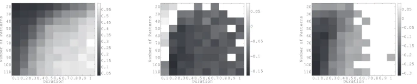
Fig. 2. Mean distances on the grid of parameters. On the left: Fused Lasso, in the middle: Fused Lasso vs LARS, on the right: Fused Lasso vs Group Lasso-Solver . The white mask corresponds to non-significant values.
4.3. Results and discussion
In order to evaluate the proposed algorithm, for each point (i, j) in the above grid of parameters, the mean of the previ-ously defined distance has been computed for each method and compared to the mean obtained by our algorithm. A paired t-test (p < 0.05) has then been performed to check the significance of these results.
Results are displayed in Figure 4.3. In the ordinate axis, the number of patterns increases from the top to the bottom and in the abscissa axis, the duration grows from left to right. The left image displays the mean distances obtained with our algo-rithm. The middle and right one present its performance com-pared to other methods by displaying the difference (point to point) of mean distances in grayscale. This difference is per-formed such that, negative values (darker blocks) means that our method outperform the other one. The white mask corre-sponds to zone where the difference of mean distances is not significant and methods have similar performances. Results of the OMP and the LARS are very similar as well as those of the SOMP and the group-Lasso solver. Thus, we only display here the matrix comparing the our method to the LARS and the group-LASSO solver.
Compared to the OMP and the LARS, our method obtains same results as them when only few atoms are active at the same time. It happens in our artificial signals when only few patterns have been added to create decomposition matrices and/or when the pattern durations are small. On the contrary, when many atoms are active simultaneously, the OMP and LARS are outperformed by the above algorithm which use inter-signal prior informations to find better decompositions. Compared to the SOMP and the group-LASSO solver, results depends more on the duration of patterns. When patterns are long and not too numerous, theirs performances is similar to the fused-LASSO one. The SOMP is outperformed in all other cases. On the contrary, the group-LASSO solver is outperformed only when patterns are short.
5. RELATION TO PRIOR WORKS
The simultaneous sparse approximation of multi-dimensional signals has been widely studied during these last years [13] and numerous methods developed [14, 15, 16, 17, 4]. More recently, the concept of structured sparsity has considered the encoding of priors in complex regularization [18, 19]. Our problem belongs to this last category with a regularisation combining a classical sparsity term and a Total Variation one. This second term has been studied intensively for image de-noising as the in the ROF model [20, 21].
The combination of these terms has been introduced as the fused-LASSO [5]. Despite its convexity, the two ℓ1
non-differentiable terms make it difficult to solve. The initial pa-per [5] transforms it to a quadratic problem and uses standard optimization tools (SQOPT). Increasing the number of vari-ables, this approach can not deal with large-scale problem. A path algorithm has been developed but is limited to the par-ticular case of the fused-LASSO signal approximator [22]. More recently, scalable approaches based on proximal sub-gradient methods [23], ADMM [24] and split Bregman itera-tions [6] have been proposed for the general fused-LASSO. To the best or our knowledge, the multi-dimensional fused-LASSO in the context of overcomplete representations has never been studied. One attempt of multi-dimensional fused-LASSO has been found in an arxiv version [7] for regression task, but the journal published version does not contain any mention of the multi-dimensional fused-LASSO anymore.
6. CONCLUSION AND PERSPECTIVES This paper has shown the efficiency of the proposed Multi-SSSA based on a split Bregman approach, in order to achieve the sparse structured approximation of multi-dimensional sig-nals, under general conditions. Specifically, the extensive val-idation has considered different regimes in terms of the sig-nal complexity and dynamicity (number of patterns simulta-neously involved and average duration thereof), and it has es-tablished a relative competence map of the proposed Multi-SSSA approach comparatively to the state of the art. Further work will apply the approach to the motivating application domain, namely the representation of EEG signals.
7. REFERENCES
[1] D.L. Donoho, “Compressed sensing,” Information The-ory, IEEE Transactions on, vol. 52, no. 4, pp. 1289– 1306, 2006.
[2] J. Mairal, M. Elad, and G. Sapiro, “Sparse represen-tation for color image restoration,” Image Processing, IEEE Transactions on, vol. 17, no. 1, pp. 53–69, 2008. [3] I. Toˇsi´c and P. Frossard, “Dictionary learning: What is
the right representation for my signal?,” Signal Process-ing Magazine, IEEE, vol. 28, no. 2, pp. 27–38, 2011. [4] A. Rakotomamonjy, “Surveying and comparing
si-multaneous sparse approximation (or group-lasso) algo-rithms,” Signal processing, vol. 91, no. 7, pp. 1505– 1526, 2011.
[5] R. Tibshirani, M. Saunders, S. Rosset, J. Zhu, and K. Knight, “Sparsity and smoothness via the fused lasso,” Journal of the Royal Statistical Society: Series B (Statistical Methodology), vol. 67, no. 1, pp. 91–108, 2005.
[6] G.B. Ye and X. Xie, “Split bregman method for large scale fused lasso,” Computational Statistics & Data Analysis, vol. 55, no. 4, pp. 1552–1569, 2011.
[7] X. Chen, S. Kim, Q. Lin, J.G. Carbonell, and E.P. Xing, “Graph-structured multi-task regression and an efficient optimization method for general fused lasso,” arXiv preprint arXiv:1005.3579, 2010.
[8] T. Goldstein and S. Osher, “The split bregman method for ℓ1regularized problems,” SIAM Journal on Imaging
Sciences, vol. 2, no. 2, pp. 323–343, 2009.
[9] C. Wu and X.C. Tai, “Augmented lagrangian method, dual methods, and split bregman iteration for rof, vecto-rial tv, and high order models,” SIAM Journal on Imag-ing Sciences, vol. 3, no. 3, pp. 300–339, 2010.
[10] Y.C. Pati, R. Rezaiifar, and PS Krishnaprasad, “Orthog-onal matching pursuit: Recursive function approxima-tion with applicaapproxima-tions to wavelet decomposiapproxima-tion,” in Sig-nals, Systems and Computers, 1993. 1993 Conference Record of The Twenty-Seventh Asilomar Conference on. IEEE, 1993, pp. 40–44.
[11] B. Efron, T. Hastie, I. Johnstone, and R. Tibshirani, “Least angle regression,” The Annals of statistics, vol. 32, no. 2, pp. 407–499, 2004.
[12] A. Beck and M. Teboulle, “A fast iterative shrinkage-thresholding algorithm for linear inverse problems,” SIAM Journal on Imaging Sciences, vol. 2, no. 1, pp. 183–202, 2009.
[13] J. Chen and X. Huo, “Theoretical results on sparse rep-resentations of multiple-measurement vectors,” Signal Processing, IEEE Transactions on, vol. 54, no. 12, pp. 4634–4643, 2006.
[14] J.A. Tropp, A.C. Gilbert, and M.J. Strauss, “Algorithms for simultaneous sparse approximation. part i: Greedy pursuit,” Signal Processing, vol. 86, no. 3, pp. 572–588, 2006.
[15] J.A. Tropp, “Algorithms for simultaneous sparse ap-proximation. part ii: Convex relaxation,” Signal Pro-cessing, vol. 86, no. 3, pp. 589–602, 2006.
[16] R. Gribonval, H. Rauhut, K. Schnass, and P. Van-dergheynst, “Atoms of all channels, unite! average case analysis of multi-channel sparse recovery using greedy algorithms,” Journal of Fourier analysis and Applica-tions, vol. 14, no. 5, pp. 655–687, 2008.
[17] S.F. Cotter, B.D. Rao, K. Engan, and K. Kreutz-Delgado, “Sparse solutions to linear inverse problems with multiple measurement vectors,” Signal Processing, IEEE Transactions on, vol. 53, no. 7, pp. 2477–2488, 2005.
[18] J. Huang, T. Zhang, and D. Metaxas, “Learning with structured sparsity,” Journal of Machine Learning Re-search, vol. 12, pp. 3371–3412, 2011.
[19] R. Jenatton, J.Y Audibert, and F. Bach, “Structured vari-able selection with sparsity-inducing norms,” Journal of Machine Learning Research, vol. 12, pp. 2777–2824, 2011.
[20] L.I. Rudin, S. Osher, and E. Fatemi, “Nonlinear total variation based noise removal algorithms,” Physica D: Nonlinear Phenomena, vol. 60, no. 1-4, pp. 259–268, 1992.
[21] J. Darbon and M. Sigelle, “A fast and exact algorithm for total variation minimization,” Pattern recognition and image analysis, pp. 717–765, 2005.
[22] H. Hoefling, “A path algorithm for the fused lasso signal approximator,” Journal of Computational and Graphi-cal Statistics, vol. 19, no. 4, pp. 984–1006, 2010. [23] J. Liu, L. Yuan, and J. Ye, “An efficient algorithm for
a class of fused lasso problems,” in Proceedings of the 16th ACM SIGKDD international conference on Knowl-edge discovery and data mining. ACM, 2010, pp. 323– 332.
[24] B. Wahlberg, S. Boyd, M. Annergren, and Y. Wang, “An admm algorithm for a class of total variation regularized estimation problems,” arXiv preprint arXiv:1203.1828, 2012.