HAL Id: hal-01759922
https://hal.archives-ouvertes.fr/hal-01759922
Submitted on 6 Apr 2018
HAL is a multi-disciplinary open access
archive for the deposit and dissemination of
sci-entific research documents, whether they are
pub-lished or not. The documents may come from
teaching and research institutions in France or
abroad, or from public or private research centers.
L’archive ouverte pluridisciplinaire HAL, est
destinée au dépôt et à la diffusion de documents
scientifiques de niveau recherche, publiés ou non,
émanant des établissements d’enseignement et de
recherche français ou étrangers, des laboratoires
publics ou privés.
3D reconstruction of dynamic liquid film shape by
optical grid deflection method
L. Fourgeaud, E. Ercolani, J. Duplat, P. Gully, Vadim Nikolayev
To cite this version:
L. Fourgeaud, E. Ercolani, J. Duplat, P. Gully, Vadim Nikolayev. 3D reconstruction of dynamic liquid
film shape by optical grid deflection method. European Physical Journal E: Soft matter and biological
physics, EDP Sciences: EPJ, 2018, 41, pp.22 - 29. �10.1140/epje/i2018-11611-2�. �hal-01759922�
L. Fourgeaud , E. Ercolani , J. Duplat , P. Gully and V. S. Nikolayev 1
PSA, Route de Gisy, 78140 V´elizy-Villacoublay, France
2
Universit´e Grenoble Alpes, CEA, INAC, Service des Basses Temp´eratures, 38000 Grenoble, France
3
Service de Physique de l’ ´Etat Condens´e, CEA, CNRS, Universit´e Paris–Saclay, CEA Saclay, 91191 Gif-sur-Yvette Cedex, France
Received: / Revised version:
Abstract. In this paper, we describe the optical grid deflection method used to reconstruct 3D profile of liquid films deposited by a receding liquid meniscus. This technique uses the refractive properties of the film surface and is suitable for liquid thickness from several microns to millimeter. This method works well for strong interface slopes and changing in time film shape; it applies when the substrate and fluid media are transparent. The refraction is assumed to be locally unidirectional. The method is particularly appropriate to follow the evolution of parameters such as dynamic contact angle, triple liquid-gas-solid contact line velocity or dewetting ridge thickness.
PACS. XX.XX.XX No PACS code given
Introduction
Dynamics of dewetting films, spreading drops and moving triple liquid-gas-solid contact lines can be assessed with various experimental methods. Most of those are optical techniques which are suitable for studying interface move-ment because they are non-intrusive and do not disturb the fluid. We present here a method we used to accu-rately measure the temporal evolution of the topography of evaporating liquid films.
The idea is to obtain local properties of a heteroge-neous medium by measuring the visible displacement of the object points created by the light refraction in the medium. To our knowledge, this principle has been first proposed by Kurata et al. [1] to measure the deformation of a water interface and by Gurfein et al. [2] to characterize spatial variations of the refraction index of a thin trans-parent fluid layer. In [2], the parallel light rays crossed first the fluid layer and were refracted by it. Then the light fell to a grid of parallel wires situated close to this cell so that both were in focus of a camera behind. The grid image displacement in the direction perpendicular to it was proportional to the gradient of the fluid refraction index in the same direction. A similar setup has been used by Hegseth et al. [3] who have adapted it to observe the liquid film shape in a space-based experiment. Incident light rays were refracted at the film surface and the grid image distortion gave information about the film
thick-a
Present address: Mechanical Design Office, Airbus Defence and Space, 31 rue des Cosmonautes, 31402 Toulouse Cedex 4, France
ness. However the precision was weak for several reasons; in particular, the grid was out of focus.
In a setups used by Kurata et al. and Andrieu et al. [4], a square grid pattern was drawn with an ink at the bottom of a thick transparent solid substrate. The lat-ter was backlit with a diffuse light and the liquid droplet is placed at the top. The camera was situated above the droplet, far away from it. The light rays were refracted at the liquid air interface and the grid image was distorted. The authors suggested measuring the grid distortion very close to the contact line to obtain the contact angle in dy-namics. As one will see below, this method lacks precision when the slopes become large because one cannot mea-sure the displacement at the contact line (only at some distance from it). In the works of Banaha et al. [5] and Kajiya et al. [6], a grid projection method has been used to track the contact line position of a water droplet on gels and to measure the droplet profile.
More recently, the grid was suggested to be replaced by a randomly placed points pattern [7]. This method works well for small surface slopes and does not require any sup-plementary information (unlike the grid method as we will explain later) on the direction of the local film slope. The method however does not expect to work at large slopes (like those in the contact line vicinity) where the points would need to be placed densely so the correspondence between the object and image points is difficult to be es-tablished.
Snoeijer et al. [8] have used a single wire to reconstruct the 2D film profile. Unlike other experiments, they have placed the light source and the camera at the same side of
2 L. Fourgeaud et al.: 3D reconstruction of dynamic liquid film shape by optical grid deflection method
Fig. 1. General scheme of the optical grid deflection technique setup.
the fluid interface and used the wire reflection in the mir-ror polished substrate surface so the light ray is refracted twice by the film surface.
The main objective of the described setup is the 3D shape reconstruction of liquid films with contact lines. Such a reconstruction allows to determine precisely the local apparent contact angles, which is necessary to un-derstand the contact line motion (i.e. drying) dynamics.
Fluid cell
Fig. 1 presents the optical setup that is most appropriate for our case. The light source put behind the fluid cell is diffuse. The grid is placed between the source and the cell. The distance dg between the liquid film and the grid
controls the grid deflection and for this reason needs to be adjustable. A video camera is set up far from the cell so that the lens collects the parallel light rays. A square patterned grid [4] is not required; the grid with inclined parallel threads is used to reduce the image treatment complexity. The grid inclination (45◦ with respect to the
vertical axis) is chosen in such a way that it is never par-allel to the contact line.
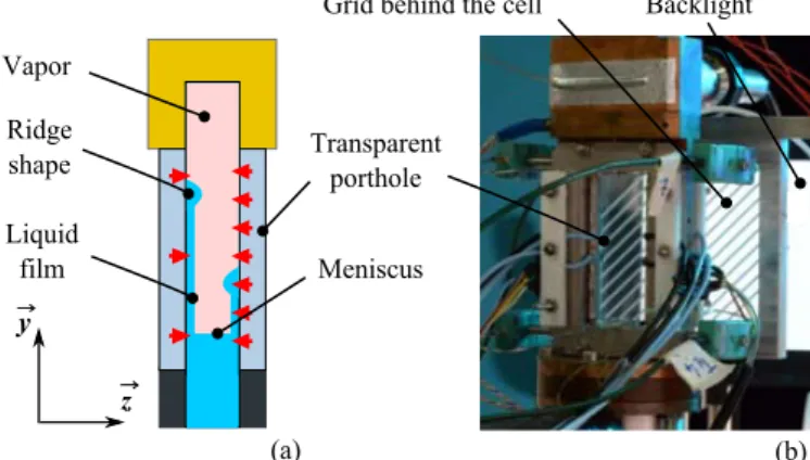
The fluid cell is a vertical closed Hele-Shaw cell made of two parallel sapphire portholes separated by gap of the spacing dc= 2 mm (Fig. 2). Inside the cell, a liquid
menis-cus of ethanol oscillates in its pure vapor atmosphere. During its receding, the meniscus deposits a liquid film on both portholes. These portholes are heated thanks to ITO (indium-tin oxide) transparent resistive layers. The back porthole is heated stronger than the other so the film deposited on it evaporates quicker and the front film (camera side) can be investigated alone.
The grid is formed by ceramic (alumina 99.9 %) threads of rectangular cross-section of 2 mm thickness in the im-age (i.e. xy) plane. They are straight because of their rigidity and have regular and sharp edges. The threads are equally spaced due to the high precision machining of the aluminum frame. As the distortion near the con-tact line is strong, the number of threads is limited in order to prevent an overlap between the distorted and non-distorted threads. The light source is a white light LED panel (50000 cd/m2). The video camera is equipped
Fig. 2. (a) Scheme of the experimental cell cross-section and (b) its photo.
with a CMOS 2/300 sensor of resolution 2048×1088. As
the film oscillation frequency is 1.5 Hz, the camera is used with the frame rate of 280 images per second.
2D film deformation
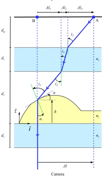
To explain the film shape reconstruction, let us assume first that the film is deformed along a single direction l, i.e. that its deformation is 2D (Fig. 3). An incident light ray is refracted by several interfaces. Point A is the object point at the grid thread; point B is its image viewed by the video camera. α is the angle of the tangent to the film and h = h(l) is its local thickness. dg and dsrepresent the
distance between the grid and the cell and the thickness of substrate, respectively.
The camera situates far from the cell and its lens is focused at infinity; we assume that the collected rays are parallel to the optical axis. As the porthole plane (i.e. the film substrate) is perpendicular to the optical path, the ray is not refracted at its interfaces. The last refraction occurs at the film interface as shown in Fig. 3.
The ray deflection from point A to point B is denoted ∆l = lA− lB. One applies the refraction law at each
inter-face. Angles are oriented positively in the trigonometric direction. The refractive indexes of the ethanol vapor and of the air are both equal to 1. In the liquid ethanol and in the sapphire substrate, refractive indexes are respectively nl= 1.355 and ns= 1.78. On the film free surface:
sin(i1) = nlsin(α). (1)
On the interface vapor/substrate and substrate/air: sin(i2) = nssin(i3), (2)
where i2 = i1− α (Fig. 3). Deflections created in each
medium read:
∆l1= (dc− h) tan(i2) (3)
= ' dctan(i2) (4)
∆l2= dstan(i3) (5)
Fig. 3. Ray tracing in the plane (l,z) orthogonal to the triple contact line and to the porthole plane. In reality, dg is much
larger than both ds and dc, and dc= ds.
The total deflection ∆l is a sum of three contributions, ∆l = ∆l1+ ∆l2+ ∆l3 (7)
The last contribution is the largest, ∆l3 ∆l1+ ∆l2,
because dg = 6 cm while dc = ds = 2 mm. Eqs. (1) and
(2) serve to express ∆l as a function of the angle α, ∆l ' dgtan (arcsin(nlsin α) − α) . (8)
As nl > 1, ∆l is of the same sign as α. Knowing ∆l,
numerical solution of Eq. (8) gives the angle α. Since α is defined in the Cartesian reference (l, z),
dh
dl = tan α, (9) where l is the coordinate of the point B associated to the l axis. The integration of this last equation leads to h as a function of l.
3D reconstruction
To reconstruct the film profile, one needs to determine a unique object point A corresponding to each point B of the grid image. This is however not trivial when the film thickness h depends both on x and y. In this case the direction l of Fig. 3 is that of the gradient of h (i.e., the steepest slope direction that varies in space). However one cannot determine the direction l for each point Bi from
the image because the grid threads are continuous; one needs an additional information or hypothesis.
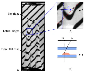
Fig. 4a presents a typical image of our cell. The trape-zoidal film shape is common in the capillary dewetting of the flat surface [8, 9]. In the present case, the substrate is heated above the saturation temperature so the film evap-oration occurs. The origin of the dewetting phenomenon observed at evaporation is explained in our preceding ar-ticle [10]. While the overall evaporation is weak, the evap-oration mass flux varies sharply over the film area. The evaporation rate is especially strong near the contact line [11, 12], which creates high apparent contact angles [13] in spite of the complete wetting conditions at equilibrium. The high contact angle, in its turn, causes the capillary dewetting phenomenon and a ridge-like structure along the contact line (cf. Fig.2a) similarly to the non-wetting situation with no evaporation [8].
Because of the high thermal conductivity of sapphire, its temperature is nearly homogeneous. This means that the evaporation is nearly invariable along the contact line, which is thus straight with the ridge profile invariable along it. Indeed, one can see in Fig. 4a that the ridge zone width variation along the contact line is small. In the ridge zone one can thus assume a 2D film profile in the direction orthogonal to the contact line (associated with the l axis) by neglecting the film slope in the direc-tion tangential to the contact line. In other words, h will be assumed to depend only on |l|, and not on the coordi-nate on the direction tangential to the contact line. The validity of such an assumption will be evaluated below.
In Fig. 4b, the red line represents the contour of the object thread. The blue arrow shows the deflection ∆l created along the l axis shown in black. The schematized cross section along the l axis is represented in Fig. 4c.
The direction of the axis l may vary from one image point to another. In Fig. 4, three zones where the contact line is straight can be distinguished: on the top ridge zone, the contact line is horizontal; on the lateral ridge zones, it is inclined with respect to y direction. Consequently, it
4 L. Fourgeaud et al.: 3D reconstruction of dynamic liquid film shape by optical grid deflection method
Fig. 4. (a) Different zones of the film on the film image. (b) Zoom on the lateral ridge. (c) Ridge cross-section corrrespond-ing to the image (b).
is possible to define only three different l directions corre-sponding to each ridge zone (Fig. 5). Note that the thread images are not deflected in the central zone. This means that the liquid film does not refract the light there and thus is nearly flat [14].
Definition of the axes
From Fig. 4, we define a Cartesian reference (x, y). The x axis is oriented from left to right and vector y from bottom to top (Fig. 5). The origin of this reference system situates at the image left-bottom corner. For each ridge zone, we define also a basis (l, z) belonging to the plane orthogonal to the contact line. Vector l belongs to the plane (x, y). It is oriented inside the liquid film in agreement with Fig. 3. Vector z is orthogonal to the plane (x, y) and is oriented from the outside to the inside of the cell (Fig. 5) so that h > 0. It gives the direction of optical axis. Besides, both lateral parts of the ridge are inclined. Their contact lines are assumed to be straight (as discussed above) and form angles ϕland ϕrwith x. In the following, these angles will
be denoted ϕj ≥ 0, j can take the value l, r, t to refer to
the left, right or top ridge zone.
The direction l depends on the considered image point Bi. The unit vector along it is defined as el= (sin ϕl, − cos ϕl)
for the left side, el= (− sin ϕr, − cos ϕr) for the right side
and e = (0, −1) for the top side.
Deflection calculation
The set of Eqs 8 and 9 is sufficient to obtain the 3D profile h(l) once the displacement ∆l is known. Fig. 6 illustrates the geometrical construction to obtain ∆li for a point Bi
which is the image of the point Ai. Point Ci is the
verti-cal projection of point Bi onto the reference thread. The
distance between points Bi and Ci is ∆yi = yB− yC.
Fig. 5. Definition of the axes to study each ridge zone.
Fig. 6. Geometrical scheme of deflection at the lateral left (cf. Fig. 4b for the corresponding image) and right parts of the ridge, respectively.
We introduce βl = β and βr = −β according to the
ridge part. In the following, it will be merely noted βjwith
j = {l, r}. Whatever the observed side, the sine theorem applied to the triangle ABC gives
1 ∆li sin(π 2 − β) = 1 ∆yi sin(γ) (10) We note that γ = π 2 − ϕj+ βj. According to Eq. (10), ∆li = cos(β) cos(βj− ϕj) ∆yi (11)
Finally, by measuring the distance ∆yi, one deduces ∆li
from Eq. (11). For the top ridge part,
∆li = ∆yi. (12)
∆yican be measured on film pictures. Thanks to Eq. (11)
and (12), ∆li is deduced from ∆yi. And ∆yi is then used
in Eq. (8) to obtain the αi angle for each point of the
li =
−−−→ B1Bi.el
= (xi− x1) sin ϕl− (yi− y1) cos ϕl. (13)
On the right side we obtain (by definition of points B1 et
BN):
li=
−−−→ BNBi.el
= −(xi− xN) sin ϕr− (yi− yN) cos ϕr. (14)
On the top ridge part:
li= yN− yi. (15)
By knowing li abscissa for each point of the distorted
perimeter, one discretizes Eq. (9). Integration is performed from the film center (where the initial condition is given by the measured by interferometry film thickness hc as
explained below) towards the edges. We note that l1 =
lN= 0. On the left side:
hi−1= (li−1− li)
tan αi+ tan αi−1
2 + hi. (16) On the right and top parts, the formula is different, be-cause the points numbering is performed in the opposite to l direction:
hi+1 = −(li+1− li)
tan αi+ tan αi+1
2 + hi. (17) We note that the film thickness hi is determined at the
points Bi (xi, yi) (i.e. along the distorted image of the
thread) and not at the points Ai (along the straight
refer-ence thread line). The film points (xi, yi, hi) are obtained
for both the upper and the lower thread borders. Typical 3D profiles are presented below: Fig. 7 shows the evolution of the film at three time moments. The 3D reconstruction of each picture is given in Fig. 8.
Infine, every thickness points obtained are plotted on the same graph in 3D (blue dotted lines on Fig 8). The 3D reconstruction is completed by using interpolation (col-ored meshes).
Thickness of the central film part
The central film part is flat. In fact the film slope exists, but is very small, of the order of 0.6◦[14]. Because of this,
its thickness hc can be measured by the Ocean Optics
Fig. 7. Film images at different time moments.
HR2000+ spectrometer with a probe that integrates both white light emitting and light sensor parts. If illuminated normally to its surface, the film forms a kind of Fabry-Perot interferometer. The rays that are reflected at the cell-liquid and liquid-vapor interfaces interfere and the re-sulting spectrum is analyzed by the device. The spectrum maxima occur when the phase difference
∆φ ≡ 2π λm
p = 2πm (18)
with
p = 2nlhc, (19)
the optical path difference, m, an arbitrary integer num-ber, and λm, the corresponding wavelength of the
spec-trum maximum. From Eq. (18), one obtains λ−1
m = m/p.
By plotting the inverse wavelengths of the spectrum max-ima versus their consecutive numbers, one thus obtains a straight line. The film thickness can be inferred from the slope with Eq. (19). This leads to the film thickness value just in front of the probe. As the interferometer time response is small enough (10 ms) with respect to the film oscillation period (0.5 s), the thickness is known in real time. This measurement is synchronized with the im-age acquisition, and all the data are combined to achieve the final reconstruction. The measurement uncertainty has been evaluated to be ± 3 µm by using different samples of known thickness.
Apparent contact angle
It is difficult to reconstruct the film profile in the con-tact line vicinity and an extrapolation is needed to obtain the contact angle with a sufficient precision. From pre-vious studies [8, 15, 16], we know that the ridge should be a cylindrical segment; our data confirm that it is so (Fig. 10). It is thus possible to fit the ridge reconstruction
6 L. Fourgeaud et al.: 3D reconstruction of dynamic liquid film shape by optical grid deflection method
Fig. 8. 3D film shape reconstruction from the respective im-ages shown in Fig 7.
with a circle. The extrapolation of circle allows us deter-mining the contact angle θapp between the ridge and the
substrate as shown in Fig. 10, θapp= arccos
z
r, (20)
with z the height of the circle center with respect to the substrate surface and r the circle radius.
Error bar
The optical grid deflection method has been validated thanks to prisms of known in advance angles. The influ-ence of refractive indexes (of liquid ethanol and sapphire) and the accuracy of grid contour detection have been es-timated: the global uncertainty on the α angle is ± 2◦.
However, the dominant error source seems to be the hypothesis about the absence of the film slope in the di-rection tangential to the contact line. In reality, the ridge
0 0.5 1 1.5 2 0 50 100 150 200 x (cm) h (µ m)
Fig. 9. Film cross section at the height y = 3 cm from Fig. 8 along x. Dotted lines: left and right parts of the ridge fitted with a circle. Note the scale difference between x and y-axis that causes the circle deformation. For this case, θapp= 9◦.
Fig. 10. Geometrical construction used to deduce the appar-ent contact angle θapp. The flat film area and the ridge are
represented in blue; the osculating circle is dotted.
is somewhat larger at the bottom compared to the top. This can be seen in Fig. 7. The related error can be evalu-ated as follows. The resulting ridge thickness uncertainty is noted δh and is proportional to the ridge thickness vari-ation δL, let us say on a scale of the total height δy of the film. From Eq. (9),
δh = δL tan(α) (21) where α is the value averaged over the ridge. δL is related to δy,
δL = δyLb− Lt yt− yb
, (22)
where Lb is the ridge width at the film bottom yb and Lt
is the ridge width at the film top yt. Over the total film
height, the global error does not exceed ± 10%.
Conclusion
The grid deflection method described here is based on the light refraction at the strongly curved liquid film surface. It is possible to provide the 3D reconstruction of a curved interface provided that the direction of maximum slope is known, which is the case of the liquid ridge observed e.g. in dewetting liquid films. The method is non-intrusive. The
out this project. We are grateful to B. Andreotti for his advice concerning the film thickness measurements and to D. Garcia and F. Bancel for their help. We thank V. Padilla for machining the grid frame. The financial con-tributions of ANR within the project AARDECO ANR-12-VPTT-005-02, of CNES within the “Fundamental and applied microgravity” program and of ESA within MAP INWIP are acknowledged.
Author contribution statement
All authors contributed to this study. LF, EE, PG con-tributed to the development of experimental installation. LF, JD and EE conducted the experiment. LF, VN and JD developed the theory of 3D reconstruction and analyzed the results of experiments. LF and VN have prepared the manuscript, with input from all other authors.
References
1. J. Kurata, K.T.V. Grattan, H. Uchiyama, T. Tanaka, Rev. of Sci. Instr. 61, 736 (1990)
2. V. Gurfein, D. Beysens, Y. Garrabos, B.L. Neindre, Optics Comm. 85, 147 (1991)
3. J. Hegseth, A. Oprisan, Y. Garrabos, V.S. Nikolayev, C. Lecoutre-Chabot, D. Beysens, Phys. Rev. E 72, 031602 (2005)
4. C. Andrieu, D. Chatenay, C. Sykes, C. R. Acad. Sci., Ser. IIb 320, 351 (1995)
5. M. Banaha, A. Daerr, L. Limat, Eur. Phys. J. Special Topics 166, 185 (2009)
6. T. Kajiya, A. Daerr, T. Narita, L. Royon, F. Lequeux, L. Limat, Soft Matter 7, 11425 (2011)
7. F. Moisy, M. Rabaud, K. Salsac, Exp. Fluids 46, 1021 (2009)
8. J.H. Snoeijer, G. Delon, M. Fermigier, B. Andreotti, Phys. Rev. Lett. 96, 174504 (2006)
9. P. Gao, L. Li, X.Y. Lu, Phys. Rev. E 91, 023008 (2015)
10. L. Fourgeaud, E. Ercolani, J. Duplat, P. Gully, V.S. Nikolayev, Phys. Rev. Fluids 1, 041901 (2016) 11. P.C. Wayner, Y.K. Kao, L.V. LaCroix, Int. J. Heat
Mass Transfer 19, 487 (1976)
12. R. Raj, C. Kunkelmann, P. Stephan, J. Plawsky, J. Kim, Int. J. Heat Mass Transfer 55, 2664 (2012) 13. V. Janeˇcek, V.S. Nikolayev, Europhys. Lett. 100,