Mixing, transport and turbulence modulation in solid suspensions : study and modelling

(1)

HAL Id: tel-01534441

https://tel.archives-ouvertes.fr/tel-01534441

Submitted on 7 Jun 2017

HAL is a multi-disciplinary open access archive for the deposit and dissemination of sci-entific research documents, whether they are pub-lished or not. The documents may come from teaching and research institutions in France or abroad, or from public or private research centers.

L’archive ouverte pluridisciplinaire HAL, est destinée au dépôt et à la diffusion de documents scientifiques de niveau recherche, publiés ou non, émanant des établissements d’enseignement et de recherche français ou étrangers, des laboratoires publics ou privés.

suspensions : study and modelling

François Laenen

To cite this version:

François Laenen. Mixing, transport and turbulence modulation in solid suspensions : study and modelling. Other [cond-mat.other]. Université Côte d’Azur, 2017. English. �NNT : 2017AZUR4010�. �tel-01534441�

(2)

Université Côte d’Azur

École doctorale de Sciences Fondamentales et Appliquées

Unité de recherche :

Laboratoire Joseph-Louis Lagrange – UMR 7293

Thèse de doctorat

Présentée en vue de l’obtention du

grade de Docteur en Sciences de

Université Côte d’Azur

Discipline : Physique

Présentée et soutenue par

François Laenen

Mixing, transport and turbulence

modulation in solid suspensions

Study and modelling

Dirigée par Jérémie Bec, Directeur de Recherche CNRS, Observatoire de la

Côte d’Azur et codirigée par Giorgio Krstulovic, Chargé de Recherche CNRS,

Observatoire de la Côte d’Azur

Soutenue le 24 février 2017 Devant le jury composé de :

Sergio Chibbaro Maitre de Conférence HDR, Université Pierre et Marie Curie Rapporteur

Romain Volk Maitre de Conférence HDR, ENS Lyon Rapporteur

Guido Boffetta Professeur, Université de Turin, Italie Examinatrice

Aurore Naso CR CNRS, Ecole centrale Lyon Examinatrice

Mikhael Gorokhovski Professeur, Ecole centrale Lyon Examinateur

Emmanuel Villermaux Professeur, Aix-Marseille Université Examinateur

Jérémie Bec DR CNRS, Université Côte d’Azur Directeur

(3)

Summary

The transport of particles by turbulent flows is ubiquitous in nature and industry. It occurs in planet formation, plankton dynamics and combustion in engines. For the dispersion of atmospheric pollutants, traditional predictive models based on eddy diffusivity cannot accurately reproduce high concentration fluctuations, which are of primal importance for ecological and health issues.

The first part of this thesis relates to the dispersion by turbulence of tracers continuously emitted from a point source. Mass fluctuations are characterized as a function of the distance from the source and of the observation scale. The combination of various physical mixing processes limits the use of fractal geometric tools. An alternative approach is proposed, allowing to interpret mass fluctuations in terms of the various regimes of pair separation in turbulent flows.

The second part concerns particles with a finite and possibly large inertia, whose dispersion in velocity requires developing efficient modelling techniques. A novel numerical method is proposed to express inertial particles distribution in the position-velocity phase space. Its convergence is validated by comparison to Lagrangian measurements. This method is then used to describe the modulation of two-dimensional turbulence by large-Stokes-number heavy particles. At high inertia, the effect is found to be analogous to an effective large-scale friction. At small Stokes numbers, kinetic energy spectrum and nonlinear transfers are shown to be modified in a non trivial way which relates to the development of instabilities at vortices boundaries.

R´

esum´

e

Le transport de particules par des écoulements turbulents est un phénomène présent dans de nom-breux écoulements naturels et industriels, tels que la dispersion de polluants dans l’atmosphère ou du phytoplancton et plastiques dans et à la surface des océans. Les modèles prédictifs classiques ne peuvent prévoir avec précision la formation de larges fluctuations de concentrations.

La première partie de cette thèse concerne une étude de la dispersion turbulente de traceurs émis `

a partir d’une source ponctuelle et continue. Les fluctuations spatiales de masse sont déterminées en fonction de la distance à la source et à l’échelle d’observation.

La combinaison de plusieurs phénomènes physiques à l’origine du mélange limite la validité d’une caractérisation de géométrie fractale. Une approche alternative est proposée, permettant d’interpréter les fluctutations massiques en terme des différents régimes de séparation de pair dans des écoulements turbulents.

La seconde partie concerne des particules ayant une inertie finie, dont la dispersion dans l’espace des vitesses requiert de développer des techniques de modélisation adaptées. Une méth-ode numérique originale est proposée pour exprimer la distribution des particles dans l’espace position-vitesse. Cette méthode est ensuite utilisée pour décrire la modulation de la turbulence bi-dimensionnelle par des particules inertielles. A grand nombres de Stokes, l’effet montré est ana-logue à celui d’une friction effective à grande échelle. Aux petits Stokes, le spectre de l’énergie cinétique du fluide et les transferts non-linéaires sont modifées d’une manière non triviale.

(4)

Nomenclature

V Tracer velocity.

Vp Inertial particle velocity.

X Tracer position.

Xp Inertial particle position.

xS Position of the injecting source.

δru Longitudinal velocity increment between two particles separated by a distance r.

✏ Total energy dissipation rate.

✏↵ Energy dissipation rate due to large-scale friction.

✏⌫ Energy dissipation rate due to viscous friction.

 Molecular diffusion coefficient. T Turbulent diffusion coefficient.

V Diffusivity in the velocity space.

φm Massic ratio between the solid and the fluid phase.

φS Source injection rate. Units are T−1.

φv Volumic fraction of the particles.

Fluid stream function.

(9)

⇢(x) Fluid density field.

⇢p(x) Particle density field. ⇢p(x) = np(x)Mpwhere Mpis the mass of one particle. Units

of ⇢p are M L−d, where d is the space dimension.

urms Root-mean square value of the velocity field, averaged over all components.

a Particle radius.

d Dimension of the position space. mp Total mass of the particle population.

mQL Quasi-Lagrangian mass.

np(x) Particle number density field. Units are L−d, where d is the space dimension.

pdf Probability density function.

Rmax Radius of the circle around the injecting source beyond which particles are removed

from the domain.

St Stokes number.

TCL Lagrangian velocity autocorrelation time.

(10)

CHAPTER

1 Introduction and context

This thesis is to be put in the context of the ERC research project Atmoflex, running from 2010 to 2014, from which it was partly funded. This project aimed at providing a better understanding of fluctuations in particulate transport and mixing processes in turbulent flows, such as pollutants in the atmosphere or scalar fields like salinity in the oceans, or merging density-matched gases.

Turbulence: a multi-scale phenomenon

Turbulence is a phenomenon characterised by a chaotic and out of equilibrium state of a physical non-linear system. It may be found in numerous situations and applications, such as non-linear optics, passive advection in fluids, waves interactions at water surface, magnetic dynamos, etc. All these processes involve a system in which energy is exchanged between many degrees of freedoms. Some theories emerged during the last century trying to find rigorous mathematical formulation of the phenomenological predictions with the use of non-equilibrium statistical mechanics, but an unifying and universal theory is still lacking.

In this thesis is considered the Navier–Stokes turbulence, recognisable by the broad range of vortex sizes it generates in fluids. It has the particularity of re-distributing energy injected at a scale L down to smaller and smaller scales until molecular dissipation stops this cascading energy transfer. This transfer can be thought of as a pipe carrying energy in the scale space. It takes place in a range of scales, called inertial range, in which statistics of the flow are believed to be independent of the way it is forced and dissipated. This transfer arises because of the non-linear term in the Navier–Stokes equations which makes this equation unsolvable exactly.

(11)

A striking characteristic of turbulent flows is the apparent chaotic trajectories of the species they transport. This manifests into the unpredictability of the position of solid grains in suspensions, or concentration values downstream of an emitting source of pol-lutant. The same observation holds for the simultaneous transport of multiple objects. Consider for example placing two buoys on the surface of a river in a turbulent state. ini-tially very close to each other, then compare their trajectories. Whatever small are their initial separation, they are likely to diverge in a finite time, demonstrating the chaotic nature of turbulence through the sensibility to initial conditions.

Even though chaos theory underwent tremendous interest since the beginning of the 20th century, the statistics of the velocity differences between two points in space in the inertial range lead to pair separation rates different from what can be predicted by chaotic motions. This mixing of separation regimes between particles lead to even more complicated prediction about their average concentration with possibly high fluctuations.

In addition, there still subsists a lack of understanding regarding the universality of the fluid velocity statistics, i.e. the independence with respect to the forcing and dissipation mechanisms. One is then forced to treat virtually each situation as a case-by-case study. Lagrangian and Eulerian description

Considering the release of a cloud of a given substance, such as dye or passive pollutant, in the atmosphere or in the ocean, one may ask multiple questions: how will its shape be deformed with time? What would be the maximum expected concentrations? What about the strength of its variations in space and time ? What are the probabilities that a concentration grows above a given threshold and how often?

These questions are naturally raised by health and environmental issues (Shi et al.,

2001). Indeed, it is often required to predict concentration levels of various constituents, like ash, particulate matter, radioactive elements, etc. Respective examples are volcanic eruptions and their impact on air traffic (Sch¨afer et al.,2011), road traffic regulation in pe-riods of intense air pollution (Han & Naeher,2006), intra and intercontinental radioactive transport (Wotawa et al.,2006), etc. Living organisms are also concerned by large fluctua-tions: for the ones following concentration gradients (chemotaxis), such as moths attracted by male pheromones, (Mafra-Neto et al., 1994), large scale-induced density fluctuations make this approach much more difficult.

Furthermore, the multi-scale property of turbulent flows may be appreciated into its self-similar character: irregular patterns made by smoke coming out of a cigarette resemble the ones escaping from a small house chimney, or a large industrial power plant, or even, to some extents, from a volcano. Another noticable effect of turbulent transport is the fact that particles may get trapped inside vortices, leading to higher concentration values. Ac-tually, it is known that the probability density function of the passive scalar concentration have tails decreasing slower than a Gaussian distribution (Warhaft, 2000). Such trapping events may then be related to regions of the flow with given topological properties (see, for

(12)

3 instance, Bhatnagar et al.(2016)). Figure1.1shows some examples of systems concerned with transport of solid particles or continuous fields .

When measuring the spatial and temporal properties of the transported species, one can choose to adopt two main points of view. The first one is Lagrangian (Lin et al.,2011). It forces the description of phenomena in a framework attached to the transported particle. Lagrangian models are very useful for various reasons. They offer a more natural way to model turbulent transport of solid particles. In addition, they suffer from only infinitesimal numerical diffusion, allowing to recover strong concentration gradients. They are also more numerically stable and allow for bigger time steps. Furthermore, the inverse Lagrangian transport may be used to track sources of contaminants or green house gases (Trusilova

et al., 2010). Finally, computational resources available nowadays allow to routinely sim-ulate systems with millions of particles, which is sufficient in some application, and was undoable a decade ago.

Another way to measure turbulent transport is by considering a continuous concentra-tion field of a given released substance. We then talk about Eulerian descripconcentra-tion. This point of view considers a fixed spatial grid on which are defined tensorial quantities, mostly scalars, like concentration. Although Eulerian framework suffers from numerical diffusion and instabilities, it offers a more natural description of a field transported by the under-lying carrier flow, and allows for more convenient way to model back reaction from the substance on the fluid. Eulerian formulations also offer more handy ways to parallelise nu-merical codes, especially when considering domain decomposition among a large number of computational nodes.

The challenge of numerical simulations

In order to perform fundamental studies regarding all questions risen above, computers have played a growing role into fluid mechanics since their invention in the middle of the 20th_{century, although methods of discrete calculation to resolve the fluid equations already}

appear in the pioneering works of Richardson (seeRichardson(2007) (reprint) and reference inHunt (1998)). First computations based partly on these works appeared during the 40s using ENIAC and the first three-dimensional simulations were later performed Los Alamos laboratory (Harlow, 2004). Since then, more and more power was dedicated to simulate flows as realistic as possible.

One could ask why tremendous supercomputer that we see today in 2016 are still not sufficient ? This is again due to the multi-scale nature of turbulence but also to its temporal fluctuation. Indeed, turbulence is characterised by different eddy sizes and time scales. The width of the spatial scale separation can be measured by the adimensional Reynolds number Re, which is the ratio between advection strength U L and viscosity . The larger Re, the wider the scale separation. Furthermore, the complexity of numerical calculations, or number of degrees of freedom, grows as Re9/4_{, which translates into a rapid}

(13)

(a) Amazonia forest fed with transported sand from Sahara desert. See Yu et al.

(2015).

(b) Surface sea temperature along with concentration spots of radioactive Cesium 134 following Fukushima eruption. Credit: WHOI

(c) 3D simulation of ash spreading following the Calbuco eruption in April 2015 combined with actual data from Suomi NPP satellite. Credit: NASA.

(d) Phytoplankton bloom off the Iceland coast. Credit: NASA.

Figure 1.1: Examples of relevant issues involving turbulent transport.

Turbulent motions often arise above a critical Reynolds number, of the order of a few thousands, depending on the system. Very high Reynolds numbers are especially found in the case of planetary-scale motions, where the separation in scales spans from millimetres to kilometres, Re can reach 108. For a moving car at 90 km/h, it reaches 106_{. Furthermore, because of its inherent intermittent character (see section} _2.1.1_{), i.e.}

with velocity statistics displaying tails much broader than Gaussian, turbulence is also characterised by extreme events. These can represent up to 105 _{times the mean value.}

They are not so probable (hence the name extreme) but sufficiently to play a key role in the dynamics, a property shared with other strongly non-linear phenomena. Because of these extreme events, numerical simulations have to be run for a very long time and / or at very large resolutions.

(14)

5 numbers up to 45000, with a Taylor microscale Reynolds of 1300 for a resolution of 81923 grid points (Yeung et al.,2015).

How to overcome this numerical challenge and to reduce its complexity ? The answer is not to resolve explicitly all the scales. Tons of scientist and engineers have worked in this direction, leading to very clever and tricky methods and mathematical models to represent the turbulent motions at scales smaller than the one of interest. Such activities are referred to as sub-grid scales modelling (Majda & Kramer, 1999; Pope, 2000). Such small scale motions however play a very important role, impacting larger ones in situations like clouds (Bodenschatz et al., 2010), or planets (Armitage, 2015) formation. Careful design of the models is thus required, and these must be continuously improved based on a better knowledge of microscopic phenomena.

Particle transport is a typical situation where such problems occur. Traditional esti-mations used in the mechanical and environmental engineering communities are based on mean-field approach (Opper & Saad, 2001): substances are advected by larger scales (big eddies) and the effect of smaller scales are just perturbations, treated for example as addi-tional sources of diffusion, called eddy-diffusivity. Even if we know that the effect of small scales motions on the larger ones cannot be accurately represented by a simple diffusion operator (Corrsin, 1975). These models yield correct predictions for concentrations that are far from an emitting source or during long time averages.

This topic is itself enclosed into a much wider research area, multiphase flow modelling, dealing with the numerical simulation of multiple species simultaneously present in a spatial domain, interacting or not. An example of application is the prediction of the fluid regimes transition (Labourasse et al.,2007;Monahan & Fox,2007;Van der Hoef et al.,2008), when one wishes to test how a device such as a fluidized-bed reactor will scale when going from the laboratory to the power plant (Ge et al., 2007).

When back-reactions come at play

Under some circumstances, the transported phase may have a significant impact on the carrier flow, which may be desirable or not. Such effects are called two-way coupling, and induce non-linear effects that can hardly be predicted by phenomenological arguments. In the case of dispersed solutions, several application are worth mentioning.

Consider the example of fluid transportation in a pipe. Pressure losses in such conducts lead to very high power consumption. It is thus of economical interest to try to reduce energy dissipations in such flows. This dissipation attenuation was actually observed in suspensions of certain additive types. Fibrous additives, like polymers (e.g. nylon, cotton) have shown to reduce drag efficiently (White & Mungal, 2008; Yang, 2009) though the situation is not yet clear for non fibrous materials, like rigid bodies of various shapes (spherical or platelet, needle-shaped...) and size. The interplay between suspended solids and the liquid phase is also a process of prime importance for planet formation (Barranco

(15)

from their star and come closer at later stages, with the corresponding mechanisms depend on their size.

The modelling of these back reactions leads to additional challenges. Indeed, when using Lagrangian description, one needs to reconstruct a force field to act on the carrier phase, and losses of convergence and precision occur a this step. When available, an Eulerian point of view for the suspended phase is thus generally preferable.

The case of two dimensional turbulence

Turbulent flows that are considered in this thesis are two dimensional. Actually, there is no such a thing as a real two-dimensional flow in nature, so why bother studying them ?

In some situations, a flow which is a priori three dimensional may exhibit 2D turbulence dynamics. A particular example is the case when swirling motions are physically constrained to evolve in a thin layer. These constrains may take various forms. They can be created through the formation of a thin layer by geometric confinement with solid boundaries, or by the presence of strong rotation (Pouquet et al.,2013) and / or stratification, in which case the formation of two dimensional layers called pancakes is observed (Godoy-Diana et al.,

2004). Some systems may combine all these effects. Examples are large-scale geophysical flows in the Earth atmosphere and oceans (Nastrom & Gage, 1985; Monin & Ozmidov,

1985). One way to reproduce such constrains in laboratory experiments is to isolate the fluid within a thin tank. One can then use electrically conducting fluid put into motion by an array of magnets (Paret et al., 1999;Boffetta et al.,2005). Soap films are also a really good ”planetary toy” because this setup allows to reproduce turbulence under gravity in a thin spherical layer combined with rotation (Kellay et al., 1998;Rutgers,1998; Seychelles

et al.,2010).

Another notable example of flows dimensionally constrained are the protoplanetary disks (Barranco & Marcus, 2005) where tall columnar vortices form. In gaseous nebulae, both processes of planetary formation and migration depend on the vortices structure. Accretion probabilities and transport will indeed vary depending if the flow is dominated by turbulent eddies and long-lived coherent vortices.

One should recover three dimensional turbulence phenomenology when considering the constrained flow at sufficiently small scales, or when removing the constrains. For example, dimensionality may be measured as a function of the rotation or stratification intensity

(Smith et al.,1996;Deusebio et al.,2014;Sozza et al.,2015). This mechanisms at transition

between 2D and 3D is called bidimensionalisation and is also a very interesting research topic by itself.

All the notional concepts described above form the core part of this thesis work. How does the temporal and spatial correlations of fluid velocity in two dimensional turbulence impact mass distribution when it is initially released from a limited region in space ? How

(16)

7 is the turbulence affected by small inertial particles ? How to represent such particles in term of a field in a way that is computationally affordable and physically correct ?

This manuscript is organised in two parts. The first one is aimed at describing how mass continuously injected from a point source in two-dimensional turbulence fills the space, targeting situations such as oil spreads at ocean surface. Lagrangian particles are emitted via numerical simulations, and mass fluctuations are quantified using fractal dimension and a novel description based on relative pair separation.

The second part is split in two chapters. The first one describes a numerical approach for the simulation of small heavy particle suspensions in two-dimensional turbulence. It treats the kinetic equation associated to the dynamic on a regular lattice in position space and finite volume method in velocity space. The second chapter shows an application to the study of turbulence modulation by small and heavy particles. The modifications of large and small scales statistical quantities of the fluid are assessed.

In order to realise these studies, scientific libraries have been developed for massively parallel computations using GPGPUs. These libraries were used to simulate the two dimen-sional turbulence from Navier–Stokes equations as well as particle emission and dynamics. Some details about their implementation are explicited in the appendixA. Another library to handle systems of large number of particles was jointly developed. It was aimed to ease the process of creating particles with various properties like mass, electric charge, etc. while keeping performance when simulating their dynamic on various parallel architectures (seeB).

The two parts may be read independently, with some concepts being introduced in chapter 2.

First part: Tracers dispersion from a point source

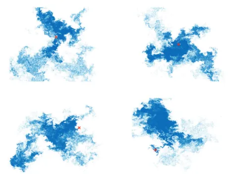
One can have the intuitive picture that on average, an emitted puff of a suspended substance will regularly grow under the effect of diffusion and spread uniformly in space. However, the temporal correlation of the turbulent eddies at all scales bringing together regions of very different concentration values results in creating strong inhomogeneities and gradients. In chapter3, a system of tracer particles continuously emitted from a point source is studied. The additional challenge compared to traditional turbulent mixing lies in the joint effect of spatial as well as temporal correlations in the particles trajectories. The interplay of these correlations is one of the major issues in turbulence. Only in very few models for the carrier fluid these correlations can be analytically treated, like in the Kraichnan ensemble where temporal correlations are fully disregarded (Celani et al., 2007). High resolution direct numerical simulations of inverse turbulent energy cascade are carried, and the issue of measuring the spatial fluctuations of the particle distribution is addressed. To this end, we propose a phenomenological description which allows us to relate the concentration fluctuations along particle trajectories (quasi-Lagrangian mass scaling) with the tracers

(17)

Figure 1.2: Gaussian concentration distribution (colour map) predicted by mean-field ap-proaches do not allow to reproduce fine structures and high concentration levels of trans-ported particles (black dots). The red cross represents the emitting source.

relative dispersion regimes. The idea is to follow an emitted line of particles to quantify its foldings and see how it contributes to the quasi-Lagrangian mass scaling as a function of the distance from the source.

Second part: Modelling particle-laden flows and two-way

coupling

Challenges of inertial particles statistical modelling

This second part starts with chapter 4 which addresses the issue of modelling heavy-particle-laden turbulent flows. The dynamics of such particles is first introduced, and the challenge is stressed to provide a correct modelling of this kind of suspensions, which basically lies in the capacity of the particles to form caustics. The adopted mathematical model must then be able to resolve the velocity dispersion of the particle population. A short review of multiphase models dealing with solid suspensions is also presented.

A novel numerical method is then introduced. Its originality lies in the absence of any form of closing of the kinetic equation associated with the dynamic. This Liouville equation is integrated explicitly in the phase space. Numerical and physical convergence are assessed, and it is shown that the method reproduces with good accuracy the particle distributions obtained via Lagrangian direct simulations.

(18)

9 Turbulent modulation by small heavy particles

Chapter5presents a study about the impact of back-reaction of small heavy particles on a two-dimensional turbulent flow. A short overview of these effects is first presented and the chosen models representing the considered Stokes number asymptotics are introduced. Di-rect numerical simulations of diDi-rect enstrophy cascade are performed, varying the particles mass load. The effect of particles on various statistical properties of the flow is assessed in the asymptotics of low and large Stokes numbers. The modification of global quantities is measured, such as mean energy and enstrophy, as well as the modifications of the scaling in the velocity field through non-linear transfers and dissipations. Impacts on small-scale statistics is also addressed, in particular the modification of intermittency modification. Finally, we also measured how the particles preferential concentration property is affected.

(19)

(20)

CHAPTER

2 Definitions and concepts

Contents

2.1 Navier–Stokes equations . . . 11

2.1.1 Structure functions and intermittency . . . 12

2.2 Turbulence in two dimensions . . . 15

2.2.1 Two dimensional Navier–Stokes equations . . . 15

2.2.2 The double cascade framework . . . 17

2.2.3 Energy and enstrophy budgets . . . 21

2.3 Relative dispersion rates of Lagrangian trajectories. . . 22

2.3.1 Lyapunov exponents . . . 22

2.3.2 Separation rates . . . 23

Concepts and mathematical tools relevant to each chapter will be introduced in their respective opening. As all chapters of this thesis share in common the framework of two-dimensional, incompressible turbulence, the characteristics of such flows are highlighted and compared to their three-dimensional equivalent in this chapter. Some concepts and notations regularly appearing throughout this manuscript are also introduced.

2.1 Navier–Stokes equations

An incompressible velocity field u(x, t) at position x is described by the following equations:

@tu+ (u · r)u = −rp + ⌫r2u+ F , (2.1)

r · u = 0 . (2.2)

(21)

⌫ is the kinematic viscosity, the term ⌫r2 being responsible for the dissipation of large gradients at small scales. p is the pressure which ensures the incompressibility condition (2.2). F denotes the external forcing that maintain the velocity field in a statistically steady, developed turbulent state.

In the absence of dissipation and forcing, i.e. when ⌫ = 0 and F = 0, several quantities, or invariants characterise the flows. In three dimensions, global invariants are energy E = D_kuk2E _{and helicity H = hω · ui. The averaging operation is taken over space and} time in the statistically stationary regime.

Properties of the flow may be assessed through the rate-of-strain tensor, a second order tensor encompassing the gradients of each velocity component u1,2,3, namely:

A = ru = 0 @ @1u1 @2u1 @3v1 @1u2 @2u2 @3v2 @1u3 @2u3 @3v3 1 A.

This matrix, like any, can be decomposed into a symmetric and an antisymmetric part, which are often named Ω and S, respectively:

Ω= 1 2 h ru_{− (ru))}Ti, S= 1 2 h ru+ (ru))Ti. (2.3)

Ωij = 1₂(@iuj − @jui) are the vorticity components, and S = 1₂(@iuj + @jui) the shear

components.

From these tensors, a criterion can be built to determine whether locally in space the flow is dominated by shear or vorticity. In two dimensions, this criterion is given by the Okubo-Weiss criterion W = Ω2− S2 (Okubo, 1970; Weiss, 1991). Due to the Poisson equation for pressure r2_{p = Ω}2_{/2 − S}2_{, the following relation holds for incompressible}

flows: ⌦Ω2↵_{= 2}⌦_S2↵_.

In three dimensions, one can use the Q−R criterion. The matrix A has three invariants under canonical transformations: P = T r(A), Q = −T r(A2_{/2), R = −T r(A}3_{/3). The}

determinant of the characteristic equation for A is then given by ∆ = (27/4)R2_{+ Q}3 _and

the Q − R plan defines 4 regions corresponding to different combinations of eigenvalues of A. Vorticity dominates for large positive ∆ with vortices that are either compressed (R < 0) or stretched (R > 0). On the contrary, strain will dominate for ∆ < 0. See

Cantwell(1993) for more details.

2.1.1 Structure functions and intermittency

The statistics of velocity differences between two points separated by a distance r constitute an important quantity in turbulent flows. Their probability density function gives an important idea about collision probabilities or particles separation rate (see section 2.3). The scaling of their moments also gives information about the scale-invariance of turbulent

(22)

2.1. NAVIER–STOKES EQUATIONS 13 flows. Velocity differences, or increments, are defined by:

δru= hu(x) − u(x + r)i . (2.4)

They constitute a random quantity. When considering homogeneous, isotropic flows, as is the case in this manuscript, δruonly depends on the modulus of r and is independent of

the position x. The structure functions are defined by its moments of various order: Sq(r) =

D

(δk_ru)qE (2.5)

where δrku = δru(r) · r_r is the longitudinal component of δru. Alternatively, one may

also consider S? using the projection of δu(r) on directions orthogonal to r.

The average in (2.5) is taken over the whole space and over time series in the statistically steady regime. In a developed turbulent regime, Sq(r) follows a power-law function of the

scale r:

Sq(r) / r⇣(q) (2.6)

The scaling behaviour is the following. Suppose a large scale forcing at lI of the flow

which is in a statistically stationary state. At scales smaller than lI, statistical quantities

can be assumed to be homogeneous. This is the inertial range. This regimes goes down to a scale ld, the dissipative scale, at which energy is dissipated. In 1941, Andrei

Kol-mogorov made a series of hypothesis that leads to quantitative predictions about velocities increments δru and ld. One is that the energy dissipation rate ✏ > 0 (we choose here to

con-sider this quantity as positive) has a non-zero limit at vanishing viscosity (⌫ ! 0). This is called dissipative anomaly. Another of his hypothesis, shared with Onsager and Heisenberg, sometimes called universality assumption, is that all the small-scale statistical properties are uniquely and universally determined by the scale r and the energy dissipation rate ✏. Given the dimensions of the relevant quantities at play in the inertial range, [δru] = LT−1,

[✏] = L2T−3 and [r] = L, an expression for ✏ follows from dimensional analysis: ✏ ⇠(δru)

3

r . (2.7)

The Reynolds number associated to the scale r reads: Re(r) ⇠ (δr_⌫u)r ⇠ ✏

1/3_r4/3

⌫ , (2.8)

which yields an expression for the dissipative scale corresponding to Re(ld) = 1:

ld= ⌫3/4✏−1/4 (2.9)

Note that it is possible to derive a formal expression for S3. Multiplying the

(23)

S2 as a function of S3, called Karman-Howarth, or simply KH relation. It may then be

solved for S3 in the statistically stationary state (for details of the calculations, seeFrisch

(1995); Landau & Lifshitz (1987)), yielding the only exact result in turbulence known as

the 4/5-law (Kolmogorov, 1941):

S3(r) = −

4

5✏r. (2.10)

This relation implies that there is a constant energy flux in the inertial interval of scales, equal to the one injected at the stirring scale. It also displays that the velocity increments are negatively skewed : particles getting closer are more probable than particles separating. Kolmogorov then assumed strict self-similarity for the velocity differences, i.e. the existence of a unique exponent h such that δk_λru_{⇠ λ}hδkru. This implies that ⇣(q) = hq is

a linear function of q. Requiring (2.10), one gets h = 1/3 hence:

Sq(r) = Cq(✏r)q/3, (2.11)

where the Cp’s are universal dimensionless constants. Furthermore,

The quantity S2 is actually linked to the power-spectra of the velocity. Let us first

define the energy density e(k) in the Fourier space (we note F the Fourier transform), with k the wave-vector: e(k) = 1 (2⇡)d k ˆu_(k)k2 2V = F " X i Rii(r) # . (2.12)

V = Ld _{is the domain volume and R}

ij(r) = hui(x)uj(x + r)i is the velocity correlation

tensor. The following convention for the Fourier transform is used: ˆu(k) =R

Rdeik·r. The kinetic energy spectrum may then be defined in various forms, such as the two following:

E(k) = Z Rd dk0δ(��k0��_{− k)e(k}0) = Z Θk dΩkkd−1k ˆ u_(k)k2 2 , (2.13)

with Θkthe hypersphere in Fourier space of radius k and Ωkthe solid angle element. Owing

to the Parseval theorem, the mean energy in our system can be evaluated either in Fourier or physical space via:

E = 1 V Z Rd ku(x)k2 2 dx = 1 Z 0 E(k) dk. (2.14)

The following relation gives the equivalence between structure functions and spectra. Given a power-law spectrum:

F (k) / k−n, 1 < n < 3, (2.15)

then the second order structure function is also a power-law with (Frisch, 1995): ⌦

(24)

2.2. TURBULENCE IN TWO DIMENSIONS 15 The energy spectrum is sometimes more easily interpretable than the structure function which is its physical pendant. It is also easily obtainable in numerical simulations that use spectral methods to integrate the velocity fields (see appendix A.1).

Using (2.11) and (2.16) for q = 2, one gets

E(k) = ✏2/3k−5/3, (2.17)

which is also the only dimensionally correct combination of ✏ and k. This spectrum shape has been effectively observed in numerical and experimental works. However, in three dimensions, self-similar hypothesis shows to be more and more inexact as the moment q increases (Frisch,1995). Indeed, the exponent ⇣(q) = d log Sq

d log r has been shown to be a strictly

concave function of q, rather than linear. This is called anomalous scaling.

2.2 Turbulence in two dimensions

This thesis work mainly involves two-dimensional turbulent flows, which display some in-teresting features that are phenomenologically different from their three-dimensional pen-dants.

2.2.1 Two dimensional Navier–Stokes equations

In incompressible flows, @iui = 0 so that the two-dimensional velocity field is fully

deter-mined from the function (x, y, t) via the relation u = r?_{= (@}

yux, −@xuy) (the sign of

r?_{may vary in the literature). The level sets of represent the stream-lines, with u being}

everywhere tangent to these level curves, hence the name stream-function for . Vorticity is related to by the relation ! = r ⇥ u = −r2 . The evolution equation for reads:

@t +

1 r2{ , r

2

} = ⌫r2 + f0 (2.18)

where {} denotes the Poisson bracket, or Jacobian, such that {f, g} = @xf @yg − @xf @yg.

Kraichnan (1967) already conjectured that energy would accumulate in the gravest mode

kmin allowed by the boundary conditions (see below section2.2.2). This accumulation of

energy at large scale would eventually a condensate (illustrated in Figure 2.1), analogous to a Bose-Einstein condensate.

In the real world, mechanisms arise from various physical origins to prevent this large scale energy piling up, like Rayleigh friction in stratified fluids or the friction induced by the surrounding air in soap-film experiment. An additional linear term −↵ is often added in Navier-Stokes equations to represent this friction, so that f0 = f _{− ↵ . ↵ is} thus the Ekman friction coefficient responsible for the large scale energy dissipation. It is often used in numerical simulations to reach a statistically stationary state, especially in the two-dimensional inverse cascade (Salmon, 1998). The origin of its linear form may

(25)

Figure 2.1: Vorticity condensate in the two dimensional inverse cascade. FromBoffetta &

Ecke(2012).

be exemplified the following way: near solid boundaries with no-slip condition, a laminar Poiseuille profile is usually admitted. Say the surface is horizontal at z = h, with z the vertical direction, then the velocity reads u(z) = _2⌫↵_{(z − h)}2 and ⌫(@_x2+ @_y2+ @_z2_)r2u _⇠ ⌫(@2

x+@2y)u−↵u. In experiments, it is also this drag form that is adopted for liquid friction

on a soap film, or with the bottom of a container. Also ion-neutral collisions in ionospheric plasma give rise to such a friction.

The equivalent equation for the vorticity is obtained by taking minus the Laplacian of equation (2.18):

@t! + u · r! = ⌫r2! − ↵! + f! (2.19)

! is written in non-bold font to explicit that it is treated as a scalar quantity in the 2D plane: the vortex lines are always perpendicular to the flow plane. Equation 2.19, except for the forcing f!, expresses vorticity transport by the flow and dissipation by small-scale molecular

viscosity and large-scale friction. One important difference between (2.19) compared to its 3D equivalent is the lack of the vorticity stretching term (ω · r)u which is identically 0 in 2D. In 3D, it is responsible for vorticity amplification in the vortex stretching direction due to angular momentum conservation.

(26)

2.2. TURBULENCE IN TWO DIMENSIONS 17

2.2.2 The double cascade framework

Global invariants

Neglecting the large-scale friction and force terms in (2.19) and multiplying (2.19) by ! and averaging, one gets DtZ = ⌫r2! where

Z = 1 2 ⌦

!2↵ (2.20)

is the enstrophy. Thus, for inviscid flows (⌫ = 0), enstrophy is conserved along Lagrangian trajectories1_{. Actually,}R _!n_d2_x_{is a constant of motion for all n > 0. In two-dimensional}

turbulence, enstrophy and energy are the quadratic invariants.

To give an intuition about the mechanism at play, the unforced Navier–Stokes equations for the velocity Fourier coefficients are first introduced:

@tuî(k) + ✓ δij− kikj k2 ◆ X k=p+q ipjuî(p)ûj(q) = −⌫ kkk2uî(k). (2.21)

The second term on the left-hand side is the Fourier transform of the non-linear term. It shows that the mode k interacts with modes p and q such that p = q + k, i.e. p, q and k must form a triangle. This is called a triadic interaction, and conserves both energy and enstrophy.

In order to grasp the essence of energy transfers in two-dimensional turbulence, one can refer to the paper by Kraichnan (1967) who deduced the direction of the cascades of energy and enstrophy with statistical mechanics arguments. The term cascade refers to the fact that the injected energy (or enstrophy) is transferred at a constant rate through the scales. This transfer results from the non-linear term in (2.1) and takes place until molecular dissipation counter-balances at the dissipation scale.

Another phenomenological argument was already advanced byFjørtoft(1953) to predict the direction (in the scale space) of these transfers. A triadic interaction between wave-numbers k1< k2< k3conserving both energy and enstrophy, we have that their variations

must vanish: P_i∆_E_i₌P iki2∆Ei= 0. Therefore: ∆_E₁₌ k 2 2− k32 k2 3− k12 ∆_E₂ ∆_E₃₌ k 2 1− k22 k2 3− k12 ∆_E₂_. _(2.22)

This implies that when mode k2 loses energy (∆E2< 0), more energy will go into k1 than

k3, indicating a direction of energy toward large scales. Similarly, more enstrophy must go

into k3 than k1, so that enstrophy is transferred to small scales.

It also implies that the energy and enstrophy transfers must take place in two different directions in the |k| space.

1_{In three dimensions, an additional term appearing in the vorticity equation, called vortex stretching,}

(27)

The direct enstrophy cascade is considered to be the process responsible for vorticity filaments stretching and folding, creating stronger and stronger vorticity gradients until they are eventually dissipated by molecular viscosity. See (Kraichnan & Montgomery,

1980; Monin & Ozmidov, 1985) for details.

Spectrum scaling in the dual cascade

The energy and enstrophy spectra are related through Z(k) = k2E(k). In the inverse cas-cade, under the assumption of Kolmogorov phenomenology, the energy spectrum exponent is identical to the one in three dimensions:

E(k) = C1✏2/3k−5/3, (2.23)

Z(k) = C1✏2/3k−1/3, (2.24)

where ✏ is the energy dissipation rate and C1 is a constant, determined to be in the range

⇠ 5.8 − 7.0 (Paret & Tabeling, 1997).

In the direct enstrophy cascade, the spectra are:

E(k) = C2✏2/3! k−3[ln(k/kf)]−1/3, (2.25)

Z(k) = C2✏2/3! k−1[ln(k/kf)]−1/3. (2.26)

where ✏! represents this time the enstrophy dissipation rate, analogous to ✏ for energy.

kf = 2⇡/lf denotes the forcing wave-number corresponding to the forcing length lf.

The presence of the logarithmic factor in (2.25) and (2.26) is a correction that ensures that the enstrophy flux is constant across the inertial range (seeKraichnan(1971);Rose &

Sulem(1978) for details), This factor is important for regularity reasons. Indeed, the total

enstrophy Z =R k2_{E(k)dk ⇠ kr · uk}2 _{with E(k) / k}−3 logarithmically diverges, and the velocity field is not differentiable. It also implies that enstrophy fluxes are less local (i.e., contributions to the flux at k can come from a much wider range of wave-numbers around k) than their energy pendants.

Those scalings for energy and enstrophy spectra have been indeed observed in numerical studies, already inBorue(1994), and experimentally in large-scale geophysical or quasi-2D stratified flows and soap films (Boer et al., 1984; Rivera & Wu, 2000; Daniel & Rutgers,

2002). Figure 2.2, coming from a direct numerical simulation at very high resolution

(Boffetta & Musacchio, 2010), illustrates these two regimes.

In the inverse cascade, one can also derive an expression for S3(r) in the same way than

in three dimensions (see section2.1). It reads: S3(r) =

4

3✏r. (2.27)

Compared to (2.10), S3 is positively skewed in two dimensions. In the direct cascade, the

(28)

2.2. TURBULENCE IN TWO DIMENSIONS 19 10-10 10-8 10-6 10-4 10-2 100 1 101 102 103 104 E(k)/ εα 2/3 k A B C D E 0.1 1 10-6 10-5 δ ν

Figure 2.2: Energy spectra of two dimensional flows, obtained via Direct Numerical Sim-ulations for spatial resolution up to 327682 (from Boffetta & Musacchio(2010)). In those simulations, the forcing wave-number is set at kf = 100.

Effect of Ekman friction

Due to the energy flow toward the large scales in the two dimensional inverse cascade, it is necessary to provide a low-k energy sink if ones wants to achieve statistical stationary state. This is why the Ekman friction term is so important in two-dimensional simulations. This term however has some impact on the flow structure. For example, it was shown

byNam et al.(2000);Bernard(2000);Boffetta et al.(2002) in the direct enstrophy cascade

that as the friction coefficient ↵ increases, so does the enstrophy spectrum slope, deviating more and more from the Kraichnan prediction, i.e. E(k) / k−(3+⇠)where ⇠ is related to the distribution of finite time Lyapunov exponents (see below). A consequence of (2.15) and (2.16) is that for ↵ = 0, ⇠ = 0 and for 0 < ⇠ < 2, ⇠ = ⇣!

2, where ⇣! is the vorticity structure

function exponent. The slope steeper than k−3 _{when ↵ > 0 implies the differentiability of}

the velocity field (see section 2.2.2) and the logarithmic correction in (2.25) and (2.26) is absent.

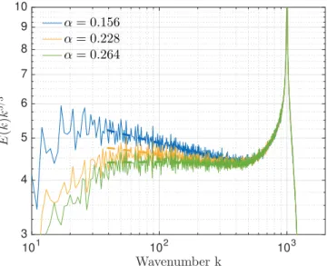
In the inverse energy cascade range, it may be shown that the effect is the reverse: as ↵ decreases, energy builds up into a large scale condensate. The apparent effect is a steepening of its slope. This tendency is illustrated for various spectra coming from the simulations with resolution N2

x = 40962 performed in the framework of the study at

chapter 3. The value of ↵ was selected in such a way that the accumulation of energy is prevented at large scales, without depleting too much the inertial range cascade in order

(29)

101 102 103 Wavenumber k 3 4 5 6 7 8 9 10 E (k )k 5/ 3 α= 0.156 α= 0.228 α= 0.264

Figure 2.3: Energy spectra for various Ekman friction coefficients ↵ in the two dimensional inverse energy cascade with kf = 103. The spectra are compensated by kkk5/3.

Dashed-lines represent fit in the inertial-range. Contrary to the direct cascade, the slope diminishes as the friction coefficient increases.

to get a spectral slope as close as possible to k−5/3_.

Intermittency in 2D turbulence

While the velocity field in three dimensions is known to be intermittent, the direct and inverse cascade deserve separate discussion in the two-dimensional case. In the inverse energy cascade, dimensional scaling was observed in numerical simulations by Boffetta

et al. (2000) for the Lagrangian structure function of order up to p = 7, ruling out the

possibility of intermittency similar to that in the 3D case. They nevertheless observed an antisymmetric part for high fluctuations of the longitudinal velocity differences, so that there is no Gaussianity. Other experimental and numerical works lead to the same conclusion (Paret & Tabeling, 1998; Chen et al., 2006b;Xiao et al.,2009).

In the direct cascade, velocity doesn’t display any intermittency, so that its incre-ment are Gaussian even at small scales. Rather, it is the vorticity structure function that displays anomalous scaling. The exponents ⇣(p) of Sp may be related to the following

dynamical argument. As stated in section 2.1, the Lyapunov exponent λ is obtained in the limit when two initially close trajectories in chaotic flows have diverged during an in-finite time. When this time t is in-finite, these exponents depend on initial separations and are characterised, owing to the large deviation principle, by a probability density

(30)

func-2.2. TURBULENCE IN TWO DIMENSIONS 21 tion P (λ|t) =ptG00_{(λ)/2⇡ e}−tG(λ) ₍_Ott_,₂₀₀₂_{). The convex Kramer function G(λ) is then}

related to the exponents by the relation ⇣2n = min

h [2q, (G(λ) + 2q↵)/λ] (Neufeld et al., 2000). This implies that the probability density function of the vorticity increment is not self-similar and deviates from Gaussian at small scales (Tsang et al., 2005).

A third sign of intermittency is the multifractal property of the vorticity dissipation field, kr!(x)k2. One way to get a measure of a chaotic attractor in a give phase space is to look at its Renyi dimension spectrum Dq. Dividing the phase space in (hyper)-cubes Cj

of size ✏, Dq is defined by (Renyi, 1970):

Dq = lim ✏!0 1 1 − q log⇣P_jµ(Cj)q ⌘ ln(1/✏) . (2.28)

µ is the natural measure associated with the attractor such thatP_jµ(Cj) = 1. Dq is a

non-increasing function of q and is independent of q for non-fractal attractors. In particular, D1 is the information dimension and D2 the correlation dimension. These dimensions

may be determined numerically using box-counting algorithms (see section 3.3.2 for an example of the measure of D2). Tsang et al. (2005) showed that anomalous scaling of

the vorticity structure function yields multifractality of vorticity dissipation through the relation Dq = 2 +⇣2q_q−1−q⇣2.

2.2.3 Energy and enstrophy budgets

One can derive the equations for the evolution of the fluid energy and enstrophy by mul-tiplying Navier-Stokes equations (2.18) respectively by the fluid velocity u and vorticity !. Only the energy conservation terms are written, the case of enstrophy being analogous. The equation for the instantaneous variations of the shell-averaged energy content at wave numbers such that kkk = k reads:

@tE(k) + Π(k) = −2⌫Z(k) + −↵E(k) + F (k). (2.29)

Π(k) = hu · (u · ru)i is the non-linear transfer contribution which satisfies

Z 1

0

Π(k) dk = 0. (2.30)

This term also corresponds to the integral of the triadic interactions over the wave-numbers kkk = k. This quantity, represented along the k axis, allows one to better visualise the cascades. Indeed, representing Π<(k) = R₀kΠ(k) dk on a plot with a logarithmic scale in the wavenumber dimension displays a plateau, i.e. a constant flux.

For example, in the inverse energy cascade, the energy goes from low to large values of k. Π<_{(k) is thus a source term for the large scales (larger than the forcing scale). Hence,}

(31)

10

0

10

2

Wavenumber k

-0.02

-0.01

0

0.01

0.02 Π(k)

−

α

E(k)

−2

ν

E(k)

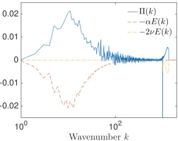
Figure 2.4: Illustration of the terms appearing in the spectral energy budget (2.29) in the inverse cascade at a resolution N2

x = 40962. The peak in the non-linear transfer is due to

the stochastic forcing injected at the corresponding scale.

plateau. In the direct cascade, this term would be constant and positive for the enstrophy budget, as this quantity cascades to the small scales.

The energy dissipation has two contributions, which are on average negative for all k. One comes from molecular viscosity with total dissipation ✏ = R₀12⌫Z(k) dk, the other one from Ekman friction with total dissipation ✏↵ =

R1

0 ↵E(k) dk. The term F (k) =

h ˆu_{(k) · f(k)i denotes the input power at scales k, where the average is taken over} wave-numbers with modulus k.

Figure 2.4 illustrates the non-linear term along with the friction term appearing in equation (2.29). Those simple relations may serve as a benchmark when designing Navier-Stokes solvers. In a statistically steady state, h@tE(k)i is zero, and the other terms must,

on average, balance.

2.3 Relative dispersion rates of Lagrangian trajectories

2.3.1 Lyapunov exponents

One important quantity to characterise the dynamics of transported elements in chaotic flows, coming back from the works of Lyapunoff (1907), describes how two tracers in-finitesimally close do separate asymptotically in time following the continuous stretching, contractions and rotations of their separation vector. Tracers are particles that follow ex-actly fluid stream lines and can be thought as attached to fluid elements, hence their name

(32)

2.3. RELATIVE DISPERSION RATES OF LAGRANGIAN TRAJECTORIES 23 (see3.1.1). They are characterised by their position X, and velocity V = u(X), which is the fluid velocity at their position. Their equation of motion reads:

˙

X= u(X, t). (2.31)

Considering the tangent bundle in the phase-space R(t) = δX(t) at point X(t), its evolution reads:

dR(t)

dt = σ(t)R(t), (2.32)

with σij = @jui(X(t)) denoting the Lagrangian strain matrix. The integral

J = exp₀ ✓Z t 0 σ(s)ds ◆ , (2.33)

with exp_o the time-ordered exponential, is the Jacobian matrix such that R(t) = JR(0). Consider an initial volume of fluid which is evolved by the dynamic. It will be elongated along some directions and stretched along others. Actually, for each single trajectory and in the limit t ! 1, the orientation of this ellipsoid’s axis will have converged (due to the Multiplicative Ergodic Theorem by Oseledec (Oseledec, 1968)) in the directions of the eigenvectors ej of the matrix JTJ. Indeed, with R(t) = J R0 then kRk2 = RTR =

R0JTJ R0. JTJ is a symmetric matrix, hence diagonalisable. Because it is also positive,

its eigenvalues are positive and may written in the form of an exponential eλjt_{, defining} the Lyapunov exponents:

λj= lim t!1

1

tln (|Jej|) j = 1, . . . , 2d. (2.34)

The evolution rate of a phase-space volume is given by ✓ =P2d_j=1λj. In incompressible

flows, this sum is zero, and the volumes are thus conserved. To provide another example, as will be discussed in 4, for inertial particles, whose dynamic is dissipative, this sum is negative, yielding a contraction rate with a given characteristic time which is a property of the particles.

These Lyapunov exponents may be used to define a fractal dimension of a phase-space attractor, called the Lyapunov dimension. Ordering the exponents in decreasing order and defining the partial sum S(i) = Pi_jλj, then dL is the interpolated index for which

S(dL) = 0. The Kaplan–Yorke conjecture (Kaplan & Yorke, 1979; Eckmann & Ruelle, 1985) then states that the information dimension of the attractor D1 is equal to dL.

2.3.2 Separation rates

The velocity of the relative separation between two tracers is not a trivial quantity in turbulence.

Denoting by R(t) = Xi_{(t) − X}j_{(t) the separation between two particles i and j at time}

(33)

may depend on multiple factors like the initial and present separations R(0), R(t) and the statistics of the fluid velocity differences projected on their separation vector

δRu = (ku(x)k − ku(x + R)k) ·

R

kRk. (2.35)

Smooth flows

Consider first two particles separated by a distance below the dissipation scale ld, i.e. in

the dissipative range. The flow is then differentiable and Lipschitz in R, i.e. δRu⇠ σR,

ensuring the unicity of the solution of (2.31). The particles then separate exponentially in time with the Lyapunov exponent λ:

kR(t)k = kR0k eλt. (2.36)

Non-smooth flows

Consider now two particles initially separated by kR0k which is in the inertial sub-range.

In this range, in the 3D direct cascade or 2D inverse cascade, velocity field is no longer smooth: hδrui / r1/3. This implies dR2/dt = 2R · δRu/ R4/3 and:

D

kR(t)k2E

R0 / g

Rt3, (2.37)

where gR is the Richardson constant and the average is taken over particle pairs initially

at distance R0. This rate is faster than diffusion (R2(t) / t) and the regime is called

super-diffusive, faster than what can be attributed to sole chaotic motions. Indeed, in the exponential separation (see paragraph above), the time for two particles to reach a scale R diverges logarithmically with R/R0. On the contrary, the explosive separation does not

depend on the initial separation R0 and particles will always reach R in a finite time.

This observation was already predicted by Richardson (1926). He measured a scale-dependant diffusivity K which fits well with K(r) / r4/3 _{on 4 decades. Indeed, a}

contam-inant cloud of size r is only advected by vortices larger than r, and its diffusions results mainly from vortices of size r. From this result, he derived equation (2.37) using Fickian dif-fusion. This scaling law for K(r) was later formulated in the framework of the Kolmogorov theory following the Obukhov hypothesis (Obukhov,1941). If r is in the inertial range, the effective diffusivity K(r) must only depend on r and ✏, leading to K(r) / ✏1/3r4/3.

This super-diffusive behaviour however was showed by (Batchelor,1950) to be preceded by a ballistic separation, i.e. with a velocity constant in time, for which we getD_kR(t)k2E= C(✏R0)2/3t2. This regime is valid during the correlation time of the eddies of size R0. This

correlation time is typically of the order of the eddy turn-over time associated with the scale R, ⌧R / ✏−1/3R2/3. From this observation, Bourgoin (2015) and Thalabard et al.

(34)

2.3. RELATIVE DISPERSION RATES OF LAGRANGIAN TRAJECTORIES 25 (2014) successfully proposed to interpret the explosive separation as an iterative ballistic process.

This Richardson dispersion regime is also associated with another issue about the re-versibility of pair separations: in three dimensions, the Richardson constant gR is not the

same when considering the forward in time evolution of pairs and its backward in time equivalent. Heuristically, this can be understood by the fact that the odd number of di-mension allows a fluid ellipsoid to be elongated along more didi-mensions than those along which it can be squeezed. This would not be the case in two dimensions.

(35)

(36)

Part I

Turbulent dispersion and mixing

(37)

(38)

CHAPTER

3 Tracers dispersion in two dimensional turbulence

Contents

3.1 Introduction . . . 29

3.1.1 Diffusion at long times . . . 33

3.1.2 Continuous source . . . 36

3.2 middling version . . . 36

3.2.1 Fluid phase integration . . . 36

3.2.2 Injection mechanism . . . 38

3.2.3 Removal mechanism . . . 39

3.3 Results. . . 39

3.3.1 One point dispersion . . . 39

3.3.2 Two-point correlation . . . 43

3.3.3 Phenomenological description . . . 49

3.4 Brief conclusion . . . 54

3.1 Introduction

Turbulent mixing is of particular concern in situations such as the formation of clouds through condensation of small water droplets (Grabowski & Wang,2013), gas accretion in planet formation (Johansen et al.,2007) or phytoplankton and nutrients distribution in the oceans (Mann & Lazier, 2013). Mixing refers to the evolution of an initial distribution of a scalar field (temperature, salinity, or the concentration of any substance...) by the fluid.

(39)

The mechanical stress induced by the stirred flow tends to deform the initial distribution of this field, and the multi-scale nature of turbulent flows gives rise to very complex shapes and patterns of the concentration field (Celani et al.,2001). For example, while the scalar is also submitted to molecular diffusion, which tends to smooth out concentration gradi-ents, mixing by stretching and compression in directions orthogonal to each other cause to reinforce these gradients by creating elongated concentration filaments.

Because incompressible flows preserve volumes, an homogeneous initial scalar tration remains uniform at any later time. However, non-uniform initial patches of concen-trations will be deformed by the swirling eddies and create locally high gradients. Figure3.1 displays an instantaneous field of scalar concentration advected by a turbulent flow: large fronts and cliffs are seen along with rather uniform regions. These gradients form because turbulence brings close together trajectories of fluid elements carrying different scalar tra-jectories and history. Scalar differences over small scales grow in intensity while the front boundaries become thinner, until they are eventually dissipated by molecular viscosity. These large differences are responsible for strongly intermittent statistics in the scalar dis-tribution (Sreenivasan & Antonia, 1997), i.e. the probability density function (pdf) of scalar value shows a departure from a Gaussian behaviour, and displays exponential tails

(Pumir et al., 1991) that result from rare, extreme events. They prove that a restrictive

vision considering a large number of small-scales, uncorrelated stretching events for the scalar distribution, which would yield Gaussian pdf through the central-limit theorem, is not correct.

Interestingly, the passive scalar is strongly intermittent both in 2D and 3D even in the absence of intermittency in the velocity field itself in 2D, and also in simple random Gaussian velocity fields (Shraiman & Siggia,2000). Similarly to the velocity increments in 3D or the vorticity in the 2D direct cascade, the scaling exponents of the scalar structure function S_✓n_{(r) = h(✓(x) − ✓(x + r))}n_{i / r}⇣(n) _{are not linear: ⇣(n) 6= n/3 (see section} 2.1.1). Scale invariance is thus broken and Sn reads (Celani & Vergassola,2001):

S_✓n_{(r) / r}⇣dim(n)✓ L r

◆⇣dim_(n)−⇣(n)

(3.1) The difference ⇣dim_{(n) − ⇣(n) is the correction for the anomalous scaling, and the broken}

scale invariance manifests in the presence of L although r ⌧ L.

Some analytical models for the velocity correlations, like the Kraichnan model ( Kraich-nan,1994), allow to recover predictions about the behaviour of limn!1⇣(n). In the

Kraich-nan ensemble, the two-points, two-times velocity correlation are:

hvi(x1, t2)vj(x2, t2)i = Dij(xi− xj)δ(t1− t2) (3.2)

with

Dij(r) = D0δij− D1r⇠[(d + ⇠ − 1)δij− ⇠

rirj

(40)

3.1. INTRODUCTION 31 for r smaller than the integral scale. ⇠ denotes the degree of roughness of the flow: the velocity field smoothness increases with ⇠ and is differentiable for ⇠ = 2.

In this model, and under the additional assumption of high dimensionality, d � ⇣(2), it was analytically shown in Balkovsky & Lebedev(1998) that there exists a critical order nc such that 8n > nc, ⇣(n) is independent of n This asymptotic behaviour seems also to

be observed with direct numerical simulations of two dimensional inverse cascade, where it was estimated in Celani et al.(2000).

As vorticity and passive scalar share the same transport equation, it is tempting to com-pare their scaling laws to see if the exhibit similarities. However, the direct link between ! and u make the equation for ! non-linear, which can lead to discrepancies for small scale quantities. For example,Dubos & Babiano(2003) have shown using numerical simulations that this difference is responsible for faster temporal fluctuations of the vorticity gradients.

In Boffetta et al.(2002), a correspondence is made between the intermittency of vorticity

and that of a passive scalar transported by the flow, showing that ⇣_p! = ⇣_p✓_{8p. This} corre-spondence may be explained using the following ad-hoc argument (Tsang et al.,2005) based on the Lyapunov exponent λ (see section 2.3_{). Since λ ⇠}D_kruk2E1/2_⇠qR_k1

f k

2_{E(k) dk}

and assuming, then λ ⇠ k−⇠/2f . Thus λ (and ru) characterising small separations

stretch-ing, are determined by large scale structures, and the small scale vorticity components behave like scalar advected by the large scale flow.

Structure functions of order n are linked to the equal time n-point correlation function of the scalar field. For example, consider the following equality for n = 2:

S2(r, t) =

D

(✓(x + r, t) − ✓(x, t))2E (3.4)

=⌦✓(x)2↵+⌦✓(x + r)2↵_{− 2 h✓(x + r, t)✓(x, t)i} (3.5)

= 2 (C2(0, t) − C2(r, t)) . (3.6)

The last equality results from homogeneity and isotropy and C2(r, t) = h✓(x + r, t)✓(x, t)i.

Averages are taken over the positions x.

The generalisation of this quantity to n-points displays the link with the n-point joint transition probability for the Lagrangian motion. For a set of n particles initially at position x0, . . . , xn at instant t0: Cn(x1, . . . , xn; t) = h✓(x1, t), . . . , ✓(x2, t)i (3.7) = t Z t0 ✓(x0₁, t), . . . , ✓(x0₂, t0) pn(x1, . . . , xn, t|x01, . . . , x0n, t0) dx01. . . dx0n (3.8) where p(. . . ) expresses the joint probability that the n trajectories initially at positions x0₁. . . , x0

(41)

The quantity Cn can be related to the joint motion of n particles. It has a geometrical

interpretation in terms of Lagrangian trajectories. For example, in Celani & Vergassola

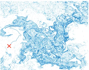
(2001), the intermittency of the passive scalar advection is attributed to long lasting clus-tering of n-tuple of particles. In Bianchi et al. (2016), the shape of spherical puffs of particles emitted is monitored as a function of time, showing that although the puff is initially spherical, the quick and strong distortions prevent the cloud to return back to a spherical shape at later times. It is also shown not to affect much large scale transport statistics, like the pdf of durations of hits and between hits of a downstream target.

In particular, the two-point scalar correlation allows one to express pair dispersion statistics. This correspondence was for example used in Boffetta & Celani(2000) to link frequent pairs encounter and scalar fronts formation. This object, C2(r) may be analytically

derived only under drastic constrain on the flow, like for example the Kraichnan ensemble, In such a flow, Celani et al.(2007) have studied scaling properties of a scalar continuously emitted from a point source and derived an exact relation for the two-points equal-time scalar correlation function C(x1, x2, t) = h✓(x1, t)✓(x2, t)i, demonstrating the persistence

of inhomogeneities at small scales.

Figure 3.1: Illustration of a scalar field mixed by turbulent flow, representing a 2D slice from a 3D DNS simulation at N_x3= 40963with a mean gradient scalar source. When initial inhomogeneities or inhomogeneous scalar sources are present, mixing by eddies create fronts where the scalar variations over very small scales are of the same order than the rms value itself.