HAL Id: hal-01108898
https://hal-paris1.archives-ouvertes.fr/hal-01108898
Submitted on 23 Jan 2015
HAL is a multi-disciplinary open access
archive for the deposit and dissemination of
sci-entific research documents, whether they are
pub-lished or not. The documents may come from
teaching and research institutions in France or
abroad, or from public or private research centers.
L’archive ouverte pluridisciplinaire HAL, est
destinée au dépôt et à la diffusion de documents
scientifiques de niveau recherche, publiés ou non,
émanant des établissements d’enseignement et de
recherche français ou étrangers, des laboratoires
publics ou privés.
Feature Relations Graphs: A Visualisation Paradigm for
Feature Constraints in Software Product Lines
Jabier Martinez, Tewfik Ziadi, Raul Mazo, Tegawendé F. Bissyandé, Jacques
Klein, Yves Le Traon
To cite this version:
Jabier Martinez, Tewfik Ziadi, Raul Mazo, Tegawendé F. Bissyandé, Jacques Klein, et al.. Feature
Relations Graphs: A Visualisation Paradigm for Feature Constraints in Software Product Lines. IEEE
Working Conference on Software Visualization (VISSOFT 2014), Sep 2014, Victoria, Canada. pp.50
- 59, �10.1109/VISSOFT.2014.18�. �hal-01108898�
Feature Relations Graphs: A Visualisation Paradigm
for Feature Constraints in Software Product Lines
Jabier Martinez
1,2, Tewfik Ziadi
2, Raul Mazo
3, Tegawend´e F. Bissyand´e
1, Jacques Klein
1and Yves Le Traon
11SnT, University of Luxembourg, Luxembourg 2LiP6, University Pierre et Marie Curie, France 3CRI, Panth´eon Sorbonne University, France
[email protected], [email protected], [email protected] {tegawende.bissyande, jacques.klein, yves.letraon}@uni.lu
Abstract—Software Product Line Engineering is a mature approach enabling the derivation of product variants by assem-bling reusable assets. In this context, domain experts widely use Feature Models as the most accepted formalism for capturing commonality and variability in terms of features. Feature Models also describe the constraints in feature combinations. In industrial settings, domain experts often deal with Software Product Lines with high numbers of features and constraints. Furthermore, the set of features are often regrouped in different subsets that are overseen by different stakeholders in the process. Consequently, the management of the complexity of large Feature Models becomes challenging. In this paper we propose a dedicated interactive visualisation paradigm to help domain experts and stakeholders to manage the challenges in maintaining the con-straints among features. We build Feature Relations Graphs (FRoGs) by mining existing product configurations. For each feature, we are able to display a FRoG which shows the impact, in terms of constraints, of the considered feature on all the other features. The objective is to help domain experts to 1) obtain a better understanding of feature constraints, 2) potentially refine the existing feature model by uncovering and formalizing missing constraints and 3) serve as a recommendation system, during the configuration of a new product, based on the tendencies found in existing configurations. The paper illustrates the visualisation paradigm with the industrial case study of Renault’s Electric Parking System Software Product Line.
I. INTRODUCTION
Modern software development often leads to software prod-uct variants that share a set of commonalities and differ in a few variability points. There is thus today a momentum for Software Product Line Engineering (SPLE) [24] as a suitable paradigm of software development for reducing both the maintenance effort and the time to market. In this context, practitioners and researchers alike, rely on Feature Models (FMs) [16], [25] as the main formalism for capturing com-monality and variability of products in terms of features. A feature is defined as a prominent or distinctive and apparent aspect, quality, or characteristic of a system [16]. A given FM describes the set of valid combinations of features, referred to as configurations, for the system. Visually, the FM is often represented in a diagram, as illustrated by Figure 1 regarding a Car FM. The hierarchy of features includes mandatory features (Gear, Car), optional features (DriveByWire, ForNorthAmer-ica), alternative features (Manual or Automatic), and other po-tential constraints such as feature implications (DriveByWire
requires Automatic). Implications and mutual exclusions are referred to as hard constraints since no valid configuration can violate these constraints. However, there exists other constraints, known in the literature as soft constraints [9], whose violations do not lead to incorrect configurations. Such constraints are used during the configuration process of a new product to provide suggestions in feature selections. In the Car example, based on domain expert knowledge, selecting the ForNorthAmerica feature could suggest the selection of Automatic gear.
Real-world SPLs yield FMs that can be large and complex with thousands of features and as many constraints. As an example, researchers have already reported the challenges of dealing with the 8000 features of the Linux kernel [28]. In general, FM constraints are initially formalized by the different stakeholders at the domain engineering step. However, the evo-lution of the SPL could require modifying or adding features and new hard and soft constraints could appear requiring a refinement of the existing FM. Such large FMs present many issues for human comprehension. Apart from that, with such numbers of features and constraints it is possible to have non formalized constraints. Non formalized constraints are those that exist implicitly but that are not explicitly defined in the FM. Consequently, non formalized constraints could be the cause of potential invalid derived products. Extracting algorithmically the constraints of the FM can be useful to formally analyse the SPL and ensure that it is consistent with actual (i.e., already instantiated) and future configurations. Mining non formalized FM constraints from existing configu-rations is known however to be a challenging endeavour in the community of SPLE. A large body of literature is dedicated
Fig. 1: Example of Car Feature Model. Credits to Czarnecki et al. [9]
to this issue. Most approaches [12], [15], [18], [19], [26], [31] target hard constraints, while others also propose algorithms to extract soft constraints [9]. Once constraints are mined, they must be confirmed by the different stakeholders. Unfortu-nately, from the domain expert perspective, enumerating and displaying hundreds of constraints will inevitably lead to a tedious investigation analysis. A promising alternative would be to provide a visualisation paradigm that is more intuitive than a textual listing, and also provides free exploration.
Visualization and interactive techniques are widely accepted to reduce the complexity of comprehension tasks [6]. We contribute in this paper with a new visualization paradigm for feature constraints, i.e., relations. We present our approach for building Feature Relations Graphs (FRoGs), and we present experimental results in an industrial case study.
A FRoG representation targets different stakeholders (e.g., domain experts, product developers, and users) and different usage scenarios (design analysis, documentation, and recom-mendation).
The main contributions of this paper are:
• We propose a new visualization paradigm to intuitively represent the relations among features in an SPL. • We propose an approach for mining constraints from
existing configurations to feed our visualization tool. • We demonstrate the usability of our tool in different usage
scenarios, based on a real-world dataset from a major manufacturer.
The remainder of this paper is structured as follows: Section II presents the background of managing constraints in SPLE to motivate our work. Section III formalizes the data abstractions and describes our proposed visualization paradigm. Section IV presents the case study. In Section V we discuss related work and Section VI concludes and presents future work.
II. BACKGROUND ANDMOTIVATIONS
In practice, as discussed in the literature [16], [25], a FM may contain hard constraints that express strong dependencies between features. Following the Car example, we cannot have the DriveByWire feature without the Automatic gear feature. The explicit formalization of such constraints assures the assembling of valid feature combinations that will violate neither structural nor semantic dependencies of the product variant that has to be created. Therefore a given FM describes the set of valid combinations of features. Each combination, referred to as configuration corresponds to a specific product. Table I shows all the possible valid configurations of the Car example. Although Gear and Car, as shown in Figure 1, are also features of the Car example FM, they are not in Table I because they are mandatory features that do not represent variation points for the SPL.
FMs could be expressed as propositional formulas as pre-sented in [1], [10]. The “inclusion” implication constraints are expressed with the requires statement and “exclusion” constructions are expressed with the excludes statement:
• requires: Example: A ⇒ B. Feature A requires the presence of feature B.
• excludes: Example: A ⇒ ¬B. Feature A excludes the presence of feature B.
In the illustrative FM of Figure 1, a mutual exclusion (Automatic ⇒ ¬M anual, M anual ⇒ ¬Automatic) is formalized through the Alternative construction. However, a domain expert can also add hard constraints explicitly between any features in the FM hierarchy as for example DriveByW ire ⇒ Automatic. Notice also that, because of logic inference rules, we can have hard constraints that are not explicitly formalized but that exist because of the other formalized constraints. This relation type between features is called inferred constraint. For example DriveByW ire ⇒ ¬M anual is an inferred constraint.
The presence of two features in a given product configura-tion can also be qualified in terms of suitability. Such relaconfigura-tions between features have also been explored in the literature. B¨uhne et al. [5] refer to them as hints and hinders relations. In the Pure::Variants commercial tool [3], the terms encourage and discourage are used in reference to the constraints in such relations. Czarnecki et al. [9] formally refer to them as two particular types of soft constraints, in the sense that their violation does not give raise to incorrect configurations. They exist with the objective of alerting the user, providing suggestions during the configuration process [9] or as a way to capture domain knowledge related to these trends. We will use the notation below for soft constraints:
• encourages: Example: sof t(A ⇒ B). Feature A encour-ages the presence of feature B.
• discourages: Example: sof t(A ⇒ ¬B). Feature A dis-courages the presence of feature B.
This way, a domain expert of the Car example could explic-itly formalize the soft constraint sof t(F orN orthAmerica ⇒ Automatic) mentioned before to capture this SPL domain knowledge.
In addition to features, constraints and configurations, the FM has the particularity to be addressed by different stake-holders at the same time. Indeed, and as mentioned by Yu et al. [32], variability in FMs arises from different stakeholders goals. Each stakeholder can thus be interested in a partial view of the variability included in a FM. In other words, each stakeholder has its own stakeholder perspective. For instance, features concerning the type of Gear in the Car example is mainly useful for final customers to choose their cars. However, DriveByWire is more the concern of engineers
TABLE I: Valid Configurations for the Car example.
Manual Automatic DriveByWire ForNorthAmerica f1 f2 f3 f4 Conf 1 X X Conf 2 X Conf 3 X Conf 4 X X Conf 5 X X X Conf 6 X X
during the construction of the cars, while the ForNorthAmerica feature can be related to commercials and sales analysts. Each stakeholder perspective cannot ignore the impact of other features from other stakeholders perspectives. Consequently, fluent communication means should exist to reason about these feature relations that involves different stakeholders, called inter-stakeholder perspectives constraints hereafter.
As reported by [21], “the use of visualisation techniques in Software Product Line can radically help stakeholders in supporting essential work tasks and in enhancing their understanding of large and complex product lines”. In this paper, we face the visualisation of feature constraints using an innovative visualisation paradigm for the SPL community called FRoGs. FRoGs has three objectives:
1) Domain experts can rely on a FRoG for a better under-standing of relations among features. Potentially, it could help refining an existing FM by formalizing hard and soft constraints.
2) A FRoG can also be used to document, at the domain level, each feature. Thus, stakeholders can visualize, in an interactive way, the relations among the features he/she is responsible for and others.
3) Finally, the representations of FRoGs can be used to improve recommendation systems during product config-uration. Indeed a FRoG can better visually “explain” why two features should be selected together in comparison with another pair of features.
III. FROMCONFIGURATIONS TOFROGS
Before presenting the visualisation decisions, in subsection A we present the data abstractions used to build the FRoG visualisation. Then, in subsection B we present how this data is displayed to fulfil the FRoGs objectives and the existing interaction functionalities.
A. SPL data abstraction for FRoGs
A configuration is defined as a set of selected features ci = {f1, f2, .., fn}. Let V C = {c1, c2, .., cm} be the set of all the possible valid configurations for a given FM. The number of valid configurations could be up to 2n so there is a combinatorial explosion of valid feature combinations. SPLs normally have a subset of configurations from where the actual product variants are derived. Let EC ⊆ V C be the set of existing configurations for an SPL. Our approach has the assumption that ECs are valid. Also, if duplicated configurations exist, our approach does not take them into ac-count. Indeed, one configuration represents one product variant independently of the amount of units of the product variant that were derived. In the Car example, Table I presents the V C set. Let us consider that EC contains all V C excluding the last configuration Conf6. In this case EC is expressed as:
EC = { c1= { f2, f4 },
c2= { f1, },
c3= { f2, },
c4= { f1, f4 },
c5= { f2, f3, f4 }}
Given this definition of EC, we can reason on the feature relations in this set. Let ECf i = {c ∈ EC : fi ∈ c} be the subset of existing configurations that contain the feature fi. For example, the set of existing configurations that have the Manual feature is defined as ECf1 = {c2, c4}. With this
definition of ECf i, we can calculate the proportion of the apparition of a feature given the apparition of another feature. Following existing notation [9] we will call this operation figivenfj. Equation 1 presents how this proportion is cal-culated. The formula is similar to the conditional probability formula but we use the term proportion instead of probability since probability is a hypothetical property while proportions summarize observations as it is the case when mining existing configurations.
figivenfj =|ECf iT ECf j|
|ECf j| (1)
In the Car example, the proportion of Automatic given DriveByWire (f2givenf3) is 1 as when we have DriveByWire in the EC, we always have Automatic. In the same way, Manual given Automatic (f1givenf2) is 0 as when we have Automatic we never have Manual. With the same formula, the proportion of Automatic given ForNorthAmerica (f2givenf4) is 0.67. These proportions, that are continuous values from 0 to 1, are mapped to the different potential hard and soft constraints in the following way:
requires (fi⇒ fj) when fjgivenfi= 1 excludes (fi⇒ ¬fj) when
fjgivenfi= 0
encourages (sof t(fi⇒ fj)) when encthreshold<= fjgivenfi< 1 discourages (sof t(fi ⇒ ¬fj)) when 0 < fjgivenfi<= disthreshold
The thresholds encthresholdand disthresholdare defined and adjusted by domain experts based on their experience. These thresholds are also discussed and set by domain experts in the case reported at [9].
Regarding the stakeholder perspectives, each of them con-sists in the subset of features that are “owned” by a stake-holder. These subsets must be disjoint in the current version. Finally, we define a confidence metric of the validity of the mined hard or soft constraints. The confidence metric is only applicable for relations that are not explicitly formalized in the FM. We consider that the ones already formalized are correct until modified or removed. In the case of non formalized hard constraints, the confidence metric, represents the probability of finding one configuration that violates this hard constraint. If we have a constraint, for example fi⇒ fj, the confidence of fjgivenfi is calculated as the percentage of the possible valid configurations containing fi that exists in EC. Let V Cf i = {c ∈ V C : fi ∈ c} be the subset of the valid con-figurations that contains the feature fi. Equation 2 shows how the confidence metric, that only depends on fi, is calculated.
The confidence will be increased when new configurations containing fi are created reaching 1 when ECfi= V Cfi.
Conf idence(fi) = |ECf i| |V Cf i|
(2)
In practice, the creation of the set V Cf i is not needed to compute its cardinality. Calculating the number of valid configurations is a well known problem solved by existing FM automated analysis approaches [2] where the idea is to calculate the cardinality of |V Cf i| reasoning on the formalized constraints.
B. FRoGs: Feature Relations Graphs
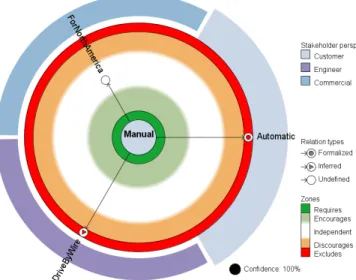
Our visualisation paradigm, called FRoGs, has as objective to visualise the constraints (relations) between features based on the analysis of current configurations. Each FRoG is associ-ated with a specific feature to show how this feature is relassoci-ated, in term of hard and soft constraints, to the other features. A FRoG is presented as a circle where the considered feature is displayed in the center1. This feature in the center will be called fc hereafter . All the rest of features that represent variation points of the FM are displayed around fc with a constant separation of |f eatures|−12π . This separation allows to distribute uniformly all the features around the circle. These features are ordered by stakeholder perspectives so we will have circular sectors for each of the stakeholder perspectives. Before going into the details of the visualisation, Figure 2 shows the FRoG of the Manual feature of the Car example. We can see Manual as fc in the center and the rest of the features separated with a constant angle. We can see also the sectors of the different stakeholders mentioned in the introduction.
1FRoGs acronym is inspired by the metaphor that FRoG graphs have water
lily pond plant shapes and that the domain expert could navigate from one to another
Fig. 2: FRoG for the Manual feature of the Car example
1) FRoG’s zones: Each FRoG displays five zones each of them associated with a specific color and related to a specific type of constraints. Figure 3 shows these zones and how the distance between the fc and the boundary of the circle is calculated according to the figivenfc operation.
• Requires Zone. The Requires zone is reserved to the value 1 and it is the closest to fc. Features in the Requires zone are “glued” to fc meaning that if we have fc then in all EC we have fi. The Requires Zone and the Excludes zone are reserved to only one value and their size fits exactly with the diameter of the fi nodes. The Requires zone is displayed with the green color.
• Excludes Zone. This zone, displayed with the red color, is in the extreme of the circle and therefore is the farthest from the fc to illustrate that fc and fi were not together in any configuration.
• Encourages Zone. This zone includes all fi that are potentially encouraged by the presence of fc. The color is a pale green meaning that it is close to the Requires zone but without reaching it. The Encourages zone fades to white in the Independent Zone at the distance defined by the encthreshold.
• Discourages Zone. This zone includes all fi that are potentially discouraged by the presence of fc. The color is orange meaning that it is close to the Exclude zone but without reaching it. The Discourage zone fades to white in the Independent Zone at the distance defined by the disthreshold.
• Independent Zone. This zone, located between the encthreshold and the disthreshold, is displayed with the white color containing the features that are not impacted by the presence of fc.
In the FRoG of Figure 2 we can see how both Au-tomatic and DriveByWire are in the Excludes zone and ForNorthAmerica (with a figivenfcof 0.5) is located exactly in the middle between the Requires and Excludes zones corresponding to the Independent zone.
The usage of colors in visualisation is an important de-sign decision [27]. FRoG zones depends to univariate data (figivenfc). This data has continuous values but, as we have shown, these values are mapped to zones in a discrete fashion. Therefore, we have defined boundaries and we associate one color to each of the zones following the color scheme shown in Figure 3.
The green of the Requires zone contrasts heavily with the red of the Excludes zone. The separation principle, that claims
that close values must be represented by colors perceived to be closer, is respected with the green and the pale green for the Requires and Encourages zones as well as with the red and the orange colors for the Excludes and Discourage zones. The color scheme used in FRoG’s zones can be seen as a diverging color scheme given that it illustrates the progression from a central point.
Colder colors are perceived to be lower than warmer colors as in the case of heat maps. This is respected in FRoGs taking into account that the distance from fc to the Requires zone is lower than the higher distance to the Excludes zone. In addition, as it happens with the traffic lights metaphor shared by most of the cultural contexts, the red color for the Excludes zone has a connotation of interdiction while the green of the Requires zone has a connotation of being positive.
The size of the Requires and Excludes zones fits exactly with the size of a fi node while the other zone sizes depend on the percentage defined in the encthresholdand disthreshold. The fade from the Encourages and Discourages zones is very small in size and it is aimed only to create a visual effect that these boundaries are not as restrictive as the hard constraints boundaries represented with a black line. For example, a feature fi with a formalized excludes hard constraint cannot appear in the discourages zone because otherwise it was not a hard constraint. On the contrary, one feature fi that has not a hard constraint could “move” between the Encourages, Independent and Discourages zone over time because of the addition of new configurations.
2) Formalized and non formalized constraints: A FRoG displays the mined constraints by analysing the EC. However, some of them (or all in an optimistic case) are normally already defined in the FM. In the FRoG visualisation, for these already formalized constraints we add a circle in the node of fi with the color of the corresponding constraint’s type as shown in Figure 4. For example, M anual ⇒ ¬Automatic is an already formalized constraint and Figure 2 shows this notation on the Automatic node with the red color as it is an Excludes constraint.
Notice that, if we have formalized soft constraints, it could happen that the mining process on EC may situate fi in a FRoG zone that does not correspond to the defined soft constraint. This could alert the user about a general violation of the formalized soft constraint.
Figure 2 shows the FRoG legend at the right side of the image. In this legend, the “Relation types” category shows the notation for other types of feature relations apart from the Formalized relation. We use the grey color in the figures but
Formalized Requires constraint Formalized Excludes constraint Formalized Encourages constraint Formalized Discourages constraint
Fig. 4: Formalized constraints notation
it will be the color of the different constraints and, in any case, grey color. An inferred constraint, as explained before, is a constraint that is not formalized in the FM but that exists because of logical rules. Figure 2 shows an example of it in the DriveByWire node. We use the triangle to differentiate it from the circle of the formalized constraints. The triangle metaphor contrasts with the circle and it has the connotation of an arrowhead representing the existence of a rule of inference. If it is neither a formalized nor inferred constraint, we will refer to it as an undefined relation independently of the zone where the fiis placed. Undefined relations do not contain any symbol inside the fi node.
3) Stakeholder Perspectives: Each stakeholder perspective has an associated color that is used in the circular sectors of the FRoG. The fc node has the color of the stakeholder perspective it belongs to, and also, this circular sector has a slightly bigger radius. Figure 2 shows how the Manual feature has the Customer color and that the Customer sector has bigger radius.
The stakeholder perspectives colors could be changed by users but default colors are provided. Stakeholder perspectives are nominal data and we used a qualitative color scale that does not imply order. Figure 5 shows the used color scheme. In the rejected alternatives section III-E2, it is discussed why only grey, purple and blue variations are present in this default color scheme.
Fig. 5: Default color scheme for the nominal data of stake-holder perspectives
4) Displaying the Confidence: The confidence is displayed outside of the circle as a percentage accompanied by a pie chart visualizing this percentage. In Figure 2 we can see in the bottom-right side a Confidence of 100% and complete black circle. As another example Figure 6 shows the visualisation of the confidence with a value of 5%.
C. Interaction possibilities
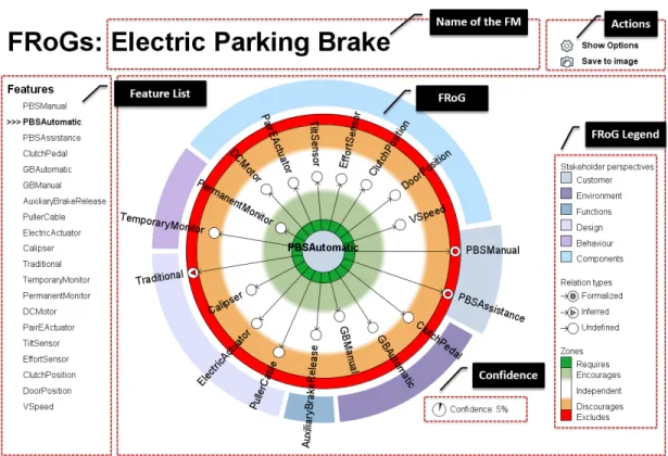
FRoGs was implemented as a visualisation tool allowing free exploration. The navigation and filter capabilities are discussed in the next paragraphs. To illustrate these interaction possibilities, Figure 6 shows a screen-shot of FRoGs visuali-sation tool at which we added dashed sections to differentiate the different parts. The “Name of the FM” part just shows the name of the FM of the SPL while the “Feature List” part contains all the variable features of this FM. The “FRoG” part shows the FRoG of the selected feature with the “Confidence” and “Legend” sub parts. Finally, the “Actions” part activates different interaction capabilities.
1) Navigation: On the left side of Figure 6 we can see the “Feature List” part. A bold font and an arrow is used to distinguish the selected feature. We can click in any feature or use the keyboard to change the displayed FRoG. We can also click in any node of the graph to navigate to the FRoG of the selected feature.
Fig. 6: Screenshot of FRoGs visualisation tool focusing on the PBSAutomatic feature of the Electric Parking Brake SPL
2) Filters: Filters can be applied simultaneously to hide feature nodes of stakeholder perspectives, relation types or FRoG zones. FRoG users should click on the “Show Options” button of the “Actions” part to have access to these function-alities. By clicking this button, checkboxes will appear on the FRoG legend to activate or deactivate the filters as shown in Figure 7. The button “Show Options” text changes to “Hide Options” to hide these functionalities and come back to the purely visualisation operations.
Different filter combinations could fulfil different objectives of FRoGs usage as for example:
• Documenting constraints: We focus on constraints by hiding all features on the Independent zone.
• Discovery of non formalized constraints: We focus on potential constraints by hiding all features on the In-dependent zone and those constraints that are already formalized or inferred.
• Intra-stakeholder perspectives constraints: We hide all the features that do not correspond to a given stakeholder perspective.
• Inter-stakeholder perspectives constraints: We hide all the features that do not correspond to a given set of stakeholder perspectives.
3) Adjusting encourages and discourages thresholds: By clicking in the “Show Options”, apart from the filtering checkboxes, the legend of the zones is transformed in a range slider. Figure 6 shows the initial appearance of the legend of the zones at the bottom of the “Frog Legend” part, and Figure 7 shows the legend of the zones enriched with the
Fig. 7: Filtering options and slider for adjusting encourages and discourages thresholds
slider functionality and with a textual representation of the selected percentages. Using this slider, the encthreshold and disthreshold could be adjusted at will. Interacting with the slider provides automatic feedback in the FRoG by changing the size of the zone. If filters are applied to the feature nodes, these filters have also effect so hidden nodes could appear or disappear while interacting with the slider.
4) Save as image: Another interaction capability of the visualisation tool is a button to save the current FRoG (fil-tered or not fil(fil-tered) and the legend to an image file. This functionality is available in the “Actions” part of Figure 6. The “Name of the FM”, “Actions” and “Feature List” parts are not appearing in the saved image and therefore it can be used directly for documentation or to illustrate some phenomena in feature relations.
D. Time response
FRoGs was implemented with Processing 2.0 [8] and we achieve complete visual continuity. figivenfj is an algorithm with order O(m) where m is the number of existing con-figurations. Therefore, displaying a FRoG is O(nm) being n the number of features. The number of possible valid configurations is precomputed before starting the visualisation. The needed set of input files for FRoG are exported using the SPL tool Feature IDE [29] and the mapping from stakeholder perspectives to features are defined in another configuration file.
E. Rejected alternatives
1) Colors of Requires and Excludes zones: In the beginning we used pale green and pale red for the Requires and Excludes zones but users reported that they will prefer more intense green and red colors for these zones to catch more attention on hard constraints.
2) Default colors for stakeholder perspectives: Qualitative scales for nominal data are publicly available as for example the color scheme provided by ColorBrewer 2.0 [7] shown in Figure 8. We started using this color scheme but users complained about the similarities between some of the colors of the stakeholder perspectives’ sectors and the red of the Excludes zone. For instance, the fourth color of Figure 8 was a cause of confusion. We decided to exclude those colors that were similar to red, orange as well as similar to green and pale green.
Fig. 8: Rejected default color scheme for the nominal data of stakeholder perspectives
3) Relation types: The current version of FRoGs only has the possibility to see the impact of the presence of fc in the presence of the other features fi. In order to display other phenomena in the relations of a given feature fc, FRoGs im-plementation was flexible to show the impact of the presence or absence of fc in the presence or absence of other features fi. It was also available to show the impact of the presence or absence of the rest of the features fiin relation with fc. These aspects give raise to eight possible FRoGs for a given fcfrom which Figure 9 shows four of them that could be obtained from a given fc.
How the presence of fcaffects the presence of others
How the presence of others affects the presence of fc
How the absence of fcaffects the presence of others
How the absence of others affects the presence of fc
Fig. 9: Different relations regarding presence or absence of features, and the direction of the relation regarding the FRoG central feature
The other four combinations could also be displayed even if they are the “inverse” of one of these four types because of the following property of the figivenfj operation: figivenfc = 1 − (¬fi)givenfc. Notice that the direction of the arrows from fc to fi changes in types one and two, and three and four. To obtain the distances in the cases that we want to show the impact of other features on fc, it is enough to inverse the figivenfj operation: For type one is figivenfcwhile for type two is fcgivenfi.
This functionality in the options of the visualisation tool gave raise to many confusion in the users. It is not easy to think about presence and absence of features in combination with the direction of the arrows. Our case study did not need these kinds of relation visualisation for documentation nor for constraint discovery so we decided to remove it for easing FRoGs usage until we prove its usefulness in some scenario. Current version of FRoGs visualisation corresponds to the first type of Figure 9 as shown for example in Figure 2.
IV. CASE STUDY AND DISCUSSIONS
In the previous sections we illustrated FRoGs on the Car example. In this section we present FRoGs evaluation on an industrial case study in the automotive industry concerning the Renault’s Electric Parking Brake (EPB) SPL [13], [20]. First we describe the case study and then we discuss the results. A. Case Study: Electric Parking Brake
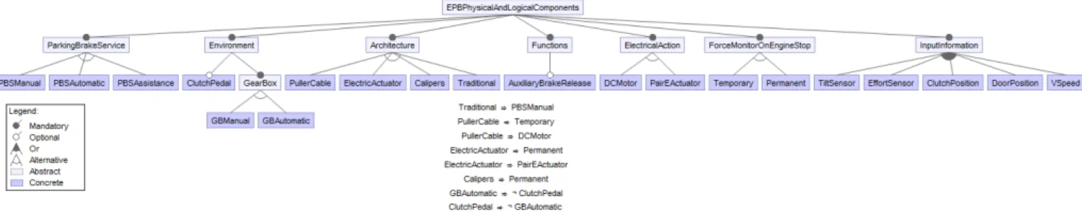
The EPB system is a variation of the classical, purely mechanical, parking brake, which ensures vehicle immobi-lization when the driver brings the vehicle to a full stop and leaves the vehicle. The case study is focused on the variability in the BOM (Bill of Materials) related to the logical/physical components of the EPB. Figure 10 presents the FM specified by domain experts. This FM contains 20 variable features and 32 hard constraints. In concrete, the Alternative constructions between features define 24 hard constraints and 8 are expressed as logical expressions. The possible valid configurations of this FM are 2976 while the existing configurations that were provided are 200.
The variability in this SPL is described by Renault ac-cording to six stakeholder perspectives that represent differ-ent subdomains of the EPB’s variability. These stakeholder perspectives are Customer, Environment, Functions, Design, Behavior and Components. We present here a brief description of these perspectives and their associated features.
a) Customer: Customer visible variability is handled by the product division. For customers, the parking brake proposes three types of services: The manual brake is con-trolled by the driver either through the classical lever or a switch; the automatic brake is a system that may enable or disable the brake itself depending on an automatic analysis of the situation; the assisted brake comes with extra functions which aid the driver in other situations such as assistance when starting the car on a slope. The features concerned by this perspective are thus PBSManual, PBSAutomatic and PBSAssisted.
Fig. 10: Electric Parking Brake system Feature Model for physical and logical components
b) Environment: For vehicle environment, the variability concerns the Gear Box where we distinguish two possible variants: GBManual and GBAutomatic. The presence of a ClutchPedal is also an optional feature.
c) Functions: The feature AuxialiaryBrakeRelease is re-lated to an optional function of the system that includes an auxiliary brake release mechanism.
d) Design: There are different alternatives that concern design decisions of the EPB. These design decisions impact the whole or parts of the technical solution. For architectural design, there are four feature alternatives: PullerCable, Elec-tricActuator, Calipser and TraditionalPB.
e) Behavior: Braking pressure is monitored after the vehicle has stopped for a certain amount of time for the single DC motor or permanently monitored for other solutions. The Behaviour includes thus the features TemporaryMonitor and PermanentMonitor.
f) Components: The variability in the EPB also concerns the physical architecture/components. This consists in the presence of different means of applying the brake force: electric actuators mounted on the calipers or single DC motor and puller cable much like the traditional mechanical parking brake. Also the type of sensors available may vary depending on the configuration and needs. This perspective thus includes the following features: DCMotor, PairEActuator, TiltSensor, EffortSensor, ClutchPosition, DoorPosition, and VSpeed.
B. Results: FRoGs of the Case Study
From the 200 existing configurations of the EPB case study we obtained 20 FRoGs, one per feature. Figure 6 shows these features in the “Feature List” part. Table II shows the informa-tion that can be visualised on the FRoG of each feature. For each FRoG’s central feature, the table shows the number of constraints that can be identified by analysing the different zones. Regarding the soft constraints, the values used for encthershold and disthershold are 25% and 75% respectively. Figure 6 shows the PBSManual FRoG, that corresponds to the second element in Table II, where we can see that it displays 2 hard constraints, 1 inferred, and 4 potential soft constraints. Before experimenting with domain experts, we manually checked the correctness of the visualised information. Con-cretely, we checked manually that the formalized hard and inferred constraints of the FM appear in the displayed FRoGs.
TABLE II: Number of the identified constraints using FRoGs FRoG central feature Hard Inferred Soft
PBSManual 2 0 2 PBSAutomatic 2 1 4 PBSAssistance 2 1 3 ClutchPedal 1 1 4 GBAutomatic 2 0 4 GBManual 1 0 4 AuxiliaryBrakeRelease 0 0 4 PullerCable 5 2 0 ElectricActuator 5 2 0 Calipser 4 1 0 Traditional 4 2 0 TemporaryMonitor 1 2 2 PermanentMonitor 1 1 1 DCMotor 1 1 3 PairEActuator 1 1 3 TiltSensor 0 0 5 EffortSensor 0 0 4 ClutchPosition 0 0 4 DoorPosition 0 0 4 VSpeed 0 0 4 Total 32 15 55 Average 1.6 0.75 2.75 Standard Deviation 1.67 0.79 1.68
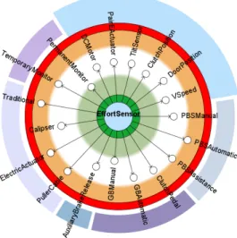
We discuss now some analysis that domain experts made using FRoGs and how it helps in the comprehension of feature relations in the EPB SPL. For instance, analysing the FRoG associated with the EffortSensor feature (see Figure 11), it is observed that it has no hard constraints to any other features. That means that it has no hard impact on the presence or absence of any feature. However, the feature PullerCable (see Figure 12) has a great impact on other features as the PullerCable FRoG shows seven features on the Excludes and Requires zones.
No undefined hard constraints were found neither in the Excludes nor Requires zones in EPB’s FRoGs. However, thanks to FRoGs, as shown in Table II, 55 potential soft constraints are displayed. By visualising this, domain experts are able to think about two possibilities: a) whether it is an actual soft constraint that should be formalized or b) FRoG displayed a fact based on the existing configurations but it is not an actual soft constraint. The exercise also enables to think about the thresholds for the Encourages and Discourages zones.
The FRoGs for the EPB’s FM also represented a visualisa-tion paradigm to understand the relavisualisa-tions between stakeholder perspectives. From the 47 hard or inferred constraints, 20 of them are hard constraints that relate features belonging to
Fig. 11: FRoG of EffortSensor feature without filters showing that it does not representatively affect other features
Fig. 12: FRoG of PullerCable feature with a filter hiding Independent zone features to illustrate great impact on other features
different stakeholder perspectives. Figure 12 shows 4 inter-stakeholder perspectives hard constraints: TemporaryMonitor, PermanentMonitor, DCMotor and PairEActuator. In addition, in the case of soft constraints, the 55 soft constraints are between inter-stakeholder perspectives. Figure 11 shows 4 of them: PullerCable, ElectricActuator, PermanentMonitor and PBSAutomatic.
V. RELATEDWORK
As presented above, the FM is classically visualised as a tree structure consisting of features. Constraints between these features are displayed using the Alternative and the Or variability notation. Constraints (e.g.; requires, excludes) can also be explicitly formalized textually (Figure 10) as logical expressions or graphically (Figure 1) as arrows between features [16], [25]. As discussed in this paper, real-world SPLs yield FMs that can be large and complex with many
constraints. Hence, it is difficult to use this representation to help domain experts to understand relations between features. In recent years, the use of visualisation techniques in the SPL community has received a lot of attention proposing new alter-natives to visualise FMs. Trinidad et al. [30] proposed the cone tree visualisation paradigm introducing a 3D representation of FMs. However, this visualisation is only proposed to represent the hierarchical information included in large FM and the authors do not consider constraint visualisation.
SPL visualisation related work mainly consider the use of visualisation techniques to help domain experts for prod-uct configuration. Prodprod-uct configuration is the process that consists in selecting, from the FM, the list of features that will be included in the target configuration. Visualisation is often combined with interactive techniques to support product configuration. A survey on the use of visualisation techniques for product configuration is presented in [23]. Nestor et al. [21] propose a tool called VISIT-FC (Visual and Interactive Tool for Feature Configuration) that introduces visualisation techniques to address product configuration. For constraint visualisation, this tool only uses arcs between features. Constraints are also visualised as arcs in the S2T2 visualisation tool [22]. [4] also discuss product configuration but without considering constraint visualisation. In [17], the authors propose the use of visualisation techniques to display features for pairwise testing but constraints are not visualised. On the contrary, we propose FRoGS as a new formalism to visualise constraints between features. Instead of classical representations where constraints are integrated in FMs and often visualised as arcs between features, FRoGs display the constraints focusing on relations of each feature with the rest of the features. This allows to study the impact of each feature on the rest of the FM. At our best knowledge FRoGs represent the first work in this direction.
In Section III, we presented our approach to extract con-straints and build FRoGs from existing configurations. Extract-ing constraints from sets of configuration has received a lot of attentions in the context of reverse engineering of feature models [14]. Many papers [9], [12], [15], [18], [19], [26], [31] in this context propose algorithms to extract constraints from existing configurations. However, all these algorithms only extract constraints without proposing any visualisation mechanisms. Our main objective by introducing FRoGs is not to propose a new extraction algorithm but to contribute a formalism to visualise the mined constraints. Thus, FRoGs can be used as a front-end to visualise constraints using any algorithm.
FRoGs visualisation can be categorized as a radial ego network representation. The ego represents the focal node of the graph. This approach has been used mainly in social network analysis. In software engineering, ego networks has been proposed to visualise how the modification of a given component could demand the evolution of the other compo-nents [11] based on the version control system information. FRoGs use ego network representations but it is designed to deal with the specificities of feature relations in SPLE.
VI. CONCLUSION& FUTUREWORK
Feature constraints are the core of Feature Models and identifying and maintaining them is challenging in Software Product Line engineering. This paper proposes a new paradigm called FRoGs to help domain experts to visualise in an interactive way the feature relations mined from existing configurations. This can help to potentially refine an existing feature model by formalizing new hard and soft constraints. In addition, FRoGs can be used to document, at the domain level, each feature by displaying its relations among the rest of features. We demonstrate in this paper the usability of FRoGs on a real-world case study from a major manufacturer.
Our future work has two main directions: 1) Regarding to visualisation, FRoGs can be improved to consider the time dimension. Indeed, the time dimension in the creation of each existing configuration could help users to understand the dynamicity on feature relations and reason about feature obsolescence or usage over time. 2) Independently from the visualisation aspect, we aim to improve the way that FRoGs are built by providing heuristics for default values for the encourage and discourages thresholds.
AKNOWLEDGMENTS
We would like to thank the Renault company for provid-ing the information for the case study and participatprovid-ing in the improvement of the visualisation. The present work is supported by the Fonds National de la Recherche (FNR), Luxembourg, under the project MODEL C12/IS/3977071 and the AFR grant agreement 7898764. The work of Tewfik Ziadi was also supported by the University of Luxembourg as a visiting researcher.
REFERENCES
[1] D. S. Batory. Feature models, grammars, and propositional formulas. In J. H. Obbink and K. Pohl, editors, SPLC, volume 3714 of Lecture Notes in Computer Science, pages 7–20. Springer, 2005.
[2] D. Benavides, P. Trinidad, and A. Ruiz-Cort´es. Automated reasoning on feature models. In LNCS, Advanced information systems engineering: 17th international conference, CAISE 2005. Springer, 2005.
[3] D. Beuche. Modeling and building software product lines with pure::variants. In SPLC Workshops, page 296, 2010.
[4] G. Botterweck, M. Janota, and D. Schneeweiss. A design of a configurable feature model configurator. In D. Benavides, A. Metzger, and U. W. Eisenecker, editors, VaMoS, volume 29 of ICB Research Report, pages 165–168. Universit¨at Duisburg-Essen, 2009.
[5] S. B¨uhne, G. Halmans, and K. Pohl. Modeling dependencies between variation points in use case diagrams. In Proceedings of 9th intl. Workshop on Requirements Engineering - Foundations for Software Quality, pages 59–69, 2003.
[6] S. K. Card, J. D. Mackinlay, and B. Shneiderman, editors. Readings in Information Visualization: Using Vision to Think. Morgan Kaufmann Publishers Inc., San Francisco, CA, USA, 1999.
[7] Colorbrewer. Colorbrewer2, color advice for cartography. http://colorbrewer2.org.
[8] A. Colubri and B. Fry. Introducing processing 2.0. In SIGGRAPH Talks, page 12. ACM, 2012.
[9] K. Czarnecki, S. She, and A. Wasowski. Sample spaces and feature models: There and back again. In SPLC, pages 22–31. IEEE Computer Society, 2008.
[10] K. Czarnecki and A. Wasowski. Feature diagrams and logics: There and back again. In SPLC, pages 23–34. IEEE Computer Society, 2007. [11] M. D’Ambros, M. Lanza, and M. Lungu. The evolution radar:
Visu-alizing integrated logical coupling information. In Proceedings of the International Workshop on Mining Software Repositories, 2006.
[12] J.-M. Davril, E. Delfosse, N. Hariri, M. Acher, J. Cleland-Huang, and P. Heymans. Feature model extraction from large collections of informal product descriptions. In ESEC/SIGSOFT FSE, pages 290–300, 2013. [13] C. Dumitrescu, R. Mazo, C. Salinesi, and A. Dauron. Bridging the gap
between product lines and systems engineering: An experience in vari-ability management for automotive model based systems engineering. In Proceedings of the 17th International Software Product Line Conference, SPLC ’13, pages 254–263, New York, NY, USA, 2013. ACM. [14] W. Fenske, T. Th¨um, and G. Saake. A taxonomy of software product
line reengineering. In P. Collet, A. Wasowski, and T. Weyer, editors, VaMoS, page 4. ACM, 2014.
[15] E. N. Haslinger, R. E. Lopez-Herrejon, and A. Egyed. On extracting feature models from sets of valid feature combinations. In V. Cortellessa and D. Varr´o, editors, FASE, volume 7793 of Lecture Notes in Computer Science, pages 53–67. Springer, 2013.
[16] K. C. Kang, S. G. Cohen, J. A. Hess, W. E. Novak, and A. S. Peterson. Feature-oriented domain analysis (foda) feasibility study. Technical report, DTIC Document, 1990.
[17] R. E. Lopez-Herrejon and A. Egyed. Towards interactive visualization support for pairwise testing software product lines. In A. Telea, A. Kerren, and A. Marcus, editors, VISSOFT, pages 1–4. IEEE, 2013. [18] R. E. Lopez-Herrejon, J. A. Galindo, D. Benavides, S. Segura, and
A. Egyed. Reverse engineering feature models with evolutionary algorithms: An exploratory study. In G. Fraser and J. T. de Souza, editors, SSBSE, volume 7515 of Lecture Notes in Computer Science, pages 168–182. Springer, 2012.
[19] A. Lora-Michiels, C. Salinesi, and R. Mazo. A method based on association rules to construct product line models. In D. Benavides, D. S. Batory, and P. Gr¨unbacher, editors, VaMoS, volume 37 of ICB-Research Report, pages 147–150. Universit¨at Duisburg-Essen, 2010. [20] R. Mazo, C. Dumitrescu, C. Salinesi, and D. Diaz. Recommendation
heuristics for improving product line configuration processes. In Rec-ommendation Systems in Software Engineering, pages 511–537. 2014. [21] D. Nestor, S. Thiel, G. Botterweck, C. Cawley, and P. Healy. Applying
visualisation techniques in software product lines. In SOFTVIS, pages 175–184, 2008.
[22] A. Pleuss and G. Botterweck. Visualization of variability and configu-ration options. STTT, 14(5):497–510, 2012.
[23] A. Pleuss, R. Rabiser, and G. Botterweck. Visualization techniques for application in interactive product configuration. In I. Schaefer, I. John, and K. Schmid, editors, SPLC Workshops, page 22. ACM, 2011. [24] K. Pohl, G. B¨ockle, and F. J. v. d. Linden. Software Product Line
Engineering: Foundations, Principles and Techniques. 2005.
[25] P.-Y. Schobbens, P. Heymans, and J.-C. Trigaux. Feature diagrams: A survey and a formal semantics. In Requirements Engineering, 14th IEEE international conference, pages 139–148. IEEE, 2006.
[26] S. She, R. Lotufo, T. Berger, A. Wasowski, and K. Czarnecki. Reverse engineering feature models. In R. N. Taylor, H. Gall, and N. Medvidovic, editors, ICSE, pages 461–470. ACM, 2011.
[27] S. Silva, B. S. Santos, and J. Madeira. Using color in visualization: A survey. Computers & Graphics, 35(2):320 – 333, 2011. Virtual Reality in Brazil Visual Computing in Biology and Medicine Semantic 3D media and content Cultural Heritage.
[28] J. Sincero, R. Tartler, C. Egger, W. Schr¨oder-Preikschat, and D. Lohmann. Facing the linux 8000 feature nightmare. In Proceedings of ACM European Conference on Computer Systems (EuroSys 2010), Best Posters and Demos Session, 2010.
[29] T. Th¨um, C. K¨astner, F. Benduhn, J. Meinicke, G. Saake, and T. Leich. FeatureIDE: An extensible framework for feature-oriented software development. Science of Computer Programming, 79(0):70 – 85, 2014. Experimental Software and Toolkits (EST 4): A special issue of the Workshop on Academic Software Development Tools and Techniques (WASDeTT-3 2010).
[30] P. Trinidad, A. R. Cort´es, D. Benavides, and S. Segura. Three-dimensional feature diagrams visualization. In S. Thiel and K. Pohl, editors, SPLC (2), pages 295–302. Lero Int. Science Centre, University of Limerick, Ireland, 2008.
[31] K. Yoshimura, Y. Atarashi, and T. Fukuda. A method to identify feature constraints based on feature selections mining. In SPLC (2), pages 425– 429, 2010.
[32] Y. Yu, J. C. S. do Prado Leite, A. Lapouchnian, and J. Mylopoulos. Configuring features with stakeholder goals. In R. L. Wainwright and H. Haddad, editors, SAC, pages 645–649. ACM, 2008.
![Fig. 1: Example of Car Feature Model. Credits to Czarnecki et al. [9]](https://thumb-eu.123doks.com/thumbv2/123doknet/13012448.380717/2.918.510.806.938.1037/fig-example-car-feature-model-credits-czarnecki-et.webp)