Axis detection of cylindrical objects in 3-D images

HAL Id: hal-00326703

https://hal.archives-ouvertes.fr/hal-00326703

Submitted on 5 Oct 2008

HAL is a multi-disciplinary open access archive for the deposit and dissemination of

sci-L’archive ouverte pluridisciplinaire HAL, est destinée au dépôt et à la diffusion de documents

Axis detection of cylindrical objects in 3-D images

Christianne Mulat, Marc Donias, Pierre Baylou, Gérard Vignoles, Christian

Germain

To cite this version:

Christianne Mulat, Marc Donias, Pierre Baylou, Gérard Vignoles, Christian Germain. Axis detection of cylindrical objects in 3-D images. Journal of Electronic Imaging, SPIE and IS&T, 2008, 17 (3), pp.0311081-0311089. �hal-00326703�

Axis detection of cylindrical objects in 3-D images

Christianne Mulat (mulat@lcts.u-bordeaux1.fr)

LCTS, UMR 5801 CNRS-UB1-Safran-CEA,

3 allée La Boëtie, Domaine Universitaire, 33600 Pessac, France. Marc Donias (marc.donias@laps.ims-bordeaux.fr)

IMS, Dept. LAPS, Equipe Signal et Image, UMR 5218 CNRS ENSEIRB, Batiment A4, 351 cours de la libération, 33405 Talence, France.

Pierre Baylou

IMS, Dept. LAPS, Equipe Signal et Image, UMR 5218 CNRS - ENSEIRB, Batiment A4, 351 cours de la libération, 33405 Talence, France.

Gérard Vignoles (vinhola@lcts.u-bordeaux1.fr)

LCTS, UMR 5801 CNRS-UB1-Safran-CEA,

3 allée La Boëtie, Domaine Universitaire, 33600 Pessac, France. Christian Germain (christian.germain@laps.ims-bordeaux.fr)

IMS, Dept. LAPS, Equipe Signal et Image, UMR 5218 CNRS –ENITAB, Batiment A4, 351 cours de la libération, 33405 Talence, France.

ABSTRACT

This paper introduces an algorithm dedicated to the detection of the axes of cylindrical objects in a 3-D block. The proposed algorithm performs the 3-D axis detection without prior segmentation of the block. This approach is specifically appropriate when the grey levels of the cylindrical objects are not homogeneous and thus difficult to distinguish from the background. The method relies on gradient and curvature estimation and operates in two main steps. The first one selects candidate voxels for the axes and the second one refines the determination of the axis of each cylindrical object. Applied to fiber reinforced composite materials, this algorithm allows detecting the axes of fibers in order to obtain the geometrical characteristics of the reinforcement. Knowing the reinforcement characteristics is an important issue in the quality control of the material but also in the prediction of the thermal and mechanical performance. In this paper, the various steps of the algorithm are detailed. Then, some results are presented, obtained with both synthetic blocks and real data acquired by synchrotron X-ray micro tomography on carbon-fiber reinforced carbon composites.

1. INTRODUCTION

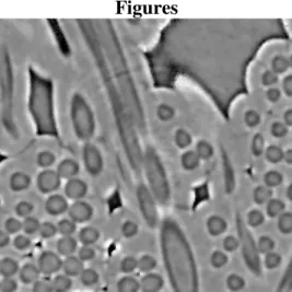
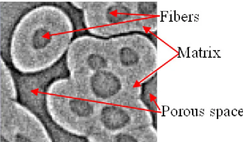
Composite materials (Figure 1) are increasingly used in many industrial applications. These materials usually consist in the combination of a matrix providing a coating on a reinforcement made of cylindrical fibers. The reinforcement geometry is one of the most significant properties in order to assess the mechanical and thermal behavior of a composite material. Among the relevant geometrical characteristics of reinforcement, one can quote its fiber location, diameter, orientation, or curvature. These characteristics can also be used as a priori data for 2-D or 3-D numerical predictions of the thermal and mechanical performances of the material. Even if some of these

geometrical characteristics can be estimated using 2-D imaging techniques[1], 3-D data offer a more

extensive characterization of the reinforcement [2]. Estimation of geometrical properties of cylinders in a 3-D block has also been studied in other contexts, such as medical imaging [3].

Estimating the geometrical properties of cylindrical objects in 3-D blocks can be achieved using either top-down or bottom-up approaches. Top-down approaches consist of three steps:

• Separation of the cylinders from the “background” of the 3-D block; this step is usually done using segmentation techniques.

• Labeling of each cylinder.

• Estimation of geometrical properties of each cylinder; mathematical morphology operators such as thinning or 3-D skeletonizing [4], or other approaches like Hough transform [5] can help to fulfill this task.

On another hand, bottom-up approaches consist in directly extracting the axes from the 3-D data. Then, knowing the axes, orientation, curvature and location of the cylinders can be estimated. Even the reinforcement volume ratio can be obtained from the axes detection if the cylinder radii are a

priori known. Otherwise, a segmentation step based on region growing [6] or active contours [7],[8] can be done, using the known axes locations and orientations as an initialization step.

This paper is focused on the bottom-up approaches which are specially attractive if the segmentation of the fibers is difficult or if the knowledge provided by the axis is sufficient to characterize the material.

Most algorithms dedicated to axis detection of tubular structures are related to medical imaging, for vessel segmentation purposes [3], [9-13]. The axis detection step of these methods relies on the computation of eigenvectors or eigenvalues (ur₁,

λ

₁; ur₂,

λ

₂; ur₃,

λ

₃ with

λ

₁>

λ

₂>

λ

₃) of the Hessian matrix. On one hand, the eigenvectors provide with the orientation across and along to the line structure [9]. Line detection filters can then be processed along the expected line direction. On another hand, the eigenvalues reflecting the second derivative of the grey level profile, they indicate the kind of local geometrical structure (plane, line…) of which a voxel belongs [10-12]. In 2000, Krissian [3] improved these methods taking into account the local gradients. At first, using the eigenvalues (

λ

₂,

λ

₃), Krissian selects voxels expected to be close to the vessel axis. Then, for each selected voxel, a circle is defined in the plane given by the eigenvectors ur₂, ur₃. The circle is centered on the current selected voxel, and its radius can vary, thus allowing a multi-scale scheme. The local gradients of the grey levels, computed on these circles, provide a response function of which the local maxima are expected to be axis voxels.

This method relies on a strong hypothesis regarding the grey level section profile of the tubular structures. Indeed, the selection rule of the axis candidate voxels (

λ

₂ < and 0

λ

₃< ), relies on a 0 Gaussian profile assumption. For more complex, but realistic profile functions, this assumption is not valid. Furthermore, the local gradient computation in the cross section plane (ur₂, ur₃) requires trilinear interpolations, since the cross section plan usually do not line up on the voxel grid. Finally, the multiscale scheme is not useful when the cylindrical structure radius is even roughly known, since the cylinder radii can then be accurately derived from the local curvature estimation.

Therefore, a new approach for cylindrical object axis detection is proposed. It allows obtaining directly from gradient and curvature information the radius and the orientation of the cylindrical objects and aims at avoiding the shortcomings mentioned above.

In the second section, the various steps of this approach are explained. The third section presents some results, first for synthetic 3-D blocks and then for experimental data acquired on fiber-reinforced composite materials.

2. AXIS DETECTION PROCESS

The approach dedicated to the axis detection algorithm begins with an initialization step, mainly devoted to local gradient estimation. Then, it features two main steps (Figure 2), a coarse one and a fine one. The coarse step selects a set of candidate voxels for each axis. The fine step, starting from the previous set, determines the axis of each cylindrical object of the 3-D block.

2.1 Initialization

The objects of interest are supposed to be, at least locally, cylindrical isosurfaces centered on the real axis of the cylinder. In order to reduce the computation time, only the voxels belonging to a cylindrical isosurface are used for the next steps (Figure 2). To determine whether or not a voxel belongs to a cylindrical isosurface, a thesholding on the gradient norm is applied. The grey level variation induced by the noise being usually weaker than the object profile grey level variation, this threshold is manually tuned according to the noise level in the block. However, the value of the threshold is not critical and can be underestimated without major effect on the results. Indeed, since the gradients induced by the noise are not coherent in orientation, the structure tensor (section 2.2) will reduce the noise contribution to the axis orientation estimation. The resulting set of selected gradients is used as input data for the coarse stage of the axis detection process.

Classical gradient masks can be found in the literature. Among them, Prewitt, Sobel or cross gradient masks are frequently used with 2-D images and can be easily extended to 3-D. However, they are not well adapted to orientation estimation in the case of cylindrical objects as they provide biased estimation. Other gradient estimators [14] have been optimized regarding some specific purpose, such as detecting a step profile in 1-D or 2-D data corrupted by white Gaussian noise.

Herein, in order to optimize the axis detection process, a specific gradient-based optimal operator dedicated to accurate estimation of the direction toward the axis is proposed.

The masks are estimated in 2-D case, for the detection of the center of disk objects, and then extended in 3-D case, for the estimation of the direction toward the axis of a cylinder.

The gradient estimation scheme relies on the modeling of the 1-D profile function of the cylinder, i.e. the evolution of the voxel intensity f(r) versus the radius r. Monomial profile functions have been

considered: _{( )}

(

2 2 2

)

n

f r = x +y +z , with (x,y,z) being the voxel coordinates and n the order of the

profile function. Expressing the convolution between the gradient mask coefficients and the profile function gives no bias constraints. These constraints, associated with noise sensitivity considerations, allow computing the optimized gradient mask coefficients. The optimization scheme is detailed in [15]. The resulting 3-D convolution masks, m_x, m_yand m_z are referred to as G3D10 (Figure 3).

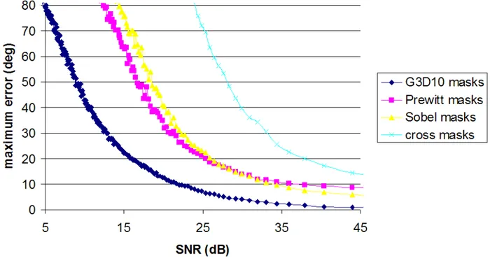
G3D10 masks offer unbiased estimations of the orientation toward the axis when the cylindrical object axis coincides with one the mask reference axis and for even order n for the profile function. In the general case, i.e. oblique cylinders and for any profile function, G3D10 masks still provide better estimations than Prewitt, Sobel or cross masks, thus appearing less biased and more robust with respect to noise influence than classical gradient operators (Figure 4). More results regarding G3D10 can be found in [15].

2.2 Coarse stage: selection of candidate voxels Orientation estimation

The G3D10 masks give the estimation of the gradient for each voxel belonging to a cylindrical isosurface. An orientation tensor [16] is then applied on the resulting gradient. For each voxel, this tensor consists in the correlation matrix built using gradient vectors neighboring the current voxel. From this tensor, the eigenvalues

λ

₁,

λ

₂,

λ

₃ with

λ

₁>

λ

₂ >

λ

₃, and corresponding eigenvectors

3 2 1,u ,u

ur r r are computed. Thus, the tensor provides the orientation ur₁ toward the axis, but also the orientation ur₃ of the axis (see Figure 5). Moreover, a coplanarity index

µ

= f(

λ

₁,

λ

₂,

λ

₃) is derived from the eigenvalues. It will be used later as a confidence index in order to favor the orientations estimated from coplanar vectors.

Distance to the axis

For each voxel belonging to a cylindrical isosurface, using the orientation toward the axis, it is possible to estimate the distance between this voxel and the corresponding cylinder axis. For this purpose, the Hessian matrix H is built using the vectors ur₁=

(

I I_x, _y,I_z

)

in the neighborhood of the voxel under consideration:

          = zz zy zx yz yy yx xz xy xx I I I I I I I I I H (1) with i I I_i ∂ ∂ = ; j i I I_ij ∂ ∂ ∂ = 2 ; i, j =x,y,z.

(

2 2

)

1 1 max ( ) 4( ) 2 T T T T T n k = − a Ha+b Hb± a Ha−b Hb + a Hb   

(

2 2

)

2 1 min ( ) 4( ) 2 T T T T T n k = − a Ha+b Hb± a Ha−b Hb + a Hb    (2) with: _{2 2 2 2 2} 2 1 ( ) 4 y z x z x y z y z x y I I a I I I I I I I I I     = _− _ + + + _{ } −   r and b=a∧u₁ r _{r r}

(∧ denotes the vectorial product).

The distance to the axis

1

1

n

k

R= is then obtained from the maximal principal curvature.

The minimal principal curvature k_n2 is not used for the detection of cylinder axes but it can provide with useful knowledge about the local warping of the cylindrical object.

Candidate voxels of the axis and average orientation

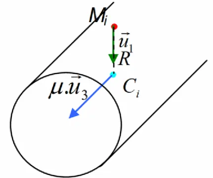
Thanks to the previous steps, the knowledge, for each voxel M belonging to a cylindrical isosurface delivers a set of candidate locations C_ifor the axis, given its orientation ur₁ toward the axis and distance R to the axis (Figure 6).

1 u R C Mi i r × = (3)

The pair (

µ

,ur₃)is then associated to the nearest voxel from the candidate location. With this approach, each voxel M of a cylinder provides the information (

µ

,ur₃)to one candidate voxel Ci.

Thus, a candidate voxel Ci will be related to many cylinder voxels M, and with their associated pair

) ,

(

µ

ur₃ . Therefore, for each candidate voxel Ci, the following tensor (4) is built in order to take all

pairs (µ ,ur₃) into account during the estimation of the axis orientation.

∑

ℑ ∈ _          × × × × × × × × × × × × × × × × × × = M z z z y z x y z y y y x x z x y x x c c c M u M u M M u M u M M u M u M M u M u M M u M u M M u M u M M u M u M M u M u M M u M u M z y x MatC i i i ) ( ) ( ) ( ) ( ) ( ) ( ) ( ) ( ) ( ) ( ) ( ) ( ) ( ) ( ) ( ) ( ) ( ) ( ) ( ) ( ) ( ) ( ) ( ) ( ) ( ) ( ) ( ) , , ( 3 3 3 3 3 3 3 3 3 3 3 3 3 3 3 3 3 3

µ

µ

µ

µ

µ

µ

µ

µ

µ

(4)

with ℑ is the initial set of voxels belonging to cylindrical isosurfaces

This tensor provides an average orientation axis_iof the various vectors used for its construction.

Labeling the candidate voxels

At this stage, the candidate voxels of a given axis form a connected component. Therefore, a hybrid object labeling is carried out [18]. This hybrid labeling combines recursion with iterative scanning and can be directly substituted into any program already using recursion technique. Compared with other methods, recursive or not, performance are improved and speed increased.

Each cylindrical object can then be processed independently through this connected component. In the case of perfect cylinders, the connected components match exactly the cylinder axes. Unfortunately, noise and shape distortion can yield some perturbations. In this case, the connected components are thicker and form elongated clouds inside which the axis is supposed to lie.

2.3 Fine stage: Axis detection

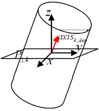
The aim of this stage is to find, inside each connected component, the axis of the corresponding cylinder. For this purpose, the axis going through the center of gravity of each cross-section of a given connected component is assumed to correspond to the real axis of the cylindrical object. As connected components may be bent, the axis detection can not result from a linear regression directly computed from the connected component. Therefore, an approach which detects the axis voxel by voxel has been preferred. For a similar purpose, Krissian [3] proposes, for each selected voxel, to consider the cross section plane of the tubular object. However, since the cylinder axis does not usually match any of the reference frame axes (Figure 7), working with such a cross section requires many trilinear interpolations and increases significantly the computing cost. In order to avoid this computational burden, the estimation is done using the most orthogonal plane to the cylinder axis. The current axis point (xG,yG,zG) is then estimated by computing the center of gravity of the connected component voxels Mi =(xi,yi,zi)which belong to the most orthogonal plane P⊥k to the axis vector

1 −

k

G

axis chosen in

{

xy,xz,yz

}

. For each axis point, the corresponding orientation is estimated by averaging the orientations axis_i of the voxels used to estimate this center (Figure 8).

∑

∑

∑

∑

∑

∑

= = = i i i i i G i i i i i G i i i i i G m z m z m y m y m x m x , , with m_i = axe_i (5)

For each connected component, the recursive approach is applied starting from one extremity of the component. Then, it operates plane by plane all along the connected component, taking benefits of the results (center and orientation) of the previous stage.

3. RESULTS 3.1 Synthetic cylindrical object

In order to validate this approach, a synthetic 3-D block containing one cylinder has been built. As no assumption has been made on the profile function f(d) of the cylinders, Bernstein functions are used, since they are sufficiently general and allow testing various situations:

(

)

(

)

n k 0 1 if ( ) exp -k n k k n n d d a d r k r r f d a

α

d - r otherwise − =  _{     } − ≤       =       

∑

(6)

where d is the axis distance, nis the order of the Bernstein function,

α

a positive parameter and ! !( )! n n k k n k   =   −

  are the binomial coefficients.

The a_kvalues are chosen in order to obtain realistic profile functions, considering fiber grey level profiles. In this paper, the a_kvalues are a₀ =1.5,a_i =1 with i=1..6,a₇ =4,a₈ =1.25, and

8 , 5 . 0 = = n α .

Comparison with Krissian approach

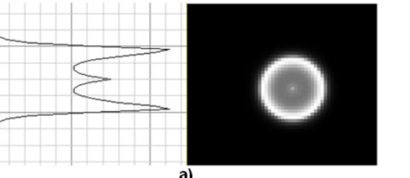
The first step of Krissian approach consists in pre-selecting voxels that are expected to be near the axes structures. For this purpose, Krissian selects the voxels for which the two lowest eigenvalues are negatives. In the case of Gaussian profile function (Figure 10), the first step of the Krissian method consists in selecting voxels around the axes. Considering the lowest eigenvalue of each voxel as a function, the computation of the local minima of this function for the whole 3-D block provides the axes voxels (Figure 10 a).

Using the method introduced in this paper, the axis voxels (Figure 10 b) are detected with the same accuracy.

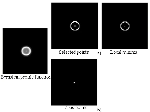
However, in the case of Bernstein profile function (Figure 11), the Gaussian profile assumption being invalid, the voxels selected using Krissian approach are located both on the axis and on the edges of the object.

Using the method introduced in this paper, only the axis voxels are selected, since no assumption regarding the profile function has been necessary. (Figure 11 b).

Results for synthetic fibers

Various cases have been considered in order to estimate the location accuracy. In the ideal case, the cylinder is taken along x, y or z, without noise. Then, the detected axis matches exactly the real axis of the cylinder.

Table 1 provides the location error, i.e. the average distance between the detected axis voxels and the real axis, in the cases of noisy profile functions and oblique axes. The Signal to Noise Ratio is SNR=20.log(S/B)), where S is the signal amplitude and B the noise amplitude. The noise is Gaussian and additive. Figure 12 shows the case of an oblique axis orientation, SNR=12dB and the error is less than 1 voxel.

3.2 Results on a fiber-reinforced composite material

The approach has also been applied to real 3-D data, obtained from a partially densified carbon/carbon (C/C) composite material [18]. This fiber-reinforced material is composed of three phases (Figure 13):

• A fibrous reinforcement made of quasi-cylindrical fibers. • A matrix (the coating used to bind the fibers).

3-D images of this material were acquired on ID19 beamline at ESRF (European Synchrotron Radiation Facility) by Synchrotron X-ray Micro Tomography (SXMT). The main characteristic of ID19 beamline is its length (145 m), which helps to obtain a strong coherent beam. The chosen resolution is 0.7µmper pixel and the number of views is 1500 projections. Due to the coherence properties of the X-ray beam and to the nature of the composite material (low absorption contrast), phase contrast tomography mode was used [19]. The characteristics of the resulting blocks are a bright / dark alternation at the borders of the components. Inside these blocks, the fibers appear as cylindrical isosurfaces centered on the fiber axis. An interesting point is that the matrix is also composed of cylindrical isosurfaces that are locally centered on the fiber axis.

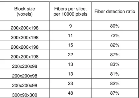
For test purposes, a data set has been built from nine 3-D extracts of various size (200x200x198 voxels, 200x200x32 voxels, 300x90x300 voxels), and for which the average density of fibers per slice varies from 9 to 48 per 10.000 pixels.

In order to suppress some detection errors due to some cylindrical porous spaces, a preliminary segmentation first eliminates small pores lying inside the bundles of fibers (Figure 14).

Table 2 shows ratio of detected fibers for this dataset. The detection ratio varies from 72% to 87%, with an average ratio of 82%.

It should be noted that, for application purpose, fibers in contact with an edge of the block are not taken into account.

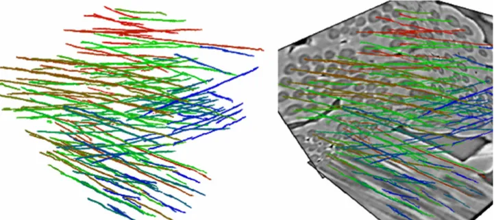
Figure 15 shows the result obtained for a block from this dataset. The average density for this block is 48 fibers per 10.000 pixels per slide and the ratio of detected fibers is 87%. For the extract shown in Figure 16, the detection ratio is 87% for an average density of 22 fibers per 10.000 pixels per slide. In Figure 17, the extract fiber density is less than 15 fibers per 10.000 pixels per slide. Moreover Figure 17 fibers show clearly two distinct directions. Nevertheless, the axes are found whatever the orientation and 82% of the fibers are detected.

For each block in the dataset, the detected axes are located closely to the actual axes of the fibers, according to expert perception. Nevertheless, even if the detection is mostly accurate, there are still two kinds of error.

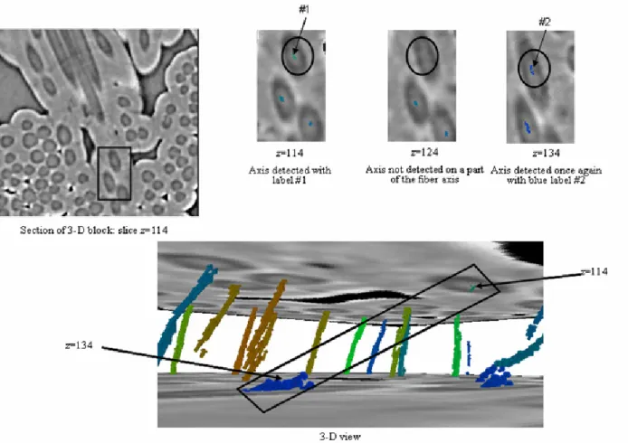
The first one is a lack of detection of the fiber axis. This occurs generally when the fiber can not be considered as cylindrical or when the limit between fibers can not be distinguished (Figure 18). The second one consists in erroneous detection of the fiber axis. In the ideal case, a fiber is detected all along the fiber axis by one axis with one label. Unfortunately, in some cases, the fiber is detected only on one part of the axis (Figure 19), or / and with two or more axes and labels (Figure 20). So some fiber axes can appear truncated. Fiber length will then be underestimated and some fibers will be counted several times. Nevertheless, these cases are infrequent, and some post processing stages can be used to complete the missing axis points and to merge coinciding axis labels for a given fiber.

4. CONCLUSION

This paper introduces a coarse-to-fine algorithm dedicated to the detection of the axes of cylindrical objects in 3-D images. The approach relies on the geometrical properties of the cylinder and uses gradient and curvature estimations.

An original gradient operator, G3D10 has been specifically designed. It provides optimized estimation of the orientation toward the axis of a cylinder in a 3-D block.

Then, the axis detection operates in a coarse-to-fine scheme. The coarse step of the approach provides a set of connected components surrounding the actual axis of the fibers. This step is based on gradient estimation obtained using G3D10. At this stage, almost all fibers are detected, but the resulting axes lack of accuracy and appear as thick connected components. The second step then consists in computing the central axis inside each connected component.

The various experiments made on both synthetic data and fiber-reinforced composite materials show that more than 80% of the fibers are detected and the axes are accurately located. Some detection errors appear, especially when the cylindrical assumption is not valid. Nevertheless, most errors can be corrected using simple post processing techniques.

Using the geometry of the detected axes, the characterization of a fibrous reinforcement becomes possible and allows obtaining valuable information such as fibers ratio in each direction, distribution of the length and radius of fibers, curvature. It can also provide useful data for physico-chemical numerical simulations. Moreover, the axis location can be used as the initial step of segmentation algorithms, such as region-growing algorithms or active contour methods.

ACKNOWLEDGEMENTS

The authors wish to thank Région Aquitaine for financial support through ARA (Aquitaine Rentrée Atmosphérique) association.

REFERENCES

[1] R. Blanc, Ch. Germain, J.P. Da Costa, P. Baylou and M. Cataldi, “Fiber orientation

measurements in composite materials”, Composites Part A, 37, 197-206 (2006)

[2] J. Lux, C. Delisée, X. Thibault, “3D characterization of wood-based fibrous materials: An application”, Image Anal Stereol, 25, 25-35 (2006)

[3] K. Krissian, G. Malandrain, N. Ayache, R. Vaillant and Y. Trousset, “Model-Based

Detection of Tubular Structures in 3D Images”, Computer Vision and Image Understanding, 80 (2), 130-171 (2000)

[4] D. Attali and A. Montanvert, “Computing and simplifying 2D and 3D continuous Skeletons”,

Computer Vision and Image Understanding, 67, 261-273 (1997)

[5] T. Rabbani and F. van den Heuvel, “Efficient Hough transform for automatic detection of

cylinders in point clouds”, Proc. The 11th Annual Conference of the Advanced School for Computing

and Imaging (ASCI’05), Het Heijderbos, Heijen, The Netherlands (2005)

[6] C.R. Brio and C.L. Fennema, “Scene analysis using regions”, Artificial Intelligence, 1 (3-4),

205-226 (1970)

[7] T.F. Chan and L.A. Vese, “Active contour and segmentation models using geometric PDE’s

for medical imaging”, Geometric Methods in Bio-Medical Image Processing, Series: Mathematics and Visualization, Springer, 63-75 (2002)

[8] M. Kas, A. Witkin and D. Terzopoulous, “Snakes-active contours models”, International

[9] M. Koller, G. Gerig, G. Székely and D. Dettwiler, “Multiscale Detection of Curvilinear Structures in 2-D and 3-D Image Data”, International Conference on Computer Vision, 864-869 (1995)

[10] C. Lorenz, I.-C. Carlsen, T.M. Buzug, C. Fassnacht and J. Weese, “Multi-scale line

segmentation with automatic estimation width; contrast and tangentiale direction in 2D and 3D medical images”, ProcCVRMed-MRCAS 1997, LNCS 1205, 233-242, (1997)

[11] Y. Sato, S. Nakajima, H. Atsumi, N. Shiraga, S. Yoshida, T. Koller, G. Gerig and R. Kikinis,

“Three-dimensional multi-scale line filter for segmentation and visualization of curvilinear structures in medical images”, Medical Image Analysis, V.2, 143-168 (1998)

[12] M. Hernandez Hoyos, A. Anwander, M. Orkisz, J.P. Roux, P. Douek and I. E. Magnin, “A Deformable Vessel Model with Single Point Initialization for Segmentation, Quantification and Visualization of Blood Vessels in 3D MRA”, Lecture Notes in Computer Science, 1935, MICCAI, 735-745 (2000)

[13] B. Verdonck, I. Bloch and H. Maître, “Accurate segmentation of blood vessels from 3D medical images”, in Proc.ICIP’96 – IEEE International Conference on Image Processing, Lausanne, 311-314 (1996)

[14] J.F. Canny, “A computational approach of edge detection”, IEEE Trans. Pattern Analysis Machine Intelligence, 8(6), pp. 679-698, (1986)

[15] C. Mulat, M. Donias, P. Baylou, G. Vignoles, Ch. Germain, “Optimal orientation estimators

for detection of cylinders axis”, Signal, Image and Video and Processing, in press, DOI: 10.1007/s11760-007-0035-2.

[16] H. Knutsson, “Representing local structure using tensors”, The 6th Scandinavian Conference

on Image Analysis, 244-251 (1989)

[17] O. Monga and S. Benayoun, "Using Partial Derivatives of 3D Images to Extract Typical Surface Features", Computer Vision and Image Understanding, 61 (2), 171-189 (1995).

[18] J. Martin-Herrero, “Hybrid object labelling in digital images”, Machine Vision & Application, 18(1):1–15, (2007)

[19] O. Coindreau and G.L. Vignoles, “Assessment of structural and transport properties in fibrous C/C composite performs as digitized by X-ray CMT. Part I: Image acquisition and geometrical properties”, Journal of Materials Research, 20, 2328-2339 (2006)

[20] G. L. Vignoles, “Image segmentation for phase-contrast hard X-ray CMT of C/C

Tables SBR Axis location ∞ 17 dB 12 dB 5 dB 3 dB Axis along z deg 45 = θ ϕ =45deg

0 voxel 0.01 voxel 0.57 voxel 1.3 voxels 1.5 voxels Oblique axis

deg 65 =

θ ϕ =65deg

0.4 voxel 0.67 voxel 0.71 voxel 1.27 voxels 2.5 voxels

Table 1: axis detection error

Block size (voxels)

Fibers per slice,

per 10000 pixels Fiber detection ratio

200x200x198 9 80% 200x200x198 11 72% 200x200x198 15 82% 200x200x198 22 87% 200x200x98 13 83% 200x200x98 13 81% 200x200x98 23 82% 300x90x300 48 87%

Figures

Figure 1: Extract of fiber-reinforced material observed at the ESRF (European Synchrotron Radiation Facility (ESRF, ID19 beam line) synchrotron X-ray micro tomography.

Figure 3: Example of mask m_x for G3D10 in 3-D case: (a) 3-D representation; (b) mask coefficients in the plane (O₁,k, j)

r r

with O₁ =(1,0,0); (c) mask coefficients in the plane (O₂,k, j) r r with ) 0 , 0 , 2 ( 2 =

O . Notes that here the coordinates of O₋₂, O₋₁,O₁and O₂are respectively (−2,0,0), ) 0 , 0 , 1

(− , (1,0,0)and (2,0,0). For a complete representation of mx, the same sections exist respectively in i=−1and i=−2 with negative coefficients.

Figure 4: Maximal angle error versus Signal to Noise Ratio (SNR) for G3D10, Prewitt, Sobel and cross masks, in a 3-D bloc showing a synthetic oblique cylinder (profile function order is n = 9); The

orientation error is computed for pixels with the axis distance r=3±0.5for various Signal to Noise Ratio. θ= 90 deg. and ϕ = 63 deg. The signal is the gradient norm. The noise is additive, white and

Figure 5: Estimation of the direction “of the axis” (ur₃) and “toward the axis” (ur₁) at voxel M

Figure 7: Setting the section of a cylinder: the most orthogonal plane to the axis vector s chosen in

yz xz xy, , .

Figure 8: Estimation of an axis point and its corresponding orientation thanks to the connected component voxels in the section defined by the most orthogonal plane to the axis vector chosen in

yz xz xy, , .

Figure 9: (a) Bernstein profile function of cylinder (synthetic fiber); (b) Result of axis detection on synthetic fiber.

Figure 10: Comparison of methods with Gaussian profile function a) Krissian approach and b) method introduced in this paper

Figure 11: Comparison of methods with Bernstein profile function a) Krissian approach and b) method introduced in this paper

Figure 13: Composite material observed at the ESRF (European Synchrotron Radiation Facility (ESRF, ID19 beam line) synchrotron X-ray micro tomography. Various phases are shown: fibers,

matrix and porous space.

Figure 14: (a) Results of axes detection without preprocessing; (b) with preprocessing. The circled area consists in a small pore inside the bundle of fibers.

Figure 15: Results of axes detection for a 3-D block extract of size 300x90x300. The fibers show the same direction.

Figure 16: Results of axes detection for a 3-D block extract of size 200x200x32

Figure 17: Results of axes detection for a 3-D block of size 200x200x198 with fibers with various orientations.