Technical progress in North and welfare gains in South under nonhomothetic preferences

HAL Id: halshs-00588310

https://halshs.archives-ouvertes.fr/halshs-00588310

Preprint submitted on 22 Apr 2011

HAL is a multi-disciplinary open access

archive for the deposit and dissemination of

sci-entific research documents, whether they are

pub-lished or not. The documents may come from

teaching and research institutions in France or

L’archive ouverte pluridisciplinaire HAL, est

destinée au dépôt et à la diffusion de documents

scientifiques de niveau recherche, publiés ou non,

émanant des établissements d’enseignement et de

recherche français ou étrangers, des laboratoires

Technical progress in North and welfare gains in South

under nonhomothetic preferences

Lilas Demmou

To cite this version:

Lilas Demmou. Technical progress in North and welfare gains in South under nonhomothetic

prefer-ences. 2007. �halshs-00588310�

WORKING PAPER N° 2007 - 08

Technical progress in North and welfare gains in South

under nonhomothetic preferences

Lilas Demmou

JEL Codes: F11, O11

Keywords: Dornbush-Fisher-Samuelson Ricardian

model, technology and trade, North-South trade,

nonhomothetic preferences, hierarchic needs,

hierarchic purchases

P

ARIS

-

JOURDAN

S

CIENCES

E

CONOMIQUES

L

ABORATOIRE D

’E

CONOMIE

A

PPLIQUÉE

-

INRA

48,BD JOURDAN –E.N.S.–75014PARIS TÉL. :33(0)143136300 – FAX :33(0)143136310

www.pse.ens.fr

Technical progress in North and welfare gains in South

under nonhomothetic preferences

Demmou Lilas

February 2007

Abstract

The paper proposes a theoretical model investigating the welfare consequences of tech-nological shocks in a Ricardian framework (a la Dornbush, Fisher and Samuelson, 1977). Contrary to existing literature, the model incorporates a nonhomothetic demand func-tion whose price and income elasticities are endogenously determined by technology. The model is applied to the case of trade between two economies with di¤erent development levels. It is shown in particular that the developing country can experience a fall in utility as a result of technical progress in the developed country. This result depends on the type of technological shock assumed (biased vs. uniform technical progress), as well as on the size of the development gap.

Keywords : Dornbush-Fisher-Samuelson Ricardian model ; Technology and Trade ; North-South Trade ; Nonhomothetic preferences ; Hierarchic needs ; Hierarchic purchases

1 Introduction

The role of nonhomothetic preferences in the analysis of trade has experienced a sharp rise in importance in the recent literature. This assumption about consumption behavior has been included in a bunch of papers dealing with di¤erent questions such as the predicted factor content of trade (Dinopoulos, Fujiwara and Shimomura (2006), Chung (2003)), the e¤ects of trade liberalization or preferential trade agreements on welfare (Stibora and de Vaal (2007), Stibora and de Vaal (2006)), the relation between income inequality and trade ‡ows (Mitra and Trinidade (2003), Kugler and Zweimüller (2002)) and the in‡uence of technological progress on the distribution of gains from trade (Matsuyama (2000)).

The reason for including nonhomothetic preferences in a trade model, despite the lower tractability of this kind of function, is that there is much evidence to show that deviation from homothetic preferences is not marginal. One illustration of this is provided by a major …nding in the empirical literature devoted to this issue: Hunter (1991) proposes a counter-factual analysis and shows that nonhomothetic preferences account for 25% of world trade. In the same line, several empirical contributions prove that income elastic-ities in trade are actually non unitary (see, for instance, Magee and Houthakker (1969), Atesoglu (1993, 1994); Bairam, Dempster (1991); Perraton (2003) and Muscatelli et al. (1994, 1995)). However, most contributions in the existing literature are based on the assumption of homothetic preferences. This raises the question of whether certain im-portant theoretical results in trade literature are robust to changes in the speci…cation of preferences.

This paper is devoted to the old question of the international distribution of welfare gains induced by technical progress. More speci…cally, I look at the relative ability of a developing country to bene…t (in terms of welfare) from the external technical progress through trade. Among the large literature devoted to this issue, the standard approach is the Ricardian framework : according to Dornbush, Fisher and Samuelson (hereafter, DFS (1977)), technical progress in one country always bene…ts the trading partner, through a terms-of-trade deterioration for the fast-growing country. This theoretical result relies on the use of a Cobb Douglas utility function yielding unitary income and price elasticities in trade. It prevails in ma jor inter-sectorial trade models such those of endogenous growth (see for instance, Grossman and Helpman, chapter 7, 1991).

I propose here a ricardian model where non unitary elasticities in trade are microfunded on the basis of non homothetic preferences1_{. This model is related to the Ricardian} inter-sectorial trade models of Matsuyama (2000)2_{. Actually, Matsuyama (2000) proposes a} nonhomothetic model which is considered as an alternative to the standard homothetic model of DFS (1977). Matsuyama models nonhomothetic preferences through a function of hierarchic desires, where agents extend the range of consumed goods when real income increases. As the quantities of each good consumed are exogenously …xed to one, the evolution of consumption can only be extensive. The common point shared by the Mat-suyama and DFS models is that they …x, a priori, the evolution of consumption patterns in the event of technical progress. In the DFS model, demand shifts towards those goods which display the greatest decrease in relative price (so as to maintain the initial distribu-tion of spending on each good). In Matsuyama’s approach, the change in demand favours the lower priority goods produced by North.

By allowing agents to choose both the quantities and the range of goods consumed, I

1_{The theoretical interpretation of non-unitary income elasticities in trade is not straightforward.}

Ac-cording to McGregor and Swales (1986, 1991) and Krugman (1989), this result is a statistical artefact resulting from a supply composition e¤ect. On the other hand, nonhomothetic preferences occupy a central position in the post-Keynesian analysis of income elasticities of trade (Thirlwall (1979), Kaldor (1970)). This debate lies outside the purposes of this paper. The choice of a nonhomothetic preference-based approach is found in some empirical studies reported in section 2.1. More details can also be found in studies which control for the supply side composition e¤ect in their estimations of export and im-port functions: Amable (1992), Fagerberg (1988), Feenstra (1994), Gagnon (2003), Funke and Runwedel (2001), Bayoumi (1999).

2_{We can also refer to the nonhomothetic intra-sectorial models of Flam-Helpman (1987) and Stockey}

propose a new framework to account for non homothetic preferences alternative to Mat-suyama (2000). The main speci…city of my approach is the link established between the price and income elasticities of external demand, and the nature of the goods in which each country is specialized. This link forwards by two transmission channels. Firstly, I consider hierarchic consumption behavior. Goods are then distinguished according to their relative degree of priority, which also determines their respective income and price elasticity values. Secondly, the technological dimension is linked to the consumption be-havior through a function of hierarchic purchases. In particular, I allow technical progress to change the relative degree of priority of each good. The intuition behind this is that technical progress, by the creation of new goods, leads to the creation of new needs, and then modi…es the perception of agents regarding their pre-existing needs. This e¤ect is formally expressed by the fact that elasticities are partially determined by technical coef-…cients of production. Hence, technical progress has a direct impact on the distribution of spending devoted to each good and on the range and quantities of goods consumed.

The aim of the paper is then to analyze the impact of technical progress on the interna-tional distribution of welfare, in a framework where hierarchic consumption, non-uniform substitution and income e¤ects are simultaneously included. Our main result is that South can be harmed by technical progress in the North. This happens if technical progress is biased toward lower priority goods and if the size of the technological gap between the two countries is large. The decrease in South’s welfare occurs despite the fact that South’s agent consumes a wider range of goods produced by North. This result derives directly from the link established between preferences and technology. It is totally at odds with results from main inter-sectorial Ricardian models, where an increase in the existing pat-tern of comparative advantages leads to increased gains from trade (DFS (1977), Krugman (1990), Matsuyama (2000)). On the contrary, our result suggests that, for less advanced countries to avoid being harmed by North’s technical progress, there exists an optimal level of development gap with their trading partners. Due to the complexity of the model, I analytically study the case of a very large development gap between North and South. I also provide simulations for the more general case.

The rest of the paper is organized as follows. In the next section, a closed-economy model and the main properties of the demand functions are presented. In the third section, these functions are incorporated into a Ricardian model of the type developed by DFS. A model of North-South trade is then obtained where the price and income elasticities of external demand are non-unitary and micro-founded. The …nal section is devoted to the analysis of the impact of North’s technical progress on South’s welfare.

2 A nonhomothetic closed-economy model

2.1 Characteristics of consumption behavior

A series of macro- and microeconomic empirical studies on demand behavior provides direct validation for the hypothesis of nonhomothetic preferences. We can notably con-sider the following evidences. Firstly, Falkinger, Zweimüller (1996) and Jackson (1984) show that a rise in income is accompanied by an extension in the range of goods con-sumed by agents. Secondly, Hunter (1991), Hunter-Markusen (1988), Jackson (1984) and Fillat-Francois (2004), test the empirical relevance of some speci…c nonhomothetic de-mand functions (respectively, Stone Geary, Almost Ideal Dede-mand System and hierarchic consumption). They verify that when their income rises, agents do not distribute this increase uniformly over all the goods they buy3_{. Finally, a corollary from the empirical} validity of the previous nonhomothetic demand functions is that sector income elasticities depend on the agent’s level of income.

3_{It should be noted that, as the Hunter (1991), Hunter-Markusen (1988) and Francois-Fillat (2004)}

studies rely on cross section data, they indirectly control for the impact of supply change composition on demand income elasticities. One can also refer to the paper by Bills and Klenow (2000), who calculate Engel’s curve by controlling for quality.

We require a demand function which is consistent with these three previous stylized facts: hierarchic consumption, non unitary income elasticities at the sectorial level, and a link between demand income elasticities and agents’ levels of income. From a theoretical point of view, our approach to preferences is then related to that of Jackson (1984) and Hunter-Markusen (1988). They use a utility function of the following type:

U =X¯ilog(qi+ °i)di (1) where qi corresponds to the quantity of go od i consumed.

This quasi-homothetic utility function can produce a linear expenditure system (LES) or a hierarchic linear expenditure system (HLES), depending on the sign of the constant terms °i. For instance, Hunter and Markusen (1988) consider negative constant terms. In this way, they account for the need to satisfy a minimum consumption of an exogenous number of sectors4_{. Subsequently, the function produces (non unitary) income and} sub-stitution e¤ects. On the contrary, Jackson (1984) assumes a positive sign for the constant terms: the utility function relies more on an endowment e¤ect, which produces hierarchic consumption of an endogenous range of consumed goods. For some goods, the non neg-ativity constraint may e¤ectively become binding. The main interest of this approach is that it allows both for extensive and intensive demand behavior5_.

We follow Jackson’s approach. In this way, we can simultaneously account for non uni-tary elasticities of demand at the sectorial level and hierarchic consumption. Nevertheless, we modify the previous utility function in three ways. Firstly, it is expressed in continuum so that we can obtain an expression for the marginal good. Secondly, the standard Cobb Douglas coe¢cient ¯_i is assumed to be equal to one. All goods in the utility function are then symmetric, except as far as the endowment e¤ect is concerned. Thirdly, we make a linear transformation by dividing the term in brackets in equation 1 by °_i: The purpose of this last transformation is to obtain a function where only consumed goods enter into the agent’s …nal utility6_{. The individual utility function at the heart of our model can} then be written: U = 1 Z 0 log(qi °i + 1)di (2)

The maximization utility program of the representative consumer can be written: M ax U s:t: 1 Z 0 piqidi = y and qi ¸ 0

where piand y correspond respectively to the price of good i and to the agent’s income. U is given by equation 2.

We can write the Khun-Tucker conditions: for i 2 K; _p1 i°i > ¸ => qi= 1 pi¸¡ °i (3) for i 2 K;= _p1 i°i < ¸ => qi= 0 (4) for i = J; 1 pJ°_J = ¸ => qi= 0 (5)

4_{One could also refer to the approaches of Markusen (1986), Matsuyama (1992) and Puga-Venables}

(1999), who apply the minimum consumption framework in a model with two sectors.

5_{Foellmi and Zweimüller (2006) propose a closed-economy model where the utility function presents}

the same characteristics.

6_{Otherwise, according to equation 1, for all goods consumed, utility is determined by ¯}

ilog(qi+ °i),

but non-consumed goods also enter into the agent’s utility through ¯ilog(°i): Our transformation removes

According to these conditions, a good will or will not be consumed depending on its value for the term pi°i. This term determines hierarchic consumption and can then be considered as an entry criterion. Ceteris paribus, the lower the value of this term, the more likely it is that the good will be consumed, and the higher the priority attached to it. Agents will consume lower priority goods only if what are perceived as more basic needs have been already satis…ed in terms of quantity (following the equation 3)7_.

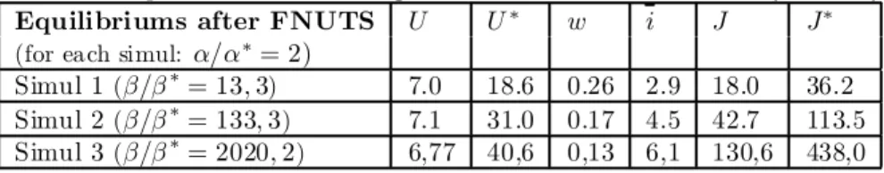
To order the consumption process explicitly and determine the marginal good J , we have to assume that the entry criterion follows an increasing monotonic function. This assumption enables us to divide the continuum into two segments: that of consumed goods i 2 K = [0; J [ and that of non-consumed goods i =2 K = [J; 1[ (…gure 1):

We can then write the Lagrange multiplier:

¸ = Z i2K di y + J R 0 pi°idi (6) Using equations 5 and 6, we can determine an implicit equation in J for the extensive demand function. Similarly, on the basis of equations 3 and 6 and simplifying by equation 7, we obtain an intensive demand function (qi):

J = y + J R 0 pi°idi pJ°J (7) piqi = pJ°J¡ pi°i if pi°i< pJ°J (8) piqi = 0 if pi°i> pJ°J

In addition, using equations 3 and 6 and deriving the induced demand function, we obtain an expression for demand income elasticity. In the same way, we can also deduce two useful expressions for own-price and cross-price elasticities.

´iy = 1 J: y piqi (9) ´i_p = ¡1 ¡ °i qi: µ 1¡1 J ¶ <¡1 ´i p = ¡1 ¡ µ_p J°J piqi ¡ 1 ¶ : µ 1¡ 1 J ¶ (10) ´ipk = 1 J: pk°k piqi > 0 (11)

We now present changes in consumption behavior according to changes in income (y) and in the ranking of the good in the continuum (i). The main properties of our demand functions are summarized by seven theorems reported in table 1. We brie‡y present the proofs for these theorems in annex 1.

From these theorems, we can highlight that in our model, the heterogeneity of agents’ consumption baskets depends partly on their levels of income, and partly on the charac-teristics of the goods supplied (if it has higher or lower priority). Changes in consumption

7_{On this point, we should explain why we have chosen to maintain sectorial di¤erences for the ° term.}

By applying the same value for °_i; the entry criterion would only depend on relative prices (i.e. on unit

values). We wanted to avoid this e¤ect, as the model refers to an inter-sectorial approach. E¤ectively, in this case, units are likely to vary from one sector to another, and there is no justi…cation for choosing

unit values as an entry criterion. The weighting with °iallows us to get around this problem. The term

°_i then refers to a pure preference e¤ect, which determines the willingness of the agent to consume a

good. In addition, multiplication by piaccounts for the possibility of consuming it according to the price

structure (given the level of income). Because of this in‡uence of price on the composition of consumption, preferences re‡ect hierachic purchases rather than hierachic desires.

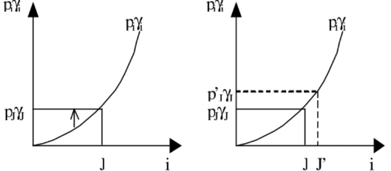
behavior resulting from an increase in income take the form of access to what had initially been non-priority (T1), together with a non uniform variation in the spending on each good (T2, T3). Based on equation 7, …gure 3 represents graphically the evolution of inten-sive and exteninten-sive consumption with income8_{. Our extensive demand function presents} also speci…c characteristics: income elasticities are in accordance with the stylized facts we aim to account for, i.e. non uniform evolution of expenditures between sectors and agents. More speci…cally, the last good to enter the consumption basket has the highest income elasticity of demand (T5). Thus, every good, except the …rst one always consumed, can be considered as a "luxury good" the …rst time it enters the agent’s consumption bas-ket. With the entry of new goods, the previously-consumed goods tend to behave more and more like necessity goods, as and when their weight in the consumption increases. Furthermore, the agents’ perceptions of the degree of priority of each good vary with their respective income levels. This is formally re‡ected by the fact that the lower the agent’s relative level of income, the more sensitive demand for good i will be to variation in income (T4).

Our extensive demand function presents two further main characteristics concerning price elasticities. As with income elasticities, a good’s level of sensitivity to price variations depends on its novelty. Agents tend to adapt their consumption in favour of the lower priority goods when there is an uniform fall in prices, and to the detriment of these same goods when there is a rise in prices (T6). These increasing values for price elasticities along the continuum seem reasonable: the higher the good’s priority, the less it is substitutable. Finally, according to the cross-price elasticity expression, the substitution e¤ect is higher than the income e¤ect. In addition, the lower the good’s priority, the more its demand is sensitive to the price variation of another good (T7).

The ranking of goods in the continuum according to their degree of priority and the pre-vious properties of our model both hold under the assumption of an increasing monotonic function for the entry criterion pi°i. The supply side of the model is de…ned such as to verify this relation. In this way, we establish a link between preferences and technol-ogy : agents’ perceptions of the priority of each good appear to be dependant on the technological dimension.

2.2 The link between technology and preferences

The supply side of the closed economy is modeled in a very simple way. We assume a single-input (labor) production function with constant returns. There are no pro…ts in the economy. Each agent’s income is then given by the wage level. The national income corresponds to total wages uniformly distributed over the population. We denote ai, the quantity of labor required to produce one unit of good i: We assume perfect competition, so that the prices of goods are given by wage (w) and the inverse of labor productivity (ai):

pi= aiw (12)

Without losing generality, we can assume that goods are ranked in the continuum in increasing order, so that the parameters of the model satisfy the following relation:

ai°i increasing function of i (13) Thus, using equation 12, pi°i is also an increasing function of i. All the properties of the consumption function described above are therefore maintained.

We should highlight the fact that the way technical progress will in‡uence equilibrium consumption derives straightforwardly from our way of modeling the hierarchic consump-tion behavior. By applying equaconsump-tion 12 and proposiconsump-tion 13 to our HLES, we e¤ectively

8_{It should be noted that the choice of a convex curve for p}

i°iis arbitrary. Theorems are valid for the

establish a link between technical progress and preferences. Technical progress, by modi-fying the values of ai°iand the entry criterion pi°i, will impact on the range of consumed goods, the share of spending devoted to each good, and their respective income and price elasticities of demand (equations 7-11). Actually, our goods ranking, which combines a technological criterion9 _(a

i) and a criterion based on the utility function (°i) ; expresses the fact that a technological shock (via ai) or a preference shock (via °i) have the same impact on the composition and evolution of consumption. This equivalence is supported by two arguments. Firstly, technical progress and increases in real income are two sides of the same phenomenon. Accordingly, every increase in income (or technical advance) involves changes in the distribution of expenditures between goods, because of Engel’s law [Pasinetti, 1983, p. 69]. Secondly, the equivalence between a technological shock and a preference shock is based on the following intuition. When a technical advance results in the creation of new goods, it also entails the creation of new needs and modi…es agents’ perceptions of pre-existing goo ds (in terms of needs)10_{. We could say that the boundary} line between "essential" needs and "psychological" needs is modi…ed1 1_.

The mechanism of an endogenous change in consumption behavior with technical progress is at the heart of our theoretical results. Technical progress, by changing real income, is likely to modify the range of consumed goods (theorem 1). But at the same time, in our model, technical progress also induces a change in the threshold level of the quantities consumed necessary to extend the range of consumption (equation 8). Variation in utility therefore depends on the evolution of these two components, quantities and range of goods consumed, which may not change in the same way. This kind of endogenous change in consumption is graphically represented in …gure 4.

At this point, it may be useful to compare our approach to preferences with that of DFS and Matsuyama. The di¤erences in demand behavior in the three models are presented in table 2. Our model is clearly distinct from DFS, where there is an homothetic demand function of the Cobb Douglas type. This exogenously constraints the range of consumed goods and the distribution of spending between goods. Nevertheless, the two models can considered close insofar as they both allow for endogenous determination of quantities consumed. Our approach also appears to be closely related to that of Matsuyama (2000), based on an utility function of hierarchic desires1 2_{. In this case, agents consume one unit} of each good according to an order of priority that is …xed a priori. As in our model, the range of consumed goods, and subsequently the share of spending devoted to each good, are endogenous. Nevertheless, his approach di¤ers from our own in that he only allows for an extensive change in consumption behavior: income and price elasticities are null for each good.

We now embed our demand function in a Ricardian trade framework. The di¤erences described above concerning the utility function of the three approaches will be re‡ected by di¤erences in the mechanisms involved in the trade balance equilibrium.

9_{Fixed capital is not explicitly introduced into the model. However, we consider that the input of labor}

represents e¤ective labor, i.e. a composite (comprising labor, capital, and human capital).

1 0_{Like Young (1991), we have not modeled the innovation of goods in our model: an in…nite number}

of goods are theoretically available for consumption, but some of them are too expensive to be produced. Technical progress makes it possible to produce these goods by reducing production costs.

1 1_{We should stress the fact that in our model, no goods, except the …rst one, can be considered essential}

in physiological terms. It is only the perception of the agents (according to income and price structure) which makes each of them relatively essential.

1 2_{The function of hierarchic desires is often used to link consumption expenditures with income}

distri-bution (Murphy, Shleifer and Vishny (1989) or Zweimüller (2000)). This is also the case in Matsuyama (2000). To be able to compare his approach with our own, we only consider the characteristics of his model under the assumption of a representative agent (i.e. with an uniform income distribution).

3 The nonhomothetic Ricardian model

3.1 International specializations and consumption

We consider two economies with di¤erent levels of development. The more developed economy is the foreign one, and it is denoted by an asterisk. The foreign wage is the numeraire (w¤_{= 1) and the domestic wage (w) then re‡ects the relative wage. The general} structure of the open-economy model is established following the standard hypotheses of DFS (1977). Firstly, it is assumed that competition in the two countries is perfect. There is therefore an international price pm

i ; which corresponds to the trade equilibrium at pmi = M infpi; p¤ig: Secondly, the foreign economy is more developed in the sense that it is more productive, in absolute terms, in every sector a¤

i < ai: Thirdly, the productivity advantage of the developed country increases along its goods continuum, i.e. ai

a¤ i is an increasing function of i.

We can demonstrate that under the hypotheses of a technological gap increasing along the whole goods continuum of the developed country, and of an identical utility function in the two countries, the ranking of goods (in terms of priority level) in the developed country entails an identical ranking in the developing country:

if @a¤i°i @i > 0 and @ai a¤_i @i > 0 then @ai°i @i > 0

In other words, the ranking of goods established for the developed economy is an "international" ranking. We can therefore identify the comparative advantage of each country in terms of the nature of goods respectively traded. Like Matsuyama (2000), we thus establish a relation between the characteristics of a country (its level of devel-opment) and the characteristics of the goods in which it specializes (relative degree of priority). Formally, the specialization equation which determines the segment of South’s specializations £0; i¤and, which holds also in the models of Matsuyama and DFS, can be written:

w =a ¤ i

a_i (14)

Given the hypothesis of the technology gap, trade can only take place if, for all i 2 £

0; i¤; p¤i > pi: For the developing country to be competitive in this goods segment, the minimum condition is that w < 1. The developing economy will then be specialized in the beginning of the goods continuum, i.e. in goods with higher priorities. These goods present a relatively lower technological gap and lower income elasticity of demand (see theorem 5)13_.

Concerning consumption, the marginal goods consumed in the two countries can be determined using equation 7:

J = w + J R 0 pm i °idi °JpmJ (15) J¤ = 1 + J_R¤ 0 pm i °idi °J¤pm_J¤ (16)

1 3_{It can be noted that this characteristic allows us to interpret the degree of priority of each good in}

terms of the degree of sophistication. Empirical studies provide evidence in favor of a positive relation between income level and the share of expenditures devoted to the importated technological, di¤erentiated, and higher quality goods (see respectively, Meliciani (2002), Francois and Kaplan (1996), Hallak (2003)).

Because agents in the two countries face identical prices for goods; the di¤erence in relative wage expresses a di¤erence in real income. We can therefore apply the main theorems de…ned in the closed economy.

Corol lary 1: The developed country consumes more products and these products are lower priority.

E¤ectively, using theorem 1 and relation 13, and given that the relative wage is less than one; we can write J¤_{> J and therefore p}m

J¤°_J¤> pm_J°_J:

According to this corollary and the previous assumptions about the technological di-mension, the structure of consumption and specializations induced by the model can be summarized as in table 314_.

3.2 Trade equilibrium

We make the standard assumption of a balance of trade equilibrium constraint where X and M represent respectively the exports of the developing country (imports of the developed country) and the imports of the developing country (exports of the developed country). On the basis of equations 8 and 12, we can write:

X = M i Z 0 pmi q¤iL¤di = J Z i pmi qiLdi iL¤a¤J¤°_J¤¡ wL¤ i Z 0 ai°idi = (J¡ i)La¤J°J¡ L J Z i a¤i°idi

Re-writing the last term (of the right hand side) using equation 15, we obtain, after simpli…cation: w = i £ L¤_a¤ J¤°J¤+ La ¤ J°J ¤ L + (L + L¤₎Ri 0 ai°idi (17)

We have …nally obtained a system of four equations (14-17) with four unknowns, which must satisfy the following conditions: 0 < i < J < J¤_:

Concerning the last expression, it should be noted that it is no easy task analyzing this trade balance equation, as it includes many endogenous variables (w; i;J; J¤_). Neverthe-less, we can make some comments on the partial e¤ects of the entry criterion terms (ai°i), that which will highlight the potential impact of technical progress on trade equilibrium. Firstly, in the numerator, a¤

J¤°J¤ and a

¤

J°J; refer to the threshold value of the marginal consumed good in each country. According to equation 8, the spending on each good is positively related to these terms. At the same time, according to equations 15-16, the range of consumed goods in each country decreases with these terms. Thus, a decrease in these boundary terms (through North’s technical progress) is likely to hurt South’s relative wage by lowering the spending devoted on its goods. On the contrary, a decrease in the integral value in the denominator re‡ects an higher gap between the threshold value of the marginal consumed good (a¤

J¤°J¤; a¤_J°_J), and the threshold value of South’s products (ai°i). This is likely to result in higher spending on each of South’s products (equation 8), and then in an increase in the relative wage.

1 4_{Concerning the structure of trade, we can also note that North is specialized in a wider range of}

products. This characteristic comes directly from theorem 2 and 3 applied to the trade balance condition. It is in accordance with some recent empirical studies which highlight the fact that high income per capita countries export a wider range of products. See, in particular, Hummels and Klenow’s paper (2005).

At this point, it is again worthy to compare the mechanisms involved in the adjustment of our trade balance equilibrium with those of Matsuyama and DFS. Looking at table 4, the di¤erences between the three models are straightforward15_{. In DFS, the trade balance} equilibrium does not depend on technical coe¢cients. This is due to the Cobb Douglas function, according to which the share of spending on each good is …xed by the parameter ¯_i. Every technical progress will have the e¤ect of increasing the quantity demanded in proportion to the fall in price. In Matsuyama, the trade balance equilibrium no longer depends on the relative wage, but only on South’s technical coe¢cients. This comes from the use of the function of hierarchic desires, where the quantities demanded are constrained to one. As North is specialized in lower priority goods, this entails that agents in the two countries only use their increase in real income to demand goods produced by North. It follows that demand for South’s products is insensitive to price variation, and hence to wage variation. The only way to modify external demand for South is through its own technical progress, enabling it to extend its range of specializations. In other words, under a function of hierarchic desires and an uniform distribution of income within each country, di¤erences in income elasticities in trade are "apparent". They are determined by the relative ability of each country to extend its range of traded goods16_{. North is} in this case more favored, as every change in real income is used to demand its (lower priority) goods. Contrary to our approach, non unitary income elasticities in trade, in Matsuyama’s model, are then not founded on the characteristics of the good itself, but on the assumption of an unconditional preference for North’s goods. This distinction between the two models is at the heart of the di¤erences in the trade balance equations.

Finally, one should insist on the fact that the simultaneous inclusion of extensive and intensive consumption di¤erentiates strongly our model from these two approaches. Rel-ative wage is still a determinant of our trade balance equilibrium, because of demand sensitivity to price variation. Moreover, the inclusion of both countries’ technical coef-…cients in the trade balance equilibrium accounts for our endogenous elasticities. This re‡ects the impact of every technical progress on the share of spending devoted to each country.

We now turn to the implication of our approach for the analysis of the international di¤usion of welfare gains through trade. According to the above comparisons, we have decided to devote a particular intention to the impact (on South’s welfare) of a North’s technical progress biased toward the less priority goods in the case of a large technological gap. E¤ectively, we expect speci…c results in that con…guration at least for two reasons. Firstly, in our model, the size of the technological gap between the two countries will have a direct in‡uence on the value of trade elasticities, as the latter depends on the level of income of the agents. Secondly, the nature of the technical progress is also expected to be crucial because a good’s demand elasticity depends directly on its technical coe¢cient of production. The analytical study of this case is conduced under speci…c functional forms and completed by simulations.

4 The e¤ect of a North’s technical progress on South’s

welfare

4.1 The critical in‡uence of the size of the technological gap and

the nature of the technical progress

The choice of a functional form for a Ricardian inter-sectorial trade framework is not a trivial issue. In the standard interpretation of Dornbush, Fisher and Samuelson (1977), the

1 5_{The main equations of the models of Matsuyama and DFS are presented in annex 3a.}

1 6_{Following Krugman (1989), these aggregate elasticities of external demand can be viewed as}

"appar-ent" because they do not refer to the evolution of demand for a given consumption basket, but to the changes in the composition of traded goods.

continuum of goods involves di¤erent sectors, the characteristics of which are not de…ned. The only precision made concerning sector characteristics is a ranking of goods along the continuum as a function of the relative productivity gap between the two countries. Krugman (1990) proposed an extension of the theoretical interpretation that can be made of the DFS model: he argued that the ranking of goods according to the productivity gap corresponds to the ranking of goods according to their technological content. However, choosing a functional form which can take into account the link between technological content and sector productivity is no easy task, insofar as that if the continuum involves di¤erent sectors, the respective units of each good are likely to be di¤erent. In other words, it is impossible directly to establish the relation between aiand i. In our model, we get around this problem by not directly …xing the functional form of ai; but only that of ai°i; which we have de…ned as an increasing function of i (relation 13):In other words, we do not …x the primitives of the expressions for ai°i and a¤i°i. We propose to use the following functional forms:

ai°i = ® + ¯:i (18) a¤i°i = ®¤+ ¯¤:i (19) In addition, our hypotheses about the technological gap will enable us to constrain parameter values. For an absolute productivity advantage increasing along the continuum, the su¢cient condition to allow South to be competitive in the …rst part of the continuum is:

¯ ¯¤ >

® ®¤ > 1 In this case, the ratio of production costs (a¤i

ai) decreases along the whole continuum with an asymptote tending to ¯¤

¯:

We rewrite the general equilibrium model by applying the equations 18-19 to the system 14-17 and verify that an analytical solution exists17_{. We then analyze the e¤ect} on South’s utility of a biased technical progress (toward the less priority goods) in North when the technological gap is large This con…guration is formally equivalent to a decrease in the value of ¯¤ _{when this parameter is very small (relatively to ¯). To simplify the} analysis, we study trade equilibrium around ¯¤_{= 0:}

To do this, we denote " =p¯¤ and proceed to marginal developments of our equilib-rium equations around " = 0: Results are the following ones :

i = ei(1¡ a:") (20) w = w:(1 + b:")e (21) J = ej ":(1 + c:") (22) J¤ = ej¤ ":(1¡ d:") (23) ei; ew; ej; ej¤; a; b; c and d are all positive parameters obtained after marginal development of equilibrium equations (their expressions are reported in annex 2c).

By including (20-23) in equation 2 we obtain an expression for South’s utility. With the same methodology (marginal developments), we can demonstrate that South’s utility can be represented, around " = 0; by an equation of the following form :

U = A + B:" (24)

where :

A = ® ¯: log ® (® + ¯ei)+ ei + l (1 + l): 1 (® + ¯ei) B = 1 (® + ¯ei):®¤_{: (1 + l)}: à ej¤_{¡ ej} 1 + l + ej 3 !

In …gure 5, we have represented for speci…c value of parameters the equation 24 as well as the general utility equation (2). This con…rms that equation (24) is good approximation of our utility function around " = 0:

The two terms A and B are positive ( ej¤ _{> ej): This implies that the utility of the} developing country is an increasing function of the term " = p¯¤: Hence, the result of this analysis is that when the size of the technological gap increases (when " tends toward 0), the utility of the developing country decreases.

As a …rst comment, it is worthy to compare this result with those obtained by Mat-suyama (2000) and DFS (1977) under the same con…guration. In their model, the following Ricardian property is always veri…ed: as trade gains are derived from the existence of dif-ferences between countries, when these di¤erences grow larger, i.e. when technological shocks augment the existing terms of comparative advantage, the transaction gains in-crease1 8_{. In other words, a biased technical progress in North improves South’s welfare.} Actually, the di¤erence between these both approaches and our own model can be ex-plained on the basis of equation 20. E¤ectively, looking at equations 20-23, one can note that around " = 0; if the impact of ¯¤_{on w and on J; J}¤_{is standard (respectively positive} and negative), this is no more the case for i: The equation 20 implies that, the range of South’s specialization is negatively related with the cost of production of North. Before discussing in more details the mechanisms at the heart of this "non standard" relation-ship, we aim to complete our analysis by looking for what happens outside the previous con…guration. We proceed by simulations and relax …rst, the assumption of a very large technological gap, and second that of a biased technical progress.

For our simulations, we consider three di¤erent equilibriums, in order to measure the extent to which the qualitative results produced by the simulations are sensitive to the size of technological gap (simul 1, 2 and 3). These con…gurations di¤er in the value given to the parameter ¯¤_{. Table 5 presents the values taken by the di¤erent variables for these three} initial equilibriums. We adopt a comparative static procedure and then study South’s utility in the case of a foreign technical progress biased towards the most sophisticated goods (FNUTS, variation of ¯¤_{), and in the case of a foreign uniform technical shock} (FUTS, identical variation in ®¤_{; ¯}¤_{). These technological shocks are formally re‡ected} by a reduction in the parameters concerned by one half.

Simulations results con…rm that the size and the nature of the shock are two conditions for the appearance of a con…guration where South’s utility decreases as a result of a technical progress in North. E¤ectively, by comparing tables 5 and 6, we can see that even in the case of a very large technological gap, the South always bene…ts from North’s technical progress when the latter is uniform along the continuum. Also, in the case of a technical progress in the developed country growing over £i; J¤¤_{; the utility of the} developing country fall only under a large technological gap. This con…guration appears for simul 2 and 3 (compare tables 5 and 7). The existence of a threshold e¤ect after which the developing country may present a decrease of its utility appears clearly in …gure 6.

We now turn to the description of the main mechanisms embedded in our model which are at the heart of the process of immeserizing in South after a technical progress in North.

1 8_{Result of Matsuyama and DFS can directly be derived from their conditions of specialization (equation}

14) and their trade balance equilibrium (table 3). We have also reported graphically the impact of technical shock in …gures of annex 3b.

4.2 Mechanisms at the heart of an immeserizing e¤ect of external

growth

It is worthy to begin by an explanation of our results in the case of an uniform technical progress in the North. According to our simulations, in this con…guration, the classical e¤ect of welfare gain di¤usion holds, whatever the size of the technological gap. This can be explained in the following way. Given uniform technical progress in the developed country, the productivity gap between the two countries increases uniformly. According to the specialization equation (14), this entails a fall in the relative wage. But this fall stimulates demand for goods produced by the developing country, limiting the deterio-ration in its terms of trade. At the new equilibrium, the fall in the relative wage does not completely o¤set the initial productivity gains (…gures 7). Welfare increases in both countries. It can be noted that this result tallies with that of DFS, but di¤ers from that of Matsuyama, where the developing country is totally impervious to the developed coun-try’s technical progress. The comparison between our result and that of Matsuyama is particularly interesting. This highlights the fact that, despite unfavorable elasticities in trade, trade remains a good way to bene…t from external technical progress, once we have allowed South to bene…t from price competitiveness.

Concerning now the di¤erences implied by a biased technical progress, the decrease in South’s utility can be explained in the following way. Our modeling of preferences entails that the development gap (the di¤erence in per capita income) determines the di¤erences in income and price elasticities between the two countries. We can make two observations about this e¤ect. Firstly, in a similar fashion to the uniform shock described above, the developing country is relatively penalized by its elasticities in trade. Secondly, according to theorem 6, we have seen that in our model, price elasticities increase along the continuum. Under a shock biased towards the lower priority goods, the goods which bene…t from the highest price elasticities are then those which bene…t from the largest falls in price. The price elasticity and income elasticity e¤ects contribute jointly to a pronounced change in the distribution of expenditures in favor of the goods produced by the developed country. The balance of trade equilibrium condition therefore requires a fall in the relative wage, such that the developing country may see a fall in its aggregate real income. As can be seen in …gures 8, the real costs of some consumed goods for the developing country have risen. More precisely, the adverse impact of North’s biased technical progress appears to be conduced by two e¤ects. Firstly, some goods which were previously produced by North are now produced by South, and consumed with higher real prices. Secondly, the fall in the relative wage reduces South’s purchasing power for some of North’s goods. Actually, South does not bene…t from an reinforcement of the existing terms of comparative advantage, because the strong change in the spending patterns forces South to extend its specializations, despite the reduction in its comparative advantages (see tables 5 and 7; equation 22). The wider the development gap between the two countries, the more this extension, necessary to return to the trade balance equilibrium, will penalize the developing country in terms of changes in purchasing power. One should also insist on another characteristic of our model : technical progress hurts the South despite the fact that South’s agents ultimately consume more sophisti-cated goods at lower prices (J increases). This result di¤ers strongly from Matsuyama’s approach, where J can be viewed as a direct measure of utility. In our model, changes in agents’ utilities have to be apprehended through changes in the quantities and range of goods consumed. What happens here is that the increase in utility induced by a wider range of consumed goods is o¤set by lower quantities of each good consumed. With this kind of shock, there is actually a stronger change in the slope of the curve pi°i

w ; compared with the changes entailed by an uniform shock (see …gures 7 and 8). This change re‡ects the strong modi…cation in the consumption behavior of the agents, especially in their per-ception of the relative priority of each good. With a ‡atter curve, agents view goods that had been previously considered as lower priority goods, as now having relatively more priority. They extend the range of consumed goods accordingly. At the same time, the

spending on relatively higher priority goods decreases (equation 8). This means that the fall in real income results in a reduction in the level of satisfaction provided by each good. In other words, in our model, changes in price structure indirectly account for changes in what we can call the "standard of consumption": South’s agents import a wider range of sophisticated goods (for instance, televisions or cell phones), to the detriment of the quantities of each good consumed (housing, clothes, etc.)19_.

Finally, it is worthy to brie‡y explain the reasons for which this con…guration doesn’t appear in the approaches of Matsuyama (2000) and DFS (1977). The di¤erence with our own model comes from the fact that, according to their assumption on preferences, in both other models the range of specialization does not increase as a result of this kind of shock. Notably, as it has been already noted, in Matsuyama’s model the trade balance condition is not modi…ed by biased foreign technical progress. Consequently, the range of South’s specializations remains constant. The fall in the relative wage is directly determined in equation 14 by the decrease in productivity of the marginal good i: As the productivity gains are increasing along £i; J¤¤_{; this implies that South’s consumers} bene…t from an increase in their purchasing power for all goods after i. In the DFS model, North’s technical progress is accompanied by a reduction in South’s specializations. South’s consumers bene…t from an increase in welfare through the increasing purchasing power gains along the goods continuum.

To conclude, the endogenous change in consumption and specialization in our model can be interpreted from the perspective of the product cycle theory20_{. The biased technical} progress in North has two main e¤ects on specializations. On the one hand, it stimulates North’s production of sophisticated products, and on the other hand, it induces North to give up the production of less sophisticated goods (which are being produced by South). South’s access to more sophisticated goods increases, because of the standardization of North’s production. At the same time, South becomes more competitive in some products, because of the increase in its relative poverty.

5 CONCLUSION

This paper proposes a new framework for analyzing the changes in South’s welfare induced by domestic and external technical progress. Our main contribution concerns the way we model consumption behavior. We have considered a hierarchic linear expenditure system. Goods can then be distinguished according to their order of entry into the consumption basket. This determines their relative degree of priority, and their respective income and price elasticity values. Moreover, we have established a link between these goods’ characteristics and the technological dimension. In this way, agents’ perceptions of the relative priority of goods are dependent on the type of technical progress. We have compared our results with those of Matsuyama (2000) and DFS (1977). As in our model, Matsuyama establishes a connection between technical progress, its income e¤ect, and the change in spending patterns due to nonhomothetic preferences. This also highlights the di¤erential impact of technical progress on welfare, depending on specialization patterns.

1 9_{Some vertically di¤erentiated models also produce a con…guration where North’s technical progress}

may be immiserizing for South. Nevertheless, the mechanisms involved are di¤erent. For instance, Stockey (1991) assumes a model where vertically di¤erentiated goods are imperfect substitutes. North’s agents then consume a wider range of quality goods. She shows that external progress is immiserizing for South, if it is biased toward non-traded goods (i.e. high quality goods consumed only by North). In our model, this con…guration appears even if the technical progress bene…ts traded goods. Flam and Helpam (1987), consider a model with heterogenous population in each country. South (North) produces a low (high) quality good consumed by poor agents in the two countries. In this case, the global distribution of spending is dependant on the distribution of income. If the distribution of income shifts toward the agents who consume high quality goods, this entails a change of spending patterns in favor of North. The subsequent improvement in its terms of trade may be immiserizing for South. In our model, South can lose even under our assumption of a representative agent.

2 0_{See for instance, the three stages of product developement in Vernon (1966, 1979), the models of}

Grossman and Helpman (1991), and the empirical studies of Schoot (2004), Feenstra-Rose (2000), and Hummels-Klenow (2005).

The main contribution of our model, compared with that of Matsuyama, involves our endogenous demand for quantities (and the subsequent endogenous income and price elasticities). By giving up the constraint of the (0,1) consumption framework, we bring new insights concerning the mechanisms at the heart of evolutions in welfare. More speci…cally, technical progress, by changing price structure, also modi…es the relative priority of goods. This e¤ect is notably re‡ected by a change in the level of spending (devoted to each good), necessary to extend the range of consumption. We have called this e¤ect the endogenous change in the "standard of consumption". We have shown that our model can present results that are a priori paradoxical in a Ricardian context: when there is technical progress in North biased towards the most technological goods, the greater the di¤erence between the two countries, the less the developing country gains from trade. Technical progress in North may then be immeserizing for South. This implies that there exists a level of development gap which maximize the welfare gains from trade. This result can be viewed as the re‡ection of an adverse impact of a product cycle mechanism, which is driven by consumption behavior.

BIBLIOGRAPHY

AMABLE B. (1992), E¤ets d’apprentissage, competitivité hors-prix et croissance cu-mulative, Economie Appliquée, tome XLV, n±_3.

ATESOGLU H.S. (1994), An application of the kaldorian export-led model of growth to the United States, Applied Economics, 26(5).

ATESOGLU H.S. (1993), Exports, Capital Flows, relative prices and Economic Growth in Canada, Journal of Post Keynesian Economics, 16.

BAIRAM E.I and DEMPSTER G.J. (1991), The Harrod Foreign Trade Multiplier and Economic Growth in Asian Countries, Applied Economics, 23(11).

BAYOUMI T. (1999), "Estimating Trade Equations from Aggregate Bilateral Data", IMF working paper, No. 99/74

BERGSTRAND J.H. (1990), The Hecksher-Ohlin Samuelson Mo del, The Linder Hy-pothesis and the Determinants of Bilateral Intra-Industry Trade, The Economic Journal, vol.100.

BHAGWATI J. (1958), Immiserizing growth: a geometrical note, Review of Economic Studies, 25.

BILLS M. and KLENOW P.J. (2000),Quantifying Quality Growth, NBER Working-Paper Series, n±₇₆₉₅

CHUNG C. (2003), Non homothetic Preferences as a cause of Missing Trade and Other Mysteries, working paper Georgia Institute of Technology

DAVIS D.R. et WEINSTEIN D.E. [2001], An account of Global Factor Trade, Amer-ican Economic Review, 95( 5)

DINOPOULOS E., FIJIWARA K. and SHIMOMURA K. (2006), International trade patterns under quasi-linear preferences, working paper university of Florida

DORNBUSCH, S. FISHER and P.A. SAMUELSON (1977), Comparative Advantage, Trade, and Payments in a Ricardian Model with a continuum of Goods, American Eco-nomic Review, 67(5).

FAGERBERG J. (1988), International Competitiveness, Economic Journal, 98(391). FALKINGER J. and ZWEIMÜLLER J. (1996), The Cross-Country Engel Curve for Product Diversi…cation, Structural Change and Economic Dynamics, vol.7.

FEENSTRA R.C. (1994), "New Product Varieties and the Measurement of Interna-tional Prices", The American Economic Review, vol.84.

FEENSTRA R.C. et A. ROSE (2000), "Putting Things in Order : Trade Dynamics and Product Cycles", Review of Economics and Statistics, MIT Press, vol.82(3).

FILLAT C. and FRANCOIS J.F. (2004), "National and International Income Disper-sion and Aggregate Expenditures", Tinbergen Institute discusDisper-sion paper n.04-093/2.

FLAM H. and HELPMAN E. (1987), Vertical product di¤erentiation and North-South trade, American Economic Review, 77

FOELLMI R.and ZWEIMULLER J. (2006) "Income Distribution and Demand-Induced Innovations," Review of Economic Studies, vol. 73(4)

FRANCOIS J.F. and KAPLAN S. (1996), Agregate Demand Shifts, Income distribu-tion and the Linder Hypothesis, The Review of Economics and Statistics, 78(2).

FUNKE M. and RUHNWEDEL R. (2001), "Export variety and export performance : empirical evidence from Easr Asia", Journal of Asian Economics, vol.12

GAGNON J.E. (2003), "Long-Run Supply and the Elasticities Approach to trade", International Finance Discussion papers, Board of Governors of the Federal Reserve Sys-tem

GROSSMAN G.M. and HELPMAN E. (1991), Innovation and Growth, Massachusetts Institute of Technology Press, Cambridge.

HALLAK J.C. (2003), "Product Quality and the Direction of Trade”, Journal of International Economics, (2006), 68(1)].

HOUTHAKKER H.S. and MAGEE S.P. (1969), Income and Price Elasticities in World Trade, The Review of Economics and Statistics, 51(2).

HUMMELS D.L. et P.J. KLENOW [2005], The Variety and Quality of Nation’s Trade, American Economic Review, 95

HUNTER L. (1991), "The contribution of nonhomothetic preferences to trade," Jour-nal of InternatioJour-nal Economics, vol. 30(3-4)

HUNTER L. and MARKUSEN J. (1988), Per Capita Income a Determinant of Trade, in R.Feenstra, ed. Empirical Methods and International Trade, MIT Press, Cambridge,Mass.

JACKSON L.F (1984), Hierarchic Demand and the Engel Curve for Variety, The Review of Economics and Statistics, 66(1).

KALDOR N. (1970), The Case for Regional Policies, Scottish Journal of Political Economy, nov.

KRUGMAN P.R. (1990), A "Technology Gap" Model of International Trade, in Re-thinking International Trade, MIT Press, Cambridge.

KRUGMAN P.R. (1989), Di¤erences in income elasticities and trends in real exchange rates, European Economic Review, 33.

KUGLER M. and ZWEIMULLER J. (2002), International Trade when Inequality Determines Agregate Demand, working paper 24, University of Southampton 23

MARKUSEN J.R. (1986), Explaining the Volume of Trade: An Ecletic Approach, American Economic Review, 76(5).

MARKUSEN J. and HUNTER L. (1988), Per capita Income as a basis for Trade, in Empirical Methods for International Trade, ed. R.C. Feenstra, Cambridge, MA MIT Press.

MATSUYAMA K. (2000), A Ricardian Model with a Continuum of Goods under Non-homothetic Preferences: Demand Complementarities, Income Distribution, and North-South Trade, Journal of Political Economy, 108

MATSUYAMA K. (1992), Agricultural Productivity, Comparative Advantage and Economic Growth, Journal of Economic Theory, 58.

MITRA D., TRINDADE V., (2005), Inequality and trade, Canadian Journal of Eco-nomics, Vol. 38, No. 4, pp. 1253-1271

Mc GREGOR P.G. and SWALES J.K. (1991), Thirwall’s Law and balance of payments constrained growth: further comment on the debate, Applied Economics, 23.

Mc GREGOR P.G. and SWALES J.K. (1986), Balance of payments constrained growth: a rejoinder to Professor Thirlwall, Applied Economics, 18.

MELICIANI V. (2002), The Impact of technological specialisation on national perfor-mance in a balance-of-payments-constrained growth model, Structural Change and Eco-nomic Dynamics, 13(1).

MURPHY K.M., SHLEIFER A. and VISHNY R.(1989), Income Distribution, Market Size, and Industrialization, The Quaterly Journal of Economics, August.

MUSCATELLI V., T.G. SRINIVASAN et D. VINES (1994), The empirical Modelling of NIE exports : an evaluation of di¤erent approaches, Journal of Development Studies, 30.

MUSCATELLI V., A. STEVENSON et C. MONTAGNA (1995), Modeling agregate manufactured exports for some Asian newly industrialized economies, Review of Eco-nomics and Statistics, 77.

PASINETTI L. (1981), Structural Change and Economic Growth, Cambridge Univer-sity Press.

PUGA D., VENABLES A.J. (1999), Agglomeration and economic development : Im-port substitution vs. trade liberalisation, Economic Journal, 109

PERRATON J. (2003), Balance of Payments Constrained Growth and Developing Countries: an examination of Thirlwall’s hypothesis, International Review of Applied Economics, vol.17.

SCHOTT P.K. [2004], Across-Product versus Within-Product specialization in Inter-national Trade, Quaterly Journal of Economics, 119(2).

STIBORA J. and de VAAL A. (2006), Does Preferential Trade Bene…t Poor Countries? A General Equilibrium Assessment with Nonhomothetic Preferences, working paper

STIBORA J. and de VAAL A. ,(2007), Trade Policy in a Ricardian Model with a Continuum of Goods under Nonhomothetic Preferences, forthcoming. in Journal of De-velopment Economics,

STOKEY N.L. (1991), The Volume and the Composition of Trade Between Rich and Poor Countries, Review of Economic Studies, 58.

THIRLWALL A.P. (1979), The Balance of Payments Constraint as an Explanation of International Growth Rate Di¤erences, Banca Nazionale del Lavoro Quaterly Review, 32(128).

TREFLER D.[1995], The Case of Missing Trade and Others Mysteries, American Economic Review, 85(5).

VERNON R. (1966), International Investment and International Trade in the Product Cycle, Quaterly Journal of Economics, 80.

YOUNG A. (1991), Learning by Doing and the Dynamic E¤ects of International Trade, The Quaterly Journal of Economics, may.

ZWEIMÜLLER J. (2000), Schumpeterian Entrepreneurs Meet Engel’s Law: The Im-pact of Inequality on Innovation-Driven Growth, Journal of Economic Growth, 5(2). 24

TABLES

Table 1: Main characteristics of our demand function

Income variation (y) Rank of good variation (i) Range of products @J @y > 0 T1 Share of spending @piqi @y > 0 T2 @piqi @ i < 0 T3 Income elasticities @´iy @y < 0 T4 @´i_y @i > 0 T5 Price elasticities @j´ipj @ i > 0 T6 Cross-price elasticities @´ipk @ i > 0 T7 Table 2: Main properties of the demand function of the three models

DFS (1977)

C obb D o uglas H ierarchic des iresMats (2000) Hiera rchic purchasesCurrent model ´i y = 1 0 ´iy(y; i) ´i p = 1 0 ´ip(y; i) J = J¤_{= cst J(y; p) J (y; p)} qi= qi(y; p) 1 qi(y; p) piqi y = ¯i= cst piyqi(J; p) piqi y (J; qi; p)

Table 3: Structure of consumption and specializations in the two countries

Specializations_£ Price Country of production Country of consumption 0; i¤ wai Developing country Both countries £

i; J¤ a¤i Developed country Both countries [J; J¤_{] a}¤

i Developed country Developed country Table 4: Trade balance equilibrium conditions

DFS (1977) Matsuyama (2000) wL 1 R i ¯i= L¤ i R 0 ¯i L = (L + L¤) i R 0 aidi

Table 5: Initial equilibriums according the technological gap Initial equilibriums U U¤ w i J J¤

(for each simul: ®=®¤= 2)

Simul 1(¯=¯¤= 6; 7) 6,7 15,0 0,31 2,6 14,2 25,7 Simul 2(¯=¯¤= 66; 7) 7,2 27,4 0,19 4,0 32,7 80,5 Simul 3(¯=¯¤= 1010; 1) 6.8 38.9 0.14 5.8 97.0 310.2 [® = 0:045; ®¤ _{= 0:0225; ¯ = 0:020; L = L}¤_{= 1]}

Table 6: Equilibriums after foreign uniform technical shock (FUTS) Equilibriums after FUTS U U¤ _{w i J J}¤ (for each simul: ®=®¤_{= 4)}

Simul 1(¯=¯¤= 13; 3) 6.9 23.6 0.16 2.1 14.6 36.4 Simul 2(¯=¯¤= 133; 3) 7.5 46.5 0.10 3.5 34.6 114.8 Simul 3(¯=¯¤= 2020; 2) 7.0 72,0 0,07 5,5 101,7 444,5 Table 7: Equilibriums after foreign non uniform technical shock (FNUTS)

Equilibriums after FNUTS U U¤ _{w i J J}¤ (for each simul: ®=®¤_{= 2)}

Simul 1(¯=¯¤= 13; 3) 7.0 18.6 0.26 2.9 18.0 36.2 Simul 2(¯=¯¤= 133; 3) 7.1 31.0 0.17 4.5 42.7 113.5 Simul 3(¯=¯¤= 2020; 2) 6,77 40,6 0,13 6,1 130,6 438,0

FIGURES

Figure 1: Range of consumed goods according to the entry criterion ( 1 pi°i)

1/(p

_γ

)

λ

J

(0; J) represent the segment of consumed goods under the assumption of a decreasing monotonic function for 1

pi°i

Figure 2: Proof of theorem 1:The number of consumed goods J is an increasing function of y

J

p

γ

p

γ

p

γ

y

∫

p

γ

di

As y increases, the area of the triangle above the curve pi°i increases, which is expressed by an increase of consumed goods:

Figure 3: The change of the quantities and varieties consumed with income variation

p

γ

p

γ

J J’

i

p

γ

p’

γ

p

γ

p

γ

J

i

p

γ

Along the continuum, the distance between pJ°J and pi°i indicates the spending devoted to each good.

Figure 4: The impact of prices change on the composition of consumption

p

γ

p ’

γ

p

γ

J

J ’

i

p

γ

p ’

γ

Figures 5: South’s utility

The general function (equation 2) is represented by the normal line and the border case (around " = 0) by the doted line (equation 24).

Figure 6: Utility in developing country and technological gap

6,4 6,6 6,8 7,0 7,2 7,4 7 19 55 157 451

The vertical axis represents the utility of developing country and the horizontal axis reports the value taken by ¯=¯¤_{(under the asumptions ®=®}¤ _{= 2 and constant)}

Figures 7: E¤ect of FUTS on real prices of goods (pm_i w)consumed by devel-oping country21 FUTS / Simul 1 FUTS / Simul 2 FUTS / Simul 3

2 1_{The horizontal axis corresponds to the continuum of goods (i). The normal line represents the real}

price of consumed goods in South before the shock. The doted line represents the real price of these goods after the shock. The break in the lines refers to i:

Figures 8: E¤ect of FNUTS on real prices of goods (pm_i w) consumed by developing country FNUTS / Simul 1 FNUTS / Simul 2 FNUTS / Simul 3

ANNEXES

ANNEX 1: Demonstrations of seven theorems on consumption Theorem 1: The number of goods consumed J is an increasing function of y

This can be demonstrated graphically using equation 7 (…gure 2). When y increases, the number of goods consumed J increases, as does its threshold value pJ°_J: This is expressed by the increase in the area of the triangle above the curve pi°_i: For given prices of goods, the values of variables pJ°_J and J therefore represent a wealth e¤ect.

Theorem 2: The amount spent on each good piqi is an increasing function of y This is proved simply by applying theorem 1 in equation 8: as J and therefore pJ°_J are an increasing function of y, it follows that the amount spent on each good piqi is also an increasing function of y:

Theorem 3: The amount spent on each good piqi is a decreasing function of i This can also be demonstrated on the basis of equation 8, according to which, the amount spent on a good piqiis given by the gap between the threshold e¤ect value of the marginal good and the threshold e¤ect value of the good i. The amount spent on each good is therefore a decreasing function of that good’s position in the continuum:

Theorem 4: Income elasticity ´i

y is a decreasing function of y

This is proved by using equation 9 to calculate the expression pk°k of good k which satis…es the condition ´k

y = 1: To prove this theorem, it is then su¢cient to verify that when income increases, this good corresponds to a higher index value in the continuum, @pk°k=@y > 0. Given that income elasticities increase along the continuum (theorem 5), we denote k (´k

y= 1) the good which marks the limit between the "luxury goods" segment (´i

y> 1) and the "necessity goods" segment (´jy< 1). Using equations 8 and 9, and after transformation (using equation 7), we can write for this good:

pk°k = J R 0 pi°idi J (25)

To prove theorem 4, we must verify that when income increases, the good k (which satis…es the condition ´k

y = 1) corresponds to a higher index value in the continuum of goods(@(pk°k)

@ y > 0). Using partial derivative, one can …rst deduce from theorem 1 that @J

@y > 0: Second, it is straightforward to show that when we calculate the partial derivative according to J and simplify the result (using equation 7), we obtain:

@(pk°k) @J =

y J2 > 0 Theorem 5: Income elasticity ´i

y is an increasing function of i This theorem is directly proved by applying theorem 3 to equation 9. Theorem 6: The absolute value of price elasticity ¯¯´i

p ¯

¯ is an increasing function of i This can be directly derived from the application of theorem 3 to equation 10. Theorem 7: The substitution e¤ect is an increasing function of i (for a given change in the price of a good k)

This is proved directly by applying theorem 3 to equation 11. ANNEX 2a: New equilibrium conditions

w = ®¤+ ¯ ¤_:i ® + ¯:i (26) J2_{= i}2₊ w ¯¤(2¡ ¯i 2 ) (27) J¤2= i2+ (2¡ w¯ i 2 ) ¯¤ (28)

Consequently, it is indeed veri…ed that J¤_{> J when w < 1:}

On the basis of these three equations, we can determine a polynomial for i: P (i) = ®¤ à l¡ (1 + l)¯i 2 2 ! +¯¤i µ l + (1 + l)i(® +¯i 2)¡ ¡ ® + ¯i¢(J¤_{+ lJ )} ¶ (29) = 0 With l = L L¤

ANNEX 2b: Veri…cation of the existence of an analytical solution

We shall now demonstrate that the polynomial which determines the expression of i presents at least one economically possible solution (i > 0): To do so, we simply need to verify that the solution can be ‡anked by two values (one positive and one negative). We therefore ‡ank P (i) by two extreme values of i:

- The developing country does not specialize in any good (i = 0): If we de…ne i = i0= 0; then equation 29 can be written:

P (i0) = ®¤l > 0 (30) - The developed country satis…es all its needs through its domestic production (i = J). According to the expression of the marginal good consumed by the domestic economy (equation 27); the value of i corresponding to this con…guration is i = i1=

q 2 ¯: With this value, we obtain:

P (i1) =¡®¤ + ¯¤i1l + ¯¤ 2 ¯(1 + l)(® + ¯i1 2 )¡ ¯ ¤_i 1 ¡ ® + ¯i1 ¢ (J¤+ lJ ) (31) To determine the sign of this polynomial, we proceed as follows:

With i1= q

2

¯; we know that i = J and J¤> J = i1.

Consequently, we can write the following relation for the last term of the polynomial: ¡¯¤i1 ¡ ® + ¯i1 ¢ (J¤+ lJ ) < ¡¯¤i1 ¡ ® + ¯i1 ¢ (i1+ i1l) ¡¯¤i1 ¡ ® + ¯i1 ¢ (J¤+ lJ ) < ¡¯¤¡i1 ¢2¡ ® + ¯ i1 ¢ (1 + l) ¡¯¤i1 ¡ ® + ¯i1 ¢ (J¤+ lJ ) < ¡¯¤2 ¯(1 + l)®¡ 2¯ ¤_i 1(1 + l)

By substituting the right-hand expression for the last term of equation 31, we verify: P (i1) < ¡®¤+ ¯¤i1(1 + 2l) + ¯¤ 2 ¯(1 + l)®¡ ¯ ¤2 ¯(1 + l)®¡ 2¯ ¤_i 1(1 + l) P (i1) < ¡®¤¡ ¯¤i1< 0