Happiness, habits and high rank: Comparisons in economic and social life

HAL Id: halshs-00586049

https://halshs.archives-ouvertes.fr/halshs-00586049

Preprint submitted on 14 Apr 2011

HAL is a multi-disciplinary open access

archive for the deposit and dissemination of sci-entific research documents, whether they are pub-lished or not. The documents may come from teaching and research institutions in France or abroad, or from public or private research centers.

L’archive ouverte pluridisciplinaire HAL, est destinée au dépôt et à la diffusion de documents scientifiques de niveau recherche, publiés ou non, émanant des établissements d’enseignement et de recherche français ou étrangers, des laboratoires publics ou privés.

Happiness, habits and high rank: Comparisons in

economic and social life

Andrew E. Clark

To cite this version:

Andrew E. Clark. Happiness, habits and high rank: Comparisons in economic and social life. 2008. �halshs-00586049�

WORKING PAPER N° 2008 - 61

Happiness, habits and high rank:

Comparisons in economic and social life

Andrew E. Clark

JEL Codes: D01, D31, H00, I31, J12, J28 Keywords: Comparison, habituation, income,

unemployment, marriage, divorce, health, religion, policy

P

-

S

E

L

’E

A

-

48,BD JOURDAN –E.N.S.–75014PARIS TÉL. :33(0)143136300 – FAX :33(0)143136310

Happiness, Habits and High Rank:

Comparisons in Economic and Social Life

A

E.

C

*

November 2008

Abstract

The role of money in producing sustained subjective well-being seems to be seriously compromised by social comparisons and habituation. But does that necessarily mean that we would be better off doing something else instead? This paper suggests that the phenomena of comparison and habituation are actually found in a variety of economic and social activities, rendering conclusions regarding well-being policy less straightforward.

JEL Classification Codes: D01, D31, H00, I31, J12, J28.

Keywords: Comparison, Habituation, Income, Unemployment, Marriage, Divorce, Health,

Religion, Policy.

Address for Correspondence: Andrew Clark, PSE, 48 Boulevard Jourdan, 75014 Paris,

France. Tel: +33-1-43-13-63-29; E-mail: Andrew.Clark@ens.fr.

* I thank seminar participants at the American University of Paris, the “Beyond Homo Economicus” seminar (University of Bristol), the BHPS/EPUnet Conference (Colchester), CERC, Collège de France, Commissariat Général au Plan, Cranfield School of Management, the Danish Institute of Governmental Research, DIW Berlin,

the European Centre for Social Welfare Policy and Research, the European Science Days (Steyr), the 2nd

International Conference of Panel Data Users in Switzerland (Neuchâtel), the 2004 International Positive Psychology Summit (Washington), the LSE Mini Conference on Happiness, the “Policies for Happiness” conference (Siena), the Regional Studies Research Network workshop (University of Macedonia), and the Social Capital and Well-Being Conference (Harvard). The BHPS data were made available through the ESRC Data Archive. The data were originally collected by the ESRC Research Centre on Micro-social Change at the University of Essex. The German data used in this paper were made available by the German Socio-Economic Panel Study (SOEP) at the German Institute for Economic Research (DIW), Berlin. The Norwegian Social Science Data Services (NSD) is the data archive and distributor of the ESS data. Neither the original collectors of the data nor the Archives bear any responsibility for the analyses or interpretations presented here. This research has benefited from the financial support of the CNRS.

Happiness, Habits and High Rank:

Comparisons in Economic and Social Life

Andrew E. Clark

1. Introduction

Subjective well-being has arguably been moving into the mainstream in Economics over the past ten years. One measure of the success of this transition is the number of published articles in the domain. An ECONLIT search for journal articles with either ‘Happiness’, ‘Life Satisfaction’, ‘Well-being’ or ‘Job Satisfaction’ in the title, identifies 614 published articles between 1960 and 2006.1 _{Of these 363 (59%) have been published since 2000. We have thus}

moved from a period pre-2000 where one “well-being” article (by this count) was published every two months to a new regime where more than one is published every week.

A number of these papers have addressed policy issues. Sometimes these have concerned fairly specific problems, such as the rationality of smokers’ choices (Gruber and Mullainathan, 2006), the compensating differential for aircraft noise (Van Praag and Baarsma, 2005), or the value of an urban renewal programme (Dolan and Metcalfe, 2007). A separate literature has asked the broader question “What makes a good life”? Contributions along these lines include Di Tella and MacCulloch (2006), Layard (2005), and Kahneman et al. (2004). In particular, a very lively literature has grown up around the vexed relationship between income and well-being. If, as Easterlin (1974), and many others since, have claimed, rising national income does not seem to have produced rising national happiness, then surely our energies would be better diverted away from ever increasing GNP towards something else instead?

This paper aims to contribute to this broad policy debate. It does so by first briefly recalling the principal results concerning income and well-being, concluding that social comparisons (I compare my income to yours) and habituation (I fairly quickly get used to any higher income) are indeed present in the income-happiness relationship using micro-level data. These results are by now reasonably well-known. The novelty of this paper is then to summarise the far smaller literature that has looked for social comparison and habituation effects with respect to other facets of economic and social life.

The reason for doing so is that the policy debate has developed in a surprisingly lop-sided

1

This is of course an undercount, since many relevant papers do not included these keywords in their title. However, this will not necessarily bias the pre-/post-2000 comparison.

way. A lot of useful and careful work has gone into providing evidence that money may not, at least in the long-run, produce much extra well-being, for the comparison and habituation reasons noted above. The policy conclusion that we should stop trying to get richer and do something else instead is based on the hypothesis that the same phenomena of comparison and habituation will not be found in the “something else” as well. This is precisely the issue that is addressed here.

The paper is organised as follows. Section 2 presents evidence of social comparisons and adaptation with respect to income; Section 3 gives the same treatment to unemployment, marriage, social capital, health and religion. Section 4 concludes.

2. Income and Happiness

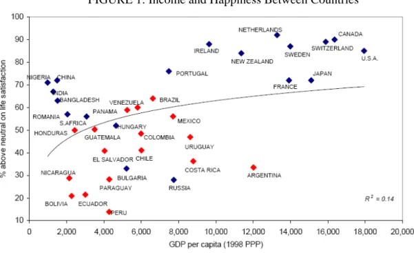
The crux of what is by now a fairly well-known problem is illustrated in Figures 1 to 3. The first figure shows one of a number of different possible plots of average happiness scores by country against GNP per head, as well as a quadratic relationship that represents the best fit between the two variables. The central message of this figure would seem to be that money does buy happiness, at the country level, but only up to a certain point. In particular, richer countries look like they are on a flatter portion of this curve. The cross-section macro evidence thus suggests that increasing GNP per head will be less and less effective in rendering individuals within a country happier on average.

This message is repeated in Figures 2 and 3, which show time-series relationships between income and happiness within countries, as in the original paper by Easterlin (1974). The first shows the data for the US between 1973 and 2004. The sharp growth in real income per capita is not mirrored in happiness. This non-relationship seems to be typical of (rich) OECD countries (although the debate is not entirely settled yet: see Stevenson and Wolfers, 2008), and Figure 3 shows time-series trends in life satisfaction and income for five European countries from 1973 onwards. Again, there is no obvious relationship between the two variables.2

Figures 1 through 3 suggest that greater income over time does not bring about greater happiness, at least in rich countries. One implication would then be that we should stop putting resources into increasing GNP, and divert our attention to something more worthwhile (in happiness terms) instead.

2

All of the analysis discussed in this paper concerns relatively rich countries. There is no doubt that increasing income leads to better outcomes in many countries. Clark et al. (2008a) draw a similar picture to Figures 2 and 3 for East Germany between 1991 and 2002, and find that both income and life satisfaction increased considerably over this period.

One common criticism of the above Figures is that subjective measures of well-being such as life satisfaction or happiness are mostly noise, and can not therefore be used to draw inferences about utility levels neither between individuals nor over time. An arguably powerful reply to this criticism comes from showing that individuals’ current reported well-being is correlated with their future behaviour: satisfaction is a powerful predictor variable, even when a wide variety of other controls are introduced. An early example is Freeman (1978), which showed that current job satisfaction is a better predictor of future quits than are current wages. More generally, satisfaction scores have been shown to predict: life expectancy, morbidity, productivity, quits, absenteeism, unemployment duration, and marriage duration. In this case, subjective well-being must be to some extent comparable between individuals. Were each individual to answer idiosyncratically, it would not be possible to predict the distribution of future observable behaviours across individuals. This literature, together with other work on the validity of subjective measures (cross-rater validity, and physiological and neurological evidence) is surveyed in Clark et al. (2008a).

In this section I consider the evidence that income, Y, is really only weakly correlated with subjective well-being. A number of different authors have carried out work in this area, producing a broadly consistent set of results. The following section will be devoted to identifying variables that really do seem to bring about higher well-being. Here the work is much thinner on the ground, and far more research needs to be carried out before any consensus can be reached.

Both sections will appeal to “micro-data” - data on individuals – whereas Figures 1 through 3 were based on country “macro” averages. The former is likely preferable for a number of different reasons:

1) Well-being scores are ordinal, and so can’t really be averaged. 2) Language/cultural differences (what’s “happy” in French?).

3) There may well be other differences between countries that are correlated with satisfaction. This is a standard omitted variable argument: if something is positively correlated with income but negatively correlated with subjective well-being, then the bivariate correlation between income and well-being will be biased towards zero. This is the case for hours of work or pollution, to give two examples.

4) There are only so many countries, so macro analysis will necessarily always rely on relatively small datasets.

Income Comparisons

The key idea that will be developed in this paper is that individual well-being may very well depend on the “relative” level of many important variables, as well as their absolute level. These relative levels might either be defined with respect to other people, or with respect to oneself in the past.

It is easy to think of examples of comparisons between people over certain consumption goods. Indeed, it often seems as if advertising is explicitly inviting us to get one over others by purchasing the latest model of car, jeans or razors.3 _{Consider the case of two neighbours, A and}

B, who both like cars. We can write their well-being functions in a standard way as then depending on the car that they themselves drive.

WA = W(CarA,...) WB = W(CarB,...)

One of the key questions in the context of social comparisons between the two is whether B’s purchase of a new car will affect A’s well-being and A’s likelihood of buying a new car. The answer is “No” to both questions in standard economic theory.4 _{But if we believe that}

relative standing matters, it is easy to see that B’s new car may well leave A feeling relatively deprived, to which her response will be to invest in some shiny new machinery herself.5 _{If A}

does indeed compare to B, then we can write her welfare function (with respect to cars) as WA = W(CarA/CarB,....). The first element in WA shows how good A’s car is relative to her neighbour’s.

There are now a fair number of papers which have addressed the relationship between Income and Subjective Well-Being (SWB) in exactly the same context as that of the car example above. Broadly, the choice is between two well-being or utility functions:

3

Television advertising during football matches seems to be particularly prone to these kinds of appeals.

4

Leaving to one side any information about the new car that A may learn from repeatedly observing B’s new purchase.

5

A will follow B’s behaviour as long as the comparison part of her utility function is concave. If it is linear, then she will not change her behaviour, and if it is convex, she will do the opposite to B. In all three cases, however, her utility is negatively affected by B’s new car. See Clark and Oswald (1998).

The Standard model: W = W(Y, ....) Comparisons or Relative Utility: W = W(Y/Y*, ....)

The variable Y* here is often called “comparison income”: it is the income to which the individual compares her own, and is often otherwise called reference group income. In the second of the equations above, Y and Y* have been entered in ratio form. In much of the empirical research, Y and Y* are entered separately as right-hand side variables, either in levels or in logs. The general idea is similar across all of the empirical work: if relative income is important, then we expect dW/dY * to be negative – my utility falls as those in my reference group earn more.

The research in this field has used econometric techniques applied to large-scale micro data to model the relationship between some measure of individual well-being and income, both own and that of the reference group. Data are most often from one country only, but sometimes from many different countries. The adjective “large-scale” here means anything between a few thousand to half a million or more. The regression analysis typically includes many other control variables (such as labour force status, marital status, education and health). The aim is to look at the ceteris paribus (all else held constant) relationship between W, Y and Y*.6

To carry out this analysis, we need information on two variables that are arguably only imperfectly measured. The first is the dependent variable, subjective well-being. As argued above, there is now a fairly substantial published literature based on the assumption that respondents’ answers to questions on job or life satisfaction, happiness or general psychological functioning contain useful information that may help us to understand the structure of the individual utility function.

Second, we need a measure of Y*. We thus come back to an old question: Who’s in the reference group? Some likely candidates are:

* The peer group (people who are like me) * Others in the same household

* My spouse or partner * Myself in the past * Friends

6

This is actually less simple than it sounds, as some of the other control variables might depend on income. If higher income buys better health, or even a better chance of getting or staying married, then should we really condition on health or marriage when estimating the relationship between income and well-being?

* Neighbours * Work colleagues

* “Expectations”/”Aspirations”

Almost all of these are horizontal comparisons (i.e. individuals compare to some reference group at a point in time); the comparison to myself in the past is intertemporal or vertical, and raises the possibility of addiction to income.

We almost never have information on which reference group is the most relevant. One of the very few exceptions is Melenberg (1992), who asked respondents directly about the income of the people with whom they often interacted; another is Knight and Song (2006), in which Chinese survey respondents were given a list of options and asked to explicitly state to whom they compared: 68% replied that their main comparison group consisted of individuals in their own village, whereas only 11% stated that their main comparison group consisted of individuals from outside of the village. Wave 3 of the European Social Survey (with data mostly collected in 2006) goes some way toward filling this lacuna. Individuals are first asked “How important is it to you to compare your income with other people’s incomes?” They are then asked “Whose income would you be most likely to compare your own with?”, with responses on a showcard of Work colleagues, Family members, Friends, and Others.7

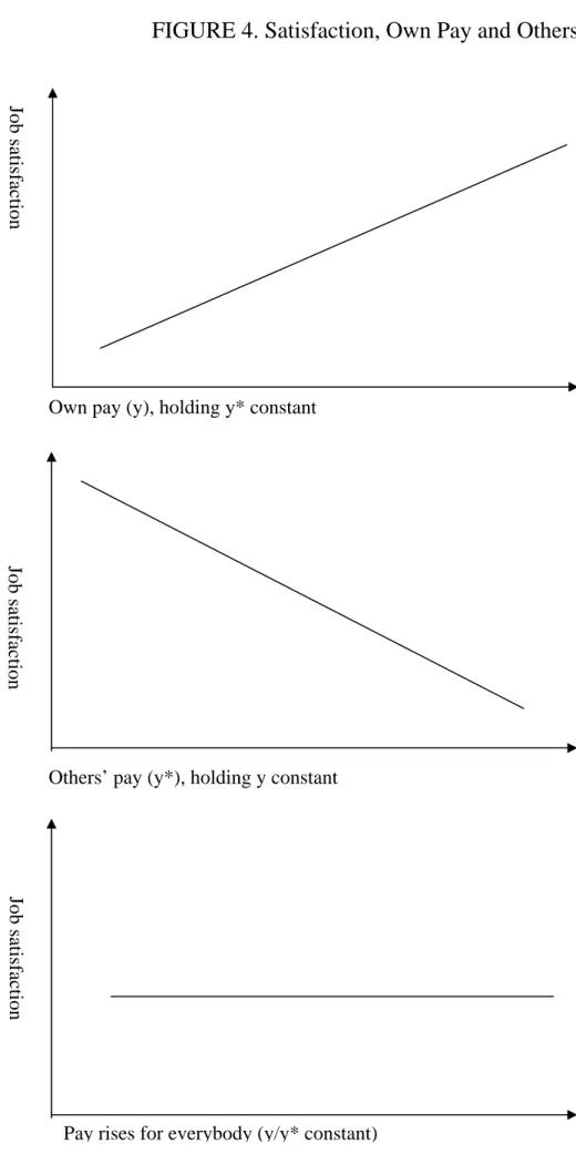
Empirical research has appealed to more or less all of the different definitions of the reference group evoked above. This growing literature is surveyed in Clark et al. (2008a). For example, Clark and Oswald (1996) use the first wave of the British Household Panel Study (BHPS) to look at the relationship between job satisfaction and labour income amongst British employees. The main findings here are that there is evidence that job satisfaction rises with your own income, but falls as the income of the peer group (other people with the same job and demographic characteristics) rises. So we do seem to be in the same situation as in the car example above. Clark (1996) extends this result to partner’s income and the income of other adults in the same household. Luttmer (2005) is a careful attempt to measure comparisons to those with whom individuals are in close geographical proximity; see also Ferrer-i-Carbonell (2005). The broad conclusions from the empirical work modelling subjective well-being as a function of both own income and others’ income are illustrated in Figure 4. The multivariate results suggest that:

7

The relationship between these responses and both life satisfaction and political preferences is explored in Clark and Senik (2008).

* Satisfaction rises with own income, holding others’ income constant. * Job satisfaction falls with others’ income, holding own income constant. * Income rises for everyone may not much affect satisfaction.

This last point is of particular interest, as it recalls the flat part of the cross-country regression line in Figure 1. Note that, from a political economy point of view, we can read the last graph in Figure 4 backwards: reducing everyone’s income leaves no-one worse off. From the first graph, no one person will have an incentive to reduce their own income (Y) if Y* remains unchanged. However, if all incomes fall at the same time then Y/Y* will remain unaffected.8 _{There may then seem to be a role for government coordination, via legislation}9 _or

the tax system, to free up resources for public-good production without making any individual worse off with respect to the utility from their own private consumption. One problematic issue is that any individual who thinks in partial equilibrium (i.e. who sees the effect on their own income, but not that Y* will change as well) will not be in favour of any such intervention.

Wages are habit-forming

Figure 4 was couched in terms of comparisons to others. Comparisons may also take place over time, to the extent that I evaluate my income today in terms of how much I used to earn in the past. The externality here is intertemporal and within-individuals: it is my own past good fortune that reduces my current well-being. As such, individuals adapt to higher incomes. Clark (1999) used BHPS panel data to define Y* as the income of the same individual in the same job one year earlier, and found exactly this type of correlation.

Adaptation to income is of interest for labour economists, as it provides an alternative reading of observed steep wage profiles. Two existing explanations are that productivity profiles are themselves quite steep, or that fast-growing wages reflect an incentive mechanism to avoid shirking (workers effectively post a bond by being underpaid at the beginning of their career, in return for being overpaid at the end of their career – see Akerlof and Katz, 1989). The presence of comparisons to the past implies that, independent of these two concepts, individuals might just simply have a taste for income growth.

8

This does assume that everyone is equally status-conscious with respect to money. If there is heterogeneity in income comparisons, then reducing everyone’s income will hurt those who compare their incomes less.

9

Other Evidence

The statistical analysis of subjective well-being measures in survey data is by no means the only way to show that comparisons take place, although it is the approach that is emphasised here. In terms of income comparisons, there is an enormous amount of work on fairness in experimental economics. Although the fit is not exact,10 _{it is tempting to interpret this research in}

the light of some comparison process. Two examples are Fehr and Schmidt (1999) and Rabin and Charness (2002). In one experiment (Zizzo and Oswald, 2001), individuals are ready to pay to have higher rank. Specifically, they sacrifice part of their own (real) earnings in order to destroy other participants’ earnings.

Another alternative is to ask individuals directly about their preferences between hypothetical outcomes. One strand of this work (Alpizar et al., 2005, Johannsson-Stenman et al., 2002, and Solnick and Hemenway, 1998) has tried to identify social comparisons by asking individuals to choose between states of the world which differ in both the absolute and relative domains. For example, in Solnick and Hemenway, individuals are asked to choose between states A and B, as follows:

A: Your current yearly income is $50,000; others earn $25,000. B: Your current yearly income is $100,000; others earn $200,000.

Here, “others” refers to average wages of other people in the society, and it is emphasised that “prices are what they are currently and prices (the purchasing power of money) are the same in States A and B”. All three papers find that individuals say they are willing to give up absolute income in order to gain status (choosing A over B above). Along the same lines, Frank and Hutchens (1993) and Loewenstein and Sicherman (1991) have shown that individuals express a preference for wage profiles which rise over time, even though these have lower present discounted values than alternative profiles with constant or decreasing wages. People are again essentially prepared to pay to receive upward-sloping profiles.

Finally, a recent literature has looked at neurological evidence for comparisons. Animal studies have shown that neuronal activity is evaluated to relative, rather than absolute, rewards, here represented by different flavours of fruit juice (Cromwell et al., 2005). A novel recent paper (Fließbach et al., 2007) uses MRI techniques to measure the brain activity of pairs of

10

Fairness implies that individuals do not want to be either “underpaid” or “overpaid” relative to others, whereas the well-being literature has typically insisted that individuals like doing better than others, so that the effect of Y* is always negative.

individuals engaged in identical tasks in separate scanners (estimating the number of dots on a computer screen). Success (correctly estimating the number of dots to be greater or lesser than a certain number) entailed a monetary reward, which varied experimentally in size, both in absolute size and relative to the other individual. The condition that interests us here is when both individuals succeed (and therefore both are rewarded). The results show that relative income is significantly correlated with blood oxygenation in the ventral striatum. Brain activity is actually completely relative in this respect (both participants winning 60 produces the same brain activity as both participants winning 30).

The conclusion from this ongoing research programme is then that that there do indeed seem to be significant income comparison effects, both spatially (between groups) and over time with respect to what the individual received in the past. Together, these two might arguably be behind the small effect of aggregate income on aggregate well-being in developed countries.

3. Economic Policy: What Should We Do Now?

A common economic policy conclusion appeals to the research outlined in Section 2 to conclude that “Income and Consumption aren’t making us any happier, so we should spend our time concentrating on X instead”. Some of the candidates for X include:11

* Social activities (marriage, the family, and social capital in general) * Spiritual activities (religion and meaning in life)

* The quality of working life

* Social and Political values (freedom and democracy) * Health

While all of these seem eminently sensible, there would seem to be an element missing from the argument. The work reviewed in Section 2 above did indeed suggest that “There are comparison/habituation effects between income and well-being”. However, the policy prescription “Hence we should be doing something else instead” rests on the untested hypothesis that there are no (or fewer) comparison or habituation effects between the “something else” in question and individual well-being. The remainder of this paper is devoted to evaluating this hypothesis. The potentially depressing conclusion is that, if not pervasive, comparisons to others and habituation seem to form a regular part of economic and social life.

11

Work

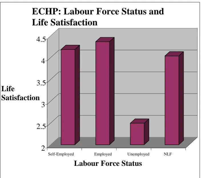
Surely one of the most important elements in individual well-being is the fact of having a job or not, when one wants one. In the Economics literature, along with the relationship between income and happiness, the role of unemployment in individual well-being has been something of a mainstay. Unemployment is strongly negatively correlated with various measures of well-being. Figure 5 illustrates with data from the EHP, where average life satisfaction (on a 1-6 scale, with 6 being the most satisfied) is plotted against labour force status. The unemployed report satisfaction scores that are, on average, two points lower than those given by the employed or the self-employed, which is a very large difference on a six-point scale. This negative relationship persists in regression analysis which controls for the level of income (for example, Clark and Oswald, 1994, and Winkelmann and Winkelmann, 1998): as such, the main effect of unemployment would seem to be non-pecuniary.

In terms of this paper’s subject matter, we are interested in whether there is any evidence of comparisons to unemployment. This question is investigated using multivariate regression analysis, as above, to model the relationship between well-being and unemployment for all individuals of working age. This work has been carried out on British, German, and European (cross-country) panel data.

The main result is that there is indeed some evidence of comparison effects with respect to others’ unemployment. Clark (2003) uses the first seven waves of the British Household Panel Survey to consider the relationship between individual well-being, on the one hand, and regional and household unemployment on the other. While individual unemployment is associated with lower well-being, the size of this negative effect is context-dependent on the local context. Broadly speaking, unemployment hurts less the more there is of it around.12

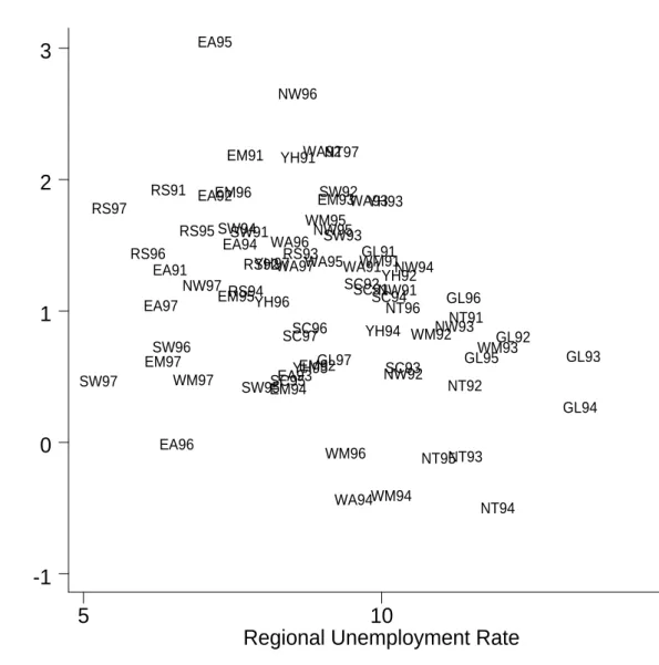
The graphs in Figures 6 and 7 illustrate the main results. Figure 6 shows the bivariate relationship between psychological well-being (as measured by the GHQ-12 score) and regional unemployment. The “Caseness” measure of GHQ runs on a scale of 0 to 12, coded here so that 12 means better psychological functioning. The vertical axis measures the difference in the average GHQ score between the employed and the unemployed: it is therefore a measure of how much worse off the average unemployed person is than the average employed person, or of the

12

Which brings in the possibility of unemployment cultures. George Michael, ex-of Wham!, summed this up perfectly in the lyrics to Wham Rap, which was a hit in the UK in (high unemployment) 1983: “Hey everybody take a look at me, I've got street credibility. I may not have a job, but I have a good time with the boys that I meet down on the line”.

average psychological cost of unemployment. This difference is calculated separately for each of the seven data waves, and for each of the 11 different standard regions in Great Britain (as listed in the note underneath the graph), producing 77 data points in all. The figure on the horizontal axis shows the unemployment rate, by region and by year, matched in from the UK Labour Force Survey. Figure 6 suggests that the psychological cost of unemployment is smaller in regions where the regional unemployment rate is higher.

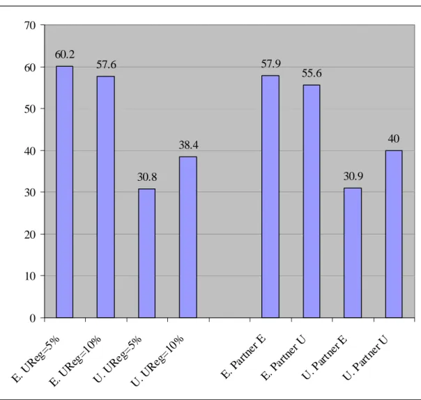
This analysis can be formalised by running multivariate regressions of well-being on own unemployment, regional unemployment, and the interaction between the two, as well as a host of other standard socio-demographic control variables. The results of such regressions are summarised in Figure 7, which presents the predicted well-being levels of individuals in different kinds of labour market situations.13

The left-hand side panel of Figure 7 refers to the relationship between well-being and regional unemployment. The first bar refers to an individual in work (E) in a region with a five per cent unemployment rate. This individual is predicted to have a 60 per cent probability of having high well-being. Moving this employed individual to a region with a higher (10%) unemployment rate slightly reduces their well-being. This relationship is inverted for the unemployed. An unemployed individual in a region with a 5% unemployment rate is predicted to have a 31% chance of having high well-being; moving this unemployed individual to a region with higher unemployment actually increases their well-being (to a figure of 38%).14 _{This result}

concords with findings on suicide and para-suicide rates by the unemployed, which are highest in low-unemployment regions (see Platt and Tansella, 1992).

The right-hand panel repeats this analysis, but for a much tighter reference group: the individual’s spouse. The analysis refers to couples who are both active in the labour market. There are four possible outcomes, given by the combinations of employment and unemployment between the individual and her spouse. The first column shows the probability of high well-being for a worker with an employed spouse (58%); this probability falls to 56% for the employed whose spouse is unemployed. The worst situation is not when both individual and her partner are unemployed, as perhaps might have been imagined, but rather when the individual is unemployed and her partner works.

13

The figures on the vertical axis actually refer to the predicted probability, from an ordered probit equation, that an individual has a “high” level of well-being (a score of 10 to 12 on the 0-12 scale).

14

The regression results actually predict that being employed and being unemployed are associated with the same level of well-being when the regional unemployment rate is somewhere between 20% and 25%, which is however out of sample.

This discussion of social comparisons in the world of work has been confined to the fact of having a job or not. Along the same lines, it would be extremely useful to consider comparisons to others with respect to job characteristics other than income, such as hours of work, size of the office, job disamenities, and so on. Such micro data is often lacking however.

Adaptation to work and life events

A joint project between Economists and Psychologists (Clark et al., 2008b) has considered adaptation to marriage, children, and labour force status using long-run German panel data (the GSOEP). The results are probably best illustrated by a series of graphs. Figures 8 through 13 show how wellbeing evolves around the time of unemployment, marriage, divorce, widowhood, birth of first child, and layoff respectively. The time of the event is shown on the horizontal axis in these graphs as time zero. We illustrate these life satisfaction movements relative to a “baseline” level, which is given by the level of life satisfaction predicted from a fixed effects regression. This predicted value uses information from both observables and unobservables, via the fixed effect. The analysis of life satisfaction relative to baseline of those who at some stage become unemployed (for example) thus controls for any selection effect (unemployment tends to happen to the relatively unhappy). In words, these graphs map out the profile of life satisfaction of someone who becomes unemployed (for example) relative to the “baseline” profile that we would have calculated for them had that unemployment not occurred.

A last point is that the estimated coefficients depicted in the figures show adaptation to marriage, for example, for those who stayed married up to the time in question (the effect of married at t+4 is the life satisfaction of those who married at t, and are still married at t+4). We could also have evaluated the life satisfaction at t+4 of all of those who married at t, regardless of whether they were now married, divorced etc four years later. This latter approach picks up both adaptation to marriage and the normal drop in life satisfaction upon marriage termination, and therefore would in general, yield greater “bouncing back” than the graphs we show here (simply because some marriages fail, and the unemployed find new jobs).

The graphs show that complete adaptation for the majority of the six events (marriage, divorce, widowhood, birth of first child, and layoff). However, there is little evidence of adaptation to unemployment for men (see also Clark, 2006, for corroborative unemployment results from different datasets). In general, men are more affected by labour market events (unemployment and layoffs) than are women. Apart from unemployment, the phenomenon of adaptation appears to be widespread for the events analysed.

Health

We next turn to comparisons with respect to individual health status, both with respect to others and with respect to the past. Regarding the former, we would want to show that the well-being impact of poor health is reduced if the reference group experiences poorer health as well. Research in this area is still very recent, and the three papers mentioned below all date from the year of writing. Powdthavee (2008) considers the relationship between physical health problems and (subjective) self-assessed health. Using BHPS data, he is able to show that the strength of the relationship between own health problems and own subjective health is reduced for those who live with other people who also have health problems. This is consistent with comparison effects in subjective health. The size of this comparison effect is however only relatively small.

Comparison effects are also investigated in two recent papers which look at individual body shape. Blanchflower, Oswald and van Landeghem (2008) show that feelings of being overweight fall with the average weight of the peer group (measured at the country*age group*sex level) in Eurobarometer data; they also have some speculative results using GSOEP data that the effect of own BMI on life satisfaction is smaller in region*year cells with higher levels of BMI.

Clark and Etilé (2008) is along somewhat the same lines, and uses both GSOEP and BHPS data to analyse the relationship between individual well-being on the one hand, and both own and partner’s BMI on the other hand. It is shown that, at least after a certain point, own BMI and well-being are negatively related. However, the strength of this relationship is mitigated by partner’s BMI. In the BHPS data, an individual in a couple where both are obese reports a similar mental stress level to an individual in a couple where neither is obese.

A number of recent papers have considered adaptation to health problems or to disability. This is likely to be a growing research field. Oswald and Powdthavee (2008) use BHPS and GSOEP data and find partial adaptation to disability using a fixed-effect (within-subject) approach similar to that of Clark et al. (2008b) in the previous sub-section. As Oswald and Powdthavee note, their results are not the same as those in Lucas (2007), who uses the same datasets but a different analytic approach, and finds little or no adaptation to disability.15 _With

respect to specific health problems, Wu (2001) uses two waves of US Health and Retirement Study data and estimates what are essentially first-difference health equations. He has

15

This disagreement is also found in the adaptation to marriage literature. Analysis of the same GSOEP data produces full adaptation in a fixed-effect model (Clark et al., 2008b) but only partial adaptation in a Multi-Level Model (Lucas et al., 2003).

information on whether the individual experienced a new heart condition between the two waves, but also on whether they had had a heart condition prior to the first wave. His test of adaptation consists in seeing whether a new heart condition has a smaller effect on health for those who had already experienced heart problems. He finds significant evidence of this effect for both self-reported health and a measure of emotional health (“What about your emotional health — how good you feel or how stressed, anxious, or depressed you feel?” answered on a one-to-five scale), and argues that individuals do adapt to heart conditions. Last, Riis et al. (2005) use an experienced sample measure, and find that the well-being reported by hemodialysis patients is similar to that of the healthy.

Social Capital

The last two substantive parts of this section consider comparisons with perhaps more nebulous aspects of the “good life”. The first is social capital, as emphasised by Putnam (2000). While a growing number of economists seem to consider that social capital is an important variable in explaining economic outcomes, there is as yet no unambiguous way of measuring it. As is often the case, the definition used in my own research has been dictated by data availability. I consider social capital as activity in organisations (social engagement), rather than some measure of trust. In this respect I follow Glaeser et al. (2002).

In Waves Seven and Nine of the BHPS, individuals are asked whether they are active in the following organisations: ¾ Political party ¾ Trade union ¾ Environmental group ¾ Parents association ¾ Tenants group ¾ Religious group ¾ Voluntary group

¾ Other community group ¾ Social group

¾ Sports club ¾ Women’s institute ¾ Women’s group ¾ Other organisation

The Yes/No answers to these questions can be summed to produce a social capital activity score which runs from 0 to 13. Equally, in Waves 8 and 10 individuals are asked about the intensity with which they carry out the following activities:

¾ Walk/swim/play sport ¾ Watch live sport ¾ Go to the cinema ¾ Go to theatre/concert ¾ Eat out

¾ Go out for a drink ¾ Work in garden

¾ Do DIY, car maintenance ¾ Attend evening classes ¾ Attend local groups ¾ Do voluntary work

The replies are recoded so that a value of one refers to “At least once a month” or more often, and zero to less often than once a month. The sum of these recoded answers provides a social capital intensity score which runs from 0 to 11. We therefore have two social capital measures, referring to activity (what you do), and intensity (how often you do it).

Regression analysis of life satisfaction shows that, as expected, those with more social capital are more satisfied with their lives. This holds for both activity and intensity. We should however be aware of the difficulty of establishing causality in this relationship. Using the household aspect of the BHPS, we can then match in the social capital activity of all of the other adults who live in the same household as the respondent.

The regression results in Table 1 below are consistent with BHPS respondents evaluating their social capital activity relatively to those with whom they are in close contact (other household members). In particular, Individuals like to live in households with active members but they also want to be more active than anyone else: there is a life-satisfaction boost from being the most socially-active person in the household.

It is also possible to use information from the two separate waves to consider adaptation to social capital. Is the effect of a given amount of social activity at Wave Nine smaller for those who were more active at Wave Seven? Regression analysis provided no evidence of such an adaptation effect, although social capital is arguably only inaccurately measured here, and only two data points over time may be insufficient for a serious analysis of adaptation.

Religion

The last type of social comparison considered in detail here is religious. It is by now well-established that the religious report higher subjective well-being scores than do the non-religious. In Clark and Lelkes (2008), we appeal to data from the first three waves of the

European Social Survey to consider whether the life satisfaction boost from my own religiosity depends on how religious my neighbours are.

We find that own religious behaviour is positively correlated with individual life satisfaction, controlling for demographic characteristics and country fixed effects. Average religious behaviour in the region (defined at the NUTS2 level) also has a positive impact: people are happier in more religious regions. The other side of the coin is that respondents report lower satisfaction scores in regions where there is a higher percentage of “atheists” (those who say they do not belong to any religious denomination). However, contrary to some of the previous results, this positive spillover from others’ religious behaviour did not depend on the individual’s own religiosity. Those who reported belonging to a particular religious denomination were less satisfied as the percentage of atheists in the region increased. However, atheists were less satisfied living in less religious regions as well. This type of generalised spillover from religion is different in nature to that of unemployment discussed above, where higher regional unemployment reduced the being of the employed but increased the well-being of the unemployed.

We further investigated religious spillovers by asking whether there were ever any circumstances in which one individual’s religiosity might reduce the well-being of another individual in the same region. We did so by considering the role of the dominant religion: even though everyone likes living in religious regions, do the religious receive a larger satisfaction return when they belong to the dominant religion in the region? The results are shown in Table 2. Catholics are indeed significantly more satisfied (at the 1% level) when Catholicism is dominant, with respect to both measures of dominance: being the majority religion in the region, including atheists, and being in the absolute majority (i.e. over 50% of the population). The results for Protestants are similar, although only significant for the first measure.

The results in Table 2 do suggest one avenue in which others’ religion can have a negative spillover effect. Any expansion of one religious denomination will reduce the life satisfaction of those belonging to another religion if it causes the latter to lose their dominant position.

4. Conclusion

There is now a considerable amount of work which has tested whether individual well-being exhibits relative or comparison effects with respect to income. This chapter has argued that, in the interests of both science and public policy, the same energy should be devoted to looking for analogous comparison effects in other areas of economic and social life. Table 3 is a

rough and ready attempt to summarise the position of our current knowledge regarding such comparisons, both with respect to others and to the past. Two key points should be underlined in this table.

The first is that many of the policy statements that have issued from research on subjective well-being have considered only the first line of this table: social comparisons and adaptation seem rife with respect to income, so we should change our priorities from income to something else. To be sure that this policy prescription is germane, we need to establish that comparisons and adaptations are not present (or are at least less strong) in the alternative priority areas that are put forward. The general message from the empirical work that has been briefly surveyed in this paper is that we really should not take this for granted. We have not found evidence of comparisons and adaptation in all areas of life, but there is certainly evidence consistent with such phenomena in a number of different non-income fields.

The second point is that our knowledge is still incomplete. Even in terms of the domains that appear in Table 2, there are an impressive number of question marks. And we can always imagine adding new elements to the table.

Related to the above, it is perhaps naïve to imagine that there is only one relationship between my own well-being and others’ outcomes, in all contexts and for all individuals. For example, a recent small literature has underlined that others’ income may well be positively related to my own well-being under certain conditions. This could be because it provides information about my own potential future earnings (in an application of Hirschman’s tunnel effect: see Senik, 2004, and Clark et al., 2008c, for example), or because richer very close neighbours help in the provision of local public goods (as suggested in Clark et al., 2008d). With respect to individual heterogeneity, recent work has suggested substantial differences in individual adjustment profiles following shocks (Bonanno et al., 2002, Mancini et al., 2008), and it is likely that the same heterogeneity applies with respect to the strength of comparison to others. Research in these areas is still in its infancy.

One of the interesting uses of subjective well-being data has arguably been to reveal information about the structure of the utility function. An important application of this research will be to determine which policy variables have significant and long-lasting effects on subjective well-being, without suffering from status effects or adaptation. This will likely be one of the greatest contributions of well-being research to the economic policy debate.

FIGURE 1: Income and Happiness Between Countries

FIGURE 2: Happiness and Real Income Per Capita in the US, 1973-200416 0 0.5 1 1.5 2 2.5 3 1973 1977 1981 1985 1989 1993 1998 2003 Year Aver age Hap p in ess 0 10000 20000 30000 40000 R eal Income P er C api ta (Cons ta nt 2 000 U S $ )

Happiness Real Income Per Capita

FIGURE 3: Life Satisfaction in Five European Countries, 1973-200417

0 0.5 1 1.5 2 2.5 3 3.5 4 1973 1977 1980 1983 1986 1988 1990 1993 1996 2000 2004 Year Aver age L if e S atisf action

UK France Germany Italy Netherlands

16

Published in Clark et al. (2008a). Source: World Database of Happiness and Penn World Tables. Average reply to the following question: ‘Taken all together, how would you say things are these days? Would you say that you are…?’ Responses are coded as (3) Very Happy, (2) Pretty Happy, and (1) Not too Happy. Happiness data are drawn from the General Social Survey.

17

Published in Clark et al. (2008a). Source: World Database of Happiness. Average responses to the following question: ‘On the whole how satisfied are you with the life you lead’. Responses are coded as (4) Very Satisfied, (3) Fairly Satisfied, (2) Not Very Satisfied, and (1) Not at all Satisfied. Life satisfaction data are drawn from the

FIGURE 4. Satisfaction, Own Pay and Others’ Pay

Own pay (y), holding y* constant

Jo b s at is fa ct io n

Others’ pay (y*), holding y constant

Jo b s at is fa ct io n

Pay rises for everybody (y/y* constant) Eurobarometer Survey.

Figure 5. Life Satisfaction and Labour Force Status.

2

2.5

3

3.5

4

4.5

Life

Satisfaction

Self-Employed Employed Unemployed NLF

Labour Force Status

ECHP: Labour Force Status and

Life Satisfaction

Figure 6. The Well-Being Gap between those in Work and the Unemployed

(GHQ

-GHQ

) and Regional Unemployment Rates.

BHPS Waves One to Seven. (Eleven Regions)

GHQ

Diff

erence

Regional Unemployment Rate

5 10 15 -1 0 1 2 3 GL91 GL92 GL93 GL94 GL95 GL96 GL97 RS91 RS92RS93 RS94 RS95 RS96 RS97 SW91 SW92 SW93 SW94 SW95 SW96 SW97 EA91 EA92 EA93 EA94 EA95 EA96 EA97 EM91 EM92 EM93 EM94 EM95 EM96 EM97 WM91 WM92 WM93 WM94 WM95 WM96 WM97 NW91 NW92 NW93 NW94 NW95 NW96 NW97 YH91 YH92 YH93 YH94 YH95 YH96 YH97 NT91 NT92 NT93 NT94 NT95 NT96 NT97 WA91 WA92 WA93 WA94 WA95 WA96 WA97 SC91 SC92 SC93 SC94 SC95 SC96 SC97

Key: GL = Greater London, RS = Rest of the South East, SW = South West, EA = East Anglia, EM = East Midlands, WM = West Midlands, NW = North West, YH = Yorkshire and Humberside, NT = North, WA = Wales, SC = Scotland.

Figure 7. Well-Being and a) Regional Unemployment, and b) Partner’s

Unemployment.

Notes to Figures 8-13: Published in Clark et al. (2008b).

*

Table 1. Life Satisfaction and Social Capital Regressions

Own Social Capital Activity

-0.001

(.021)

Other Household Members’

0.062 *

Social Capital Activity

(.025)

More Active than Other

0.054 *

Household Members

(.026)

Notes: Data from Waves 7 and 9 of the BHPS. Ordered probit estimates. The

models include personal controls and region and wave fixed effects. Standard

errors in parentheses. * significant at the 5% level.

Table 2. Spillover effects of belonging to the dominant denomination

Protestants

Roman

Catholics

Belongs to dominant

denomination

(incl. atheists)

0.186**

(0.046)

0.104*

(0.041)

Belongs to absolute

majority denomination

(incl. atheists)

0.077

(0.047)

0.173**

(0.045)

Observations

14183 14183 26712

26712

Notes: Based on European Social Survey data, Waves 1-3. Dominant

denomination defined at the regional level. Ordered logit estimates. The models

include personal controls and country fixed effects. Standard errors in parentheses.

* significant at the 5% level; ** significant at the 1% level. Source: Clark and

Lelkes (2008).

Table 3. Social Comparisons and Adaptation in Economic and Social Life

Horizontal Intertemporal

Comparisons Comparisons

(Status) (Adaptation)

Income Yes Yes

Unemployment Yes No

Marriage/Divorce ? Yes

Health Perhaps? Partial?

Social Activities Perhaps? No?

Freedom ? ?

REFERENCES

Akerlof, G.A., and Katz, L.F. (1989). “Worker's Trust Funds and the Logic of Wage Profiles”. Quarterly Journal of Economics, 104, 525-536.

Alpizar, F., Carlsson, F. and Johansson-Stenman, O. (2005). “How much do we care about Absolute versus relative income and consumption?”. Journal of Economic Behavior and Organization, 56, 405-421.

Blanchflower, D.G., Oswald, A.J., and Van Landeghem, B. (2008). “Imitative Obesity and Relative Utility”. NBER Working Paper No.14377.

Bonanno, G.A., Wortman, C.B., Lehman, D.R., Tweed, R.G., Haring, M., Sonnega, J., Carr, D., and Nesse, R.M. (2002). “Resilience to loss and chronic grief: A prospective study from preloss to 18-months postloss”. Journal of Personality and Social Psychology, 83, 1150-1164.

Clark, A.E. (1996). “L'utilité est-elle relative? Analyse à l'aide de données sur les ménages”. Economie et Prévision, 121, 151-164.

Clark, A.E. (1999). “Are Wages Habit-Forming? Evidence from Micro Data”. Journal of Economic Behavior and Organization, 39, 179-200.

Clark, A.E. (2003). “Unemployment as a Social Norm: Psychological Evidence from Panel Data”. Journal of Labor Economics, 21, 323-351.

Clark, A.E. (2006). “A Note on Unhappiness and Unemployment Duration”. Applied Economics Quarterly, 52, 291-308.

Clark A., Diener E., Georgellis T. and Lucas R. (2008a). “Lags and Leads in Life Satisfaction: A Test of the Baseline Hypothesis”, Economic Journal, 118, 222-243.

Clark, A.E., and Etilé, F. (2008). “Happy House: Spousal Weight and Individual Well-Being”. PSE, mimeo.

Clark, A.E., Frijters, P., and Shields, M. (2008b). “Relative Income, Happiness and Utility: An Explanation for the Easterlin Paradox and Other Puzzles”. Journal of Economic Literature, 46, 95-144.

Clark, A.E., Kristensen, N., and Westergård-Nielsen, N. (2008c). “Job Satisfaction and Co-worker Wages: Status or Signal?”. Economic Journal, forthcoming.

Clark, A.E., Kristensen, N., and Westergård-Nielsen, N. (2008d). “Economic Satisfaction and Income Rank in Small Neighbourhoods”. Journal of the European Economic Association, forthcoming.

Clark, A.E., and Lelkes, O. (2008). “Let us Pray: Religious Interactions in Life Satisfaction”. PSE, mimeo.

Clark, A.E., and Oswald, A.J. (1994). “Unhappiness and Unemployment”. Economic Journal,

104, 648-659.

Clark, A.E., and Oswald, A.J. (1996). “Satisfaction and Comparison Income”. Journal of Public Economics, 61, 359-81.

Clark, A.E., and Oswald, A.J. (1998). "Comparison-concave Utility and Following Behaviour in Social and Economic Settings". Journal of Public Economics, 70, 133-155.

Clark, A.E., and Senik, C. (2008). “The Anatomy of Envy. The Intensity, Direction and Effects of Income Comparisons”. PSE, mimeo.

Cromwell, H., Hassani, O. and Schultz, W. (2005). Relative reward processing in primate striatum. Experimental Brain Research, vol. 162, pp. 520–525.

Di Tella, R., and MacCulloch, R. (2006). “Some Uses of Happiness Data in Economics”. Journal of Economic Perspectives, 20, 25-46.

Dolan, P. and Metcalfe, R. (2007). “Valuing Non-Market Goods: A Comparison of Preference-Based and Experience-Preference-Based Approaches”. Tanaka Business School, Imperial College London, mimeo.

Easterlin, R. (1974). “Does economic growth improve the human lot? Some empirical evidence”. In David, R. and Reder, R. (Eds.), Nations and Households in Economic Growth: Essays in Honor of Moses Abramovitz. New York: Academic Press.

Fehr, E., and Schmidt, K. (1999). “A Theory of Fairness, Competition and Cooperation”. Quarterly Journal of Economics, 114, 817-868.

Ferrer-i-Carbonell, A. (2005). “Income and well-being: an empirical analysis of the comparison income effect”. Journal of Public Economics, 89, 997-1019.

Fließbach, K., Weber, B., Trautner, P., Dohmen, T., Sunde, U., Elger, C., and Falk, A. (2007). “Social comparison affects reward-related brain activity in the human ventral striatum”. Science, 318, 1305-1308.

Frank, R.H. and Hutchens, R.M. (1993). “Wages, seniority, and the demand for rising consumption profiles”. Journal of Economic Behavior and Organization, 21, 251-276. Frey, B.S., and Stutzer, A. (2000). “Happiness, Economy and Institutions”. Economic Journal,

110, 918-938.

Glaeser, E., Laibson, D., and Sacerdote, B. (2002). “An Economic Approach to Social Capital”. Economic Journal, 112, 437-458.

Graham, C., & Pettinato, S. (2002). Happiness and Hardship. Opportunity and Insecurity in New Market Economies. Washington D.C.: Brookings Institution Press.

Gruber, J., and Mullainathan, S. (2005). “Do Cigarette Taxes Make Smokers Happier?”. Advances in Economic Analysis and Policy, 5, Article 4.

Johannsson-Stenman, O., Carlsson, F., and Daruvala, D. (2002). “Measuring future grandparents' preferences for equality and relative standing”. Economic Journal, 112, 362-383.

Kahneman, D., Krueger, A., Schkade, D., Schwarz, N., and Stone, A. (2004). “Toward National Well-Being Accounts”. American Economic Review, 94, 429-434.

Knight, J., and Song, L. (2006). “Subjective Well-being and its Determinants in Rural China”. University of Nottingham, mimeo.

Layard, R. (2005). Happiness: Lessons from a New Science. London: Penguin.

Loewenstein, G. and Sicherman, N. (1991). “Do workers prefer increasing wage profiles?” Journal of Labor Economics, 9, 67-84.

Lucas, R., Clark, A.E., Georgellis, Y., and Diener, E. (2003). “Re-Examining Adaptation and the Setpoint Model of Happiness: Reaction to Changes in Marital Status”. Journal of Personality and Social Psychology, 84, 527-539.

Lucas, R. (2007). “Long-term disability is associated with lasting changes in subjective well being: Evidence from two nationally representative longitudinal studies”. Journal of Personality and Social Psychology, 92, 717-730.

Luttmer, E. (2005). “Neighbors as Negatives: Relative Earnings and Well-Being”. Quarterly Journal of Economics, 120, 963-1002.

Mancini, A., Bonanno, G., and Clark, A.E. (2008). “Stepping Off the Hedonic Treadmill: Individual Differences in Response to Marriage, Divorce, and Spousal Bereavement”. Columbia University, mimeo.

Melenberg, B. (1992). “Micro-econometric Models of Consumer Behaviour and Welfare”. Tilburg University, mimeo.

Oswald, A.J., and Powdthavee, N. (2008). “Does happiness adapt? A longitudinal study of disability with implications for economists and judges”. Journal of Public Economics,

92, 1061-1077.

Platt, S.M.R. and Tansella, M. (1992). “Suicide and Unemployment in Italy: Description, Analysis and Interpretation of Recent Trends”. Social Science and Medicine, 34, 1191-1201.

Putnam, R.D. (2000). Bowling Alone. New York: Simon and Schuster.

Powdthavee, N. (2008). “Ill-Health as a Social Norm: Longitudinal Evidence on Self-Assessed Health”. Social Science and Medicine, forthcoming.

Rabin, M., and Charness, G. (2002). “Understanding Social Preferences with Simple Tests”. Quarterly Journal of Economics, 117, 817-869.

Riis, J., Loewenstein, G., Baron, J., Jepson, C., Fagerlin, A., and Ubel, P. (2005). “Ignorance of Hedonic Adaptation to Hemodialysis: A Study Using Ecological Momentary Assessment”. Journal of Experimental Psychology: General, 134, 3–9.

Senik, C. (2004). “When Information Dominates Comparison: A Panel Data Analysis Using Russian Subjective Data”. Journal of Public Economics, 88, 2099-2123.

Solnick, S.J. and Hemenway, D. (1998). “Is more always better? A survey on positional concerns”. Journal of Economic Behavior and Organization, 37, 373-383.

Stevenson, B., and Wolfers, J. (2008). “Economic Growth and Subjective Well-Being: Reassessing the Easterlin Paradox”. Brookings Papers on Economic Activity, Spring. Van Praag, B.M.S., and Baarsma, B.E. (2005). “Using Happiness Surveys to Value Intangibles:

the Case of Airport Noise”. Economic Journal, 115, 224-246.

Winkelmann, L., and Winkelmann, R. (1998). “Why Are the Unemployed So Unhappy? Evidence from Panel Data”. Economica, 65, 1-15.

Wu, S. (2001). “Adapting to Heart Conditions: A Test of the Hedonic Treadmill”. Journal of Health Economics, 20, 495-508.

Zizzo, D.J., and Oswald, A.J. (2001). “Are People Willing to Pay to Reduce Others' Incomes?”. Annales d'Economie et de Statistique, 63-64, 39-65.