HAL Id: hal-00328451
https://hal.archives-ouvertes.fr/hal-00328451
Submitted on 17 Jul 2006
HAL is a multi-disciplinary open access
archive for the deposit and dissemination of
sci-entific research documents, whether they are
pub-lished or not. The documents may come from
teaching and research institutions in France or
abroad, or from public or private research centers.
L’archive ouverte pluridisciplinaire HAL, est
destinée au dépôt et à la diffusion de documents
scientifiques de niveau recherche, publiés ou non,
émanant des établissements d’enseignement et de
recherche français ou étrangers, des laboratoires
publics ou privés.
compared with GOME retrievals for the year 2000
T. P. C. van Noije, H. J. Eskes, F. J. Dentener, D. S. Stevenson, K. Ellingsen,
M. G. Schultz, O. Wild, M. Amann, C. S. Atherton, D. J. Bergmann, et al.
To cite this version:
T. P. C. van Noije, H. J. Eskes, F. J. Dentener, D. S. Stevenson, K. Ellingsen, et al.. Multi-model
ensemble simulations of tropospheric NO2 compared with GOME retrievals for the year 2000.
Atmo-spheric Chemistry and Physics, European Geosciences Union, 2006, 6 (10), pp.2979.
�10.5194/ACP-6-2943-2006�. �hal-00328451�
www.atmos-chem-phys.net/6/2943/2006/ © Author(s) 2006. This work is licensed under a Creative Commons License.
Chemistry
and Physics
Multi-model ensemble simulations of tropospheric NO
2
compared
with GOME retrievals for the year 2000
T. P. C. van Noije1, H. J. Eskes1, F. J. Dentener2, D. S. Stevenson3, K. Ellingsen4, M. G. Schultz5, O. Wild6,7, M. Amann8, C. S. Atherton9, D. J. Bergmann9, I. Bey10, K. F. Boersma1, T. Butler11, J. Cofala8, J. Drevet10,
A. M. Fiore12, M. Gauss4, D. A. Hauglustaine13, L. W. Horowitz12, I. S. A. Isaksen4, M. C. Krol2,14, J.-F. Lamarque15, M. G. Lawrence11, R. V. Martin16,17, V. Montanaro18, J.-F. M ¨uller19, G. Pitari18, M. J. Prather20, J. A. Pyle7,
A. Richter21, J. M. Rodriguez22, N. H. Savage7, S. E. Strahan22, K. Sudo6, S. Szopa13, and M. van Roozendael19
1Royal Netherlands Meteorological Institute, De Bilt, The Netherlands
2European Commission, Joint Research Centre, Institute for Environment and Sustainability, Ispra, Italy
3University of Edinburgh, School of Geosciences, Edinburgh, UK
4University of Oslo, Department of Geosciences, Oslo, Norway
5Max Planck Institute for Meteorology, Hamburg, Germany
6Frontier Research Center for Global Change, JAMSTEC, Yokohama, Japan
7University of Cambridge, Centre for Atmospheric Science, UK
8International Institute for Applied Systems Analysis, Laxenburg, Austria
9Lawrence Livermore National Laboratory, Atmospheric Science Division, Livermore, USA
10Ecole Polytechnique F´ed´eral de Lausanne, Switzerland
11Max Planck Institute for Chemistry, Mainz, Germany
12Geophysical Fluid Dynamics Laboratory, NOAA, Princeton, NJ, USA
13Laboratoire des Sciences du Climat et de l’Environnement, Gif-sur-Yvette, France
14Space Research Organisation Netherlands, Utrecht, The Netherlands
15National Center of Atmospheric Research, Atmospheric Chemistry Division, Boulder, CO, USA
16Department of Physics and Atmospheric Science, Dalhousie University, Halifax, Nova Scotia, Canada
17Smithsonian Astrophysical Observatory, Cambridge, MA, USA
18Universit`a L’Aquila, Dipartimento di Fisica, L’Aquila, Italy
19Belgian Institute for Space Aeronomy, Brussels, Belgium
20Department of Earth System Science, University of California, Irvine, USA
21Institute of Environmental Physics, University of Bremen, Bremen, Germany
22Goddard Earth Sciences and Technology Center, Maryland, Washington, D.C., USA
Received: 16 December 2005 – Published in Atmos. Chem. Phys. Discuss.: 12 April 2006 Revised: 27 June 2006 – Accepted: 28 June 2006 – Published: 17 July 2006
Abstract. We present a systematic comparison of
tropo-spheric NO2 from 17 global atmospheric chemistry
mod-els with three state-of-the-art retrievals from the Global Ozone Monitoring Experiment (GOME) for the year 2000. The models used constant anthropogenic emissions from IIASA/EDGAR3.2 and monthly emissions from biomass burning based on the 1997–2002 average carbon emissions from the Global Fire Emissions Database (GFED). Model output is analyzed at 10:30 local time, close to the overpass time of the ERS-2 satellite, and collocated with the measure-ments to account for sampling biases due to incomplete spa-Correspondence to: T. P. C. van Noije
(noije@knmi.nl)
tiotemporal coverage of the instrument. We assessed the im-portance of different contributions to the sampling bias: cor-relations on seasonal time scale give rise to a positive bias of 30–50% in the retrieved annual means over regions dom-inated by emissions from biomass burning. Over the indus-trial regions of the eastern United States, Europe and eastern China the retrieved annual means have a negative bias with significant contributions (between –25% and +10% of the
NO2column) resulting from correlations on time scales from
a day to a month. We present global maps of modeled and
retrieved annual mean NO2column densities, together with
the corresponding ensemble means and standard deviations for models and retrievals. The spatial correlation between
the individual models and retrievals are high, typically in the range 0.81–0.93 after smoothing the data to a common res-olution. On average the models underestimate the retrievals in industrial regions, especially over eastern China and over the Highveld region of South Africa, and overestimate the retrievals in regions dominated by biomass burning during the dry season. The discrepancy over South America south of the Amazon disappears when we use the GFED emissions specific to the year 2000. The seasonal cycle is analyzed in detail for eight different continental regions. Over regions dominated by biomass burning, the timing of the seasonal cycle is generally well reproduced by the models. However, over Central Africa south of the Equator the models peak one to two months earlier than the retrievals. We further evaluate
a recent proposal to reduce the NOxemission factors for
sa-vanna fires by 40% and find that this leads to an improvement of the amplitude of the seasonal cycle over the biomass burn-ing regions of Northern and Central Africa. In these regions the models tend to underestimate the retrievals during the wet season, suggesting that the soil emissions are higher than as-sumed in the models. In general, the discrepancies between models and retrievals cannot be explained by a priori profile assumptions made in the retrievals, neither by diurnal varia-tions in anthropogenic emissions, which lead to a marginal
reduction of the NO2abundance at 10:30 local time (by 2.5–
4.1% over Europe). Overall, there are significant differences among the various models and, in particular, among the three retrievals. The discrepancies among the retrievals (10–50% in the annual mean over polluted regions) indicate that the previously estimated retrieval uncertainties have a large sys-tematic component. Our findings imply that top-down
esti-mations of NOxemissions from satellite retrievals of
tropo-spheric NO2are strongly dependent on the choice of model
and retrieval.
1 Introduction
Nitrogen dioxide (NO2) plays a key role in tropospheric
chemistry with important implications for air quality and
cli-mate change. On the one hand, tropospheric NO2is
essen-tial for maintaining the oxidizing capacity of the atmosphere.
Photolysis of NO2 during daytime is the major source of
ozone (O3)in the troposphere and photolysis of O3 in turn
initializes the production of the hydroxyl radical (OH), the main cleansing agent of the atmosphere. On the other hand,
NO2as well as O3are toxic to the biosphere and may cause
respiratory problems for humans. Moreover, NO2may react
with OH to form nitric acid (HNO3), one of the main
com-ponents of acid rain. As a greenhouse gas, NO2contributes
significantly to radiative forcing over industrial regions, es-pecially in urban areas (Solomon et al., 1999; Velders et al.,
2001). Although the direct contribution of tropospheric NO2
to global warming is relatively small, emissions of nitrogen
oxides (NOx≡NO+NO2)affect the global climate indirectly
by perturbing O3and methane (CH4)concentrations.
Over-all, indirect long-term global radiative cooling due to
de-creases in CH4and O3dominates short-term warming from
regional O3 increases (Wild et al., 2001; Derwent et al.,
2001; Berntsen et al., 2005).
The main sources of tropospheric NOxare emissions from
fossil fuel combustion, mostly from power generation, road transport as well as marine shipping, and industry. Other im-portant surface sources are emissions from biomass burning, mostly from savanna fires and tropical agriculture, and from microbial activity in soils; important sources in the free tro-posphere are emissions from lightning and aircraft. Minor
sources are due to oxidation of ammonia (NH3)by the
bio-sphere and transport from the stratobio-sphere. By far the
ma-jority of the NOxis emitted as NO, but photochemical
equi-libration with NO2takes place within a few minutes. The
principal sink of tropospheric NOxis oxidation to HNO3by
reaction of NO2with OH during daytime and by reaction of
NO2with O3followed by hydrolysis of N2O5on aerosols at
night (Dentener and Crutzen, 1993; Evans and Jacob, 2005).
The resulting NOxlifetime in the planetary boundary layer
varies from several hours in the tropics to 1–2 days in the ex-tratropics during winter (Martin et al., 2003b) and increases to a few days in the upper troposphere. Long-range
trans-port of NOxmay take place in the form of
peroxyacetylni-trate (PAN), which is formed by photochemical oxidation of
hydrocarbons in the presence of NOx. As PAN is stable at
low temperatures, it may be transported over large distances
through the middle and upper troposphere and release NOx
far from its source by thermal decomposition during subsi-dence.
Because of the relatively heterogeneous distribution of its sources and sinks in combination with its short lifetime, the
concentration of tropospheric NOxis highly variable in space
and time. Monitoring of NO2therefore requires covering a
broad spectrum of spatial and temporal scales, using a com-bination of ground-based and air-borne measurements, as well as those derived from satellites. During the last decade, observations from space have provided a wealth of
informa-tion on the global and regional distribuinforma-tion of NO2on daily
to multi-annual time scales. We now have nearly 10 years of
tropospheric NO2 data from the Global Ozone Monitoring
Experiment (GOME) instrument on board the second Euro-pean Remote Sensing (ERS-2) satellite, which was launched by the European Space Agency (ESA) in April 1995. ERS-2 flies in a sun-synchronous polar orbit, crossing the equator at 10:30 local time. GOME is a nadir-viewing spectrometer operating in the ultraviolet and visible part of the spectrum, and has a forward-scan ground pixel size of 320 km across track by 40 km along track. Global coverage of the obser-vations is reached within three days. Global tropospheric
NO2 columns have been retrieved from GOME for the
pe-riod January 1996–June 2003; since 22 June 2003 data cov-erage is limited to Europe, the North Atlantic, western North
America, and the Arctic (due to failure of the ERS-2 tape
recorder). Higher resolution tropospheric NO2retrieval data
have recently become available from the Scanning Imag-ing Absorption Spectrometer for Atmospheric Chartography (SCIAMACHY) instrument on board the ESA Envisat satel-lite (launched in March 2002) and from the Ozone Monitor-ing Instrument (OMI) on board the NASA Earth ObservMonitor-ing System (EOS) Aura satellite (launched in July 2004).
GOME NO2data have proven very useful for monitoring
tropospheric composition and air pollution on global to re-gional scales. Beirle et al. (2003), for instance, analyzed
the weekly cycle in tropospheric NO2column densities from
GOME for 1996–2001. Over different regions of the world as well as over individual cities, they found a clear signal of the “weekend effect”, with reductions on rest days typi-cally between 25–50%. Another outstanding example is the analysis of inter-annual variability in biomass burning and the detection of trends in industrial emissions on the basis
of tropospheric NO2column densities from GOME over the
period 1996–2002 (Richter et al., 2004, 2005). The large in-crease seen by GOME over eastern China has been shown to be consistent with time series from SCIAMACHY for the years 2002–2004 (Richter et al., 2005; van der A et al., 2006) and is supported by validation with ground-based
measure-ments of total NO2column densities at three nearby sites in
Central and East Asia in combination with independent satel-lite observations of stratospheric column densities (Irie et al., 2005).
Retrievals of tropospheric NO2 column densities from
GOME have also been compared with aircraft measurements
of NO2 profiles over Austria (Heland et al., 2002) and the
southeastern United States (Martin et al., 2004), with ground-based observations of tropospheric column densities as well
as in-situ measurements of NO2 concentrations in the Po
basin (Petritoli et al., 2004), and with in-situ measurements from approximately 100 ground stations in the Lombardy re-gion (northern Italy) (Ord´o˜nez et al., 2006). These studies all report reasonably good agreement under cloud free con-ditions. However, for quantitative interpretation of the re-sults, it is important to realize that in most cases the satellite retrievals are not directly compared with in-situ aircraft or surface measurements. Hence, such validations typically in-volve assumptions on boundary layer mixing or the shape of the vertical profile. If the in-situ measurements are done with conventional molybdenum converters, an additional dif-ficulty arises from the fact that these are sensitive to
oxi-dized nitrogen compounds other than NO2, such as HNO3
and PAN, as well. The surface measurements by Ord´o˜nez et al. (2006) have therefore been corrected using simultaneous measurements with a photolytic converter, which is highly
specific for NO2.
Given the uncertainties involved in the quantitative
vali-dation of the NO2retrievals from space, one may question
the accuracy of the present state-of-the-art satellite products. Systematic analyses of the uncertainties involved in
retriev-ing tropospheric NO2column densities have been presented
in the literature (Boersma et al., 2004; Martin et al., 2002, 2003b; Konovalov, 2005). Bottom-up estimates of the errors involved in the consecutive steps of the retrieval indicate that the uncertainty in the vertical column density from GOME is typically 35–60% on a monthly basis over regions where the tropospheric contribution dominates the stratospheric part and can be much larger over remote regions (Boersma et al., 2004).
Despite these large uncertainties, tropospheric NO2
re-trievals from GOME and SCIAMACHY have been used in several studies for assessing the performance of atmo-spheric chemistry models and for identifying deficiencies
in the NOx emission inventories assumed in these
mod-els. Leue et al. (2001) developed image-processing
tech-niques for analyzing global NO2maps from GOME and
pre-sented methods for separating the tropospheric and
strato-spheric contributions and for estimating the lifetime of NOx
in the troposphere, which allowed them to determine
re-gional NOx source strengths. Velders et al. (2001)
com-pared these image-processing techniques with another ap-proach for separating the tropospheric and stratospheric con-tributions, known as the reference sector or tropospheric ex-cess method, and evaluated various aspects of the retrievals using output from the global chemistry transport models IM-AGES and MOZART. Two recent studies overestimated
tro-pospheric NO2 over polluted regions compared to GOME,
but neglected hydrolysis of N2O5 on tropospheric aerosols
(Lauer et al., 2002; Savage et al., 2004). To give an
in-dication of the importance of N2O5 hydrolysis: Dentener
and Crutzen (1993) showed that tropospheric NOx
concen-trations at middle and high latitudes could be reduced by up to 80% in winter and 20% in summer, and in the tropics and subtropics by 10–30%. Kunhikrishnan et al. (2004a, b)
char-acterized tropospheric NOx over Asia, with a focus on
In-dia and the InIn-dian Ocean, using the MATCH-MPIC global
model and GOME NO2 columns retrieved by the Institute
of Environmental Physics (IUP) of the University of Bre-men. Konovalov et al. (2005) made a comparison of
sum-mertime tropospheric NO2over Western and Eastern Europe
from the regional air quality model CHIMERE with a more recent version of the GOME retrieval by the Bremen group and found reasonable agreement after correcting for the
up-per tropospheric contribution from NO2above 500 hPa, the
model top of CHIMERE. A detailed analysis for Western
Eu-rope was presented by Blond et al. (2006)1, who compared
tropospheric NO2from a vertically extended version (up to
200 hPa) of CHIMERE with high-resolution column obser-vations from SCIAMACHY as retrieved by BIRA/KNMI.
1Blond, N., Boersma, K. F., Eskes, H. J., van der A, R., van
Roozendael, M., de Smedt, I., Bergametti, G., and Vautard, R.: In-tercomparison of SCIAMACHY nitrogen dioxide observations, in-situ measurements and air quality modelling results over Western Europe, J. Geophys. Res., in review, 2006.
Other studies have taken a more ambitious approach and related the discrepancies between modeled and retrieved
tro-pospheric NO2 columns to errors in the bottom-up NOx
emission inventories assumed in the model. Martin et
al. (2003b) presented an improved version of the retrieval by the Smithsonian Astrophysical Observatory (SAO) and Har-vard University (Martin et al., 2002) including a correction scheme to account for the presence of aerosols, and com-pared it with column output, sampled at the GOME over-pass time, from the global chemistry transport model GEOS-CHEM. They argued that for top-down estimation of surface
NOx emissions over land from GOME tropospheric NO2
columns, it is not necessary to account for horizontal
trans-port of NOx, because of the relatively short lifetime of NOx
in the continental boundary layer. In the inversion presented by these authors, top-down estimates are simply derived by a local scaling of the a priori assumed emissions by the ratio between the observed and the modeled column densities. The final a posteriori emission estimates follow by combining the resulting top-down estimates with the a priori assumed emis-sions, weighted by the relative errors in both. The corre-sponding a posteriori errors were found to be substantially smaller than the a priori errors throughout the world, with es-pecially large error reductions over remote regions including Africa, the Middle East, South Asia and the western United States.
The same inverse modeling approach was further
ex-ploited by Jaegl´e et al. (2004), who focused on NOx
emis-sions over Africa in the year 2000 and presented evidence of strongly enhanced emissions from soils over the Sahel during the rainy season. Recently the analysis was extended to other
continental regions, for which a partitioning of NOxsources
between fuel combustion (fossil fuel and biofuel), biomass burning and soil emissions was derived (Jaegl´e et al., 2005). A more sophisticated inversion method was developed by M¨uller and Stavrakou (2005), who combined tropospheric
NO2 column data from GOME with ground-based CO
ob-servations to simultaneously optimize the regional emission
of NOx and CO for the year 1997 using the adjoint of the
IMAGES model. The GOME retrieval used in this study is similar to the one used by Konovalov (2005). As pointed out by M¨uller and Stavrakou (2005), their a posteriori emission estimates differ significantly from the estimates presented by Martin et al. (2003b), for instance over South America, Africa, and South Asia. According to the authors these dis-crepancies might be partly due to the different retrieval ap-proaches, but are probably mostly related to differences be-tween the GEOS-CHEM and the IMAGES model. It is there-fore important to realize that the emission estimates derived from inverse modeling are sensitive to biases in individual models and retrievals.
The diversity of models and retrieval products renders it difficult to draw firm conclusions on whether and where models and retrievals agree or rather disagree beyond their
respective uncertainties. A detailed and systematic
com-parison of models and satellite products was until now not available. Most studies mentioned above have evaluated the performance of an individual model using one of the satel-lite products from the different retrieval groups; Velders et al. (2001) compared two different models with two differ-ent retrievals. In this paper we will presdiffer-ent a more system-atic comparison using an ensemble of models and the three main GOME retrieval products that are currently available. We take advantage of the model intercomparison described by Dentener et al. (2006a) and Stevenson et al. (2006), in which a large number of models participated in 26 different configurations. A subset of 17 models out of these provided
NO2fields for comparison with GOME observations for the
year 2000. The model intercomparison offers the advantage that all models used prescribed state-of-the-art emission es-timates, facilitating the analysis of systematic differences.
The outline of this paper is as follows. We begin with an overview of the most relevant aspects of the different re-trieval methods (Sect. 2), followed by a description of the models setup (Sect. 3). Details of the method of comparison between models and retrievals are given in Sect. 4. Results of this comparison are presented in Sect. 5. Additional sim-ulations that have been performed to assess the sensitivity of the results to assumptions on emissions from biomass burn-ing and to estimate the impact of diurnal variations in an-thropogenic emissions are described in Sect. 6. Finally, we conclude in Sect. 7 with a summary and discussion of our main findings.
2 GOME retrievals
The modelled NO2 distributions are compared with three
state-of-the art retrieval schemes which have been developed independently by the retrieval groups at Bremen University (Richter and Burrows, 2002; Richter et al., 2005), Dalhousie University/SAO (Martin et al., 2003b) and BIRA/KNMI (Boersma et al., 2004). The three groups use the same
gen-eral approach to the retrieval, based on a spectral fit of NO2to
a reflectance spectrum giving an observed column, the subse-quent estimation of the stratospheric contribution to the ob-served column and the use of a chemistry-transport model
to provide tropospheric a priori NO2profile shapes as input
for the retrieval. However, the details of the retrievals – the fitting, chemistry transport model, stratospheric background estimate, radiative transfer code, cloud retrieval, albedo maps and aerosol treatment – all differ (see Table A1). Conse-quently the intercomparison of the three retrievals becomes interesting, since the differences in the tropospheric column estimates can provide a posteriori information on intrinsic retrieval uncertainties.
In all three retrievals the observed differential features – that vary rapidly with wavelength – in the reflectance spec-trum are matched with a set of reference cross sections of species absorbing in a chosen wavelength window and a
reference spectrum accounting for Raman scattering. The amplitude of the spectral features is a measure of the tracer amount along the light path, called the slant column. The slant column is then converted into a vertical tracer column by dividing it by an air-mass factor (AMF) computed with a
radiative transfer model. In fact, the NO2retrieval consists
of three steps:
1. Spectral fit: The NO2spectral fits are performed with
software developed independently at Bremen (Burrows et al., 1999; Richer and Burrows, 2002), SAO (Chance et al., 1998; Martin, et al., 2002) and BIRA/IASB (Van-daele et al., 2005). The European retrievals use the Differential Optical Absorption Spectroscopy (DOAS) technique; the SAO algorithm uses a direct spectral fit. The quoted precision is similar for the three retrievals. A comparison of the GOME Data Processor (GDP) ver-sion 2.7 columns with columns retrieved by the Heidel-berg group (Leue et al., 2001) suggests a precision of
about 4×10¹⁴molecules cm−2(Boersma et al., 2004).
For typical columns of 2×10¹⁶molecules cm−2in
pol-luted areas, this implies uncertainties of only a few per-cent. The fitting noise becomes especially important
and dominant for clean areas with tropospheric NO2
columns less than 1×10¹⁵molecules cm−2, especially
near the equator where the path length of the light is small.
2. Stratosphere: The total measurement is often
domi-nated by a large background due to NO2in the
strato-sphere. Because nitrogen oxides are well mixed in the stratosphere they can be efficiently distinguished from the tropospheric contribution which is present near to the localized NO sources. The Dalhousie/SAO group uses a reference sector approach, assuming that the col-umn in a reference sector over the Pacific Ocean is mainly of stratospheric origin, and subsequently
assum-ing zonal invariance of stratospheric NO2. To account
for the small amount of tropospheric NO2over the
Pa-cific, a correction is applied based on output from the GEOS-CHEM model (Bey et al., 2001) for the day of observation (Martin et al., 2002). The Bremen group
uses stratospheric NO2fields from the SLIMCAT model
(Chipperfield, 1999), scaled such that they are consis-tent with the GOME observations in the Pacific Ocean reference sector (Savage et al., 2004; Richter et al., 2005). As the tropospheric columns over this area are forced to zero, the columns from the Bremen retrieval are really “tropospheric excess columns”. In the Dal-housie/SAO retrieval a correction is applied to account
for the small amount of tropospheric NO2over the
Pa-cific. KNMI has developed an assimilation approach in which the GOME slant columns force the stratospheric
distribution of NO2of the TM4 model to be consistent
with the observations (Boersma et al., 2004). The latter two approaches are introduced to account for the
dy-namical variability of the stratosphere. Especially in the winter this variability may be a dominant source of er-ror over northern mid- and high latitudes in relatively clean areas. The Dalhousie/SAO retrieval does not
pro-vide data poleward of 50◦S and 65◦N due to concerns
about stratospheric variability not accounted for in their retrieval.
3. Tropospheric air-mass factor: The tropospheric slant column has to be converted to a vertical column amount based on radiative transfer calculations. These calcu-lations depend sensitively on the accuracy of the cloud characterization, the surface albedo, the model profile shape, aerosols and temperature. The three indepen-dent radiative transfer codes used are LIDORT (Spurr et al., 2001; Spurr, 2002) (Dalhousie/SAO), SCIATRAN (Rozanov et al., 1997) (Bremen) and DAK (de Haan et al., 1987; Stammes et al., 1989) (BIRA/KNMI). The European retrievals use look-up tables to improve re-trieval speed; the Dalhousie/SAO rere-trieval conducts a new radiative transfer calculation for every GOME ob-servation.
The tropospheric air-mass factor calculation is based on the following ingredients:
1. Clouds: Clouds obscure the high NO2 concentrations
near the surface and are therefore a major potential source of error. Based on given uncertainties in cloud retrieval algorithms the estimated contribution to the precision of the tropospheric column is 15–30% in pol-luted areas (Martin et al., 2002; Boersma et al., 2004). The Dalhousie/SAO group uses GOMECAT cloud re-trieval information (Kurosu et al., 1999) and treats clouds as Mie scatterers; the KNMI group uses cloud fraction and cloud top height from the Fast Retrieval Scheme for Cloud Observables (FRESCO) (Koelemei-jer et al., 2001) and treats clouds as Lambertian sur-faces. Both exclude scenes in which more than 50% of the backscattered intensity is from the cloudy sky frac-tion of the scene, corresponding to a cloud (or snow) cover of about 20%. The Bremen retrieval is performed only for nearly cloud-free pixels, with a FRESCO cloud fraction less than 20%. A difference between Bremen and the other groups is that the cloud is neglected for fractions less than 20%, while the other two retrievals explicitly account for the influence of the small cloud fractions on the radiative transfer.
2. Surface albedo: The sensitivity of the GOME
instru-ment to near-surface NO2 is very sensitive to the
sur-face reflectivity near 440 nm. The quoted uncertainties in the surface reflectivity databases (Koelemeijer et al.,
2003) translate into vertical NO2column uncertainties
of about 15–35% in polluted areas (Martin et al., 2002; Boersma et al., 2004). The Bremen and Dalhousie/SAO
retrievals are based on the GOME surface reflectivities (Koelemeijer et al., 2003). The BIRA/KNMI retrieval is based on TOMS albedos (Herman and Celarier, 1997) which are wavelength corrected with the ratio of GOME reflectivities at 380 nm and 440 nm.
3. Profile shape: The sensitivity of GOME to NO2is
al-titude dependent, which implies that the conversion to vertical columns is dependent on the shape of the
verti-cal NO2profile. (Due to the small optical thickness of
NO2 the retrieval is nearly independent of the a priori
total tropospheric NO2column.) The use of one generic
profile shape will lead to large errors in the total column estimate of up to 100%. The vertical profile is strongly time and space dependent, related to the distribution and strength of sources, the chemical lifetime and hor-izontal/vertical transport. This is the main motivation
for using NO2profiles from chemistry transport models
as first-guess input for the air-mass factor calculations. The Dalhousie/SAO and BIRA/KNMI retrievals use collocated daily profiles at overpass time from GEOS-CHEM and TM4, respectively; the Bremen retrieval uses monthly averages from a run of the MOZART-2 model for the year 1997. These models have similar
res-olutions between 2◦and 3◦longitude/latitude. The
es-timated precision of the tropospheric column related to profile shape errors is only 5–15% (Martin et al., 2002; Boersma et al., 2004). However, one may expect sys-tematic differences among the models, for instance re-lated to the description of the boundary layer and verti-cal mixing at the GOME overpass time. These system-atic differences will lead to tropospheric column offsets among the three retrievals.
4. Aerosols: The Bremen and Dalhousie/SAO retrievals explicitly account for aerosols. The Bremen retrieval is based on three different aerosol scenarios (maritime, rural, and urban) taken from the LOWTRAN database. The selection of the aerosol type is based on sea-land
maps and CO2 emission levels. The Dalhousie/SAO
retrieval uses collocated daily aerosol distributions at overpass time from the GEOS-CHEM model (Bey et al., 2001; Park et al., 2003, 2004). The BIRA/KNMI retrieval does not explicitly account for aerosols, based on the argument that the aerosol impact on the retrieval is partly accounted for implicitly by the cloud retrieval algorithm.
5. Temperature: The neglect of the temperature
depen-dence of the NO2cross section may lead to systematic
errors in the tropospheric slant columns up to –20% (un-derestimating the column) (Boersma et al., 2004). A temperature correction is applied in the BIRA/KNMI and Dalhousie/SAO retrievals, but not in the Bremen re-trieval reported here.
In polluted regions the retrieval uncertainty is dominated by the air-mass factor errors related to cloud properties, surface
albedo, NO2profile shape and aerosols. The retrieval
pre-cision for individual observations is on the order of 35 to 60% (Boersma et al., 2004; Martin et al., 2002, 2003b). A substantial part of the error is systematic and will influence the monthly mean results. In relatively clean areas (columns
less than 1×10¹⁵molecules cm−2)the retrieval error is
dom-inated by the slant-column fitting noise (especially at low-latitudes) and the estimate of the stratospheric background (especially at higher latitudes in winter). The detection limit
is around 5×10¹⁴molecules cm−2.
3 Model setup
The analysis presented in this paper is part of a large model intercomparison study on air quality and climate change co-ordinated by the European Union project ACCENT (Atmo-spheric Composition Change: the European NeTwork of ex-cellence). Other aspects of this wider modeling study include an intercomparison of present-day and near-future global tro-pospheric ozone distributions, budgets and associated radia-tive forcings (Stevenson et al., 2006); a detailed analysis of surface ozone, including impacts on human health and
veg-etation (Ellingsen et al., 20062); an analysis and validation
of nitrogen and sulfur deposition budgets (Dentener et al., 2006b); and a comparison of modeled and measured carbon monoxide (Shindell et al., 2006).
The intercomparison study presented by Stevenson et al. (2006) comprises a large number of models in twenty-six different configurations. Out of these a subset of 17
mod-els produced tropospheric NO2columns for comparison with
GOME. An overview of the models is given in Table A2 of the Appendix. The Global Modelling Initiative (GMI) team delivered output from different simulations driven by three sets of meteorological data; the different configurations are counted here as separate models. Most of the models ana-lyzed in this study are chemistry transport models (CTMs) driven by offline meteorological data. The chemistry climate models (CCMs) – GMI-CCM, GMI-GISS, IMPACT, NCAR, and ULAQ – are all atmosphere-only models and used pre-scribed sea surface temperatures (SSTs) valid for the 1990s. None of these models were set up in a fully coupled mode; the meteorology is thus not influenced by the chemical fields. The LMDz-INCA model was set up in CTM mode with winds and temperature relaxed towards ERA-40 reanalysis data from the European Centre for Medium-Range Weather Forecasts (ECMWF) for the year 2000.
Nearly all CTMs used assimilated meteorological data for the year 2000; only GMI-DAO used assimilated fields for March 1997–February 1998. Most models produced daily 2Ellingsen, K., van Dingenen, R., Dentener, F. J., et al.: Ozone
air quality in 2030: a multi model assessment of risks for health and vegetation, J. Geophys. Res., in preparation, 2006.
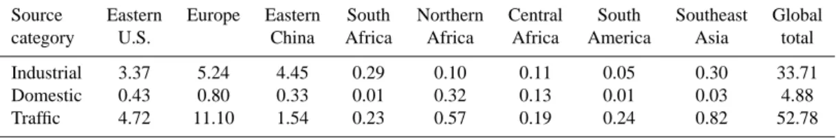
Table 1. Anthropogenic surface NOxemissions for the year 2000 assumed in this study.
Source Eastern Europe Eastern South Northern Central South Southeast Global category U.S. China Africa Africa Africa America Asia total Industrial 3.37 5.24 4.45 0.29 0.10 0.11 0.05 0.30 33.71 Domestic 0.43 0.80 0.33 0.01 0.32 0.13 0.01 0.03 4.88 Traffic 4.72 11.10 1.54 0.23 0.57 0.19 0.24 0.82 52.78 Values are given in Tg NO2/yr.
10:30 local time or hourly output; MATCH-MPIC and IM-AGES only provided monthly mean 10:30 local time data. For a proper comparison it is therefore useful to separate the models into two classes. The first (ensemble A) includes the CTMs that are driven by meteorology for the year 2000 and have provided daily (or hourly) data; the second (en-semble B) includes the CCMs and the GMI-DAO, MATCH-MPIC, and IMAGES CTMs. The nine A-ensemble mod-els (CHASER, CTM2, FRSGC/UCI, GEOS-CHEM, LMDz-INCA, MOZ2-GFDL, p-TOMCAT, TM4, and TM5) attempt to reproduce the measurements on a day-by-day basis; from the B-ensemble models we can only expect agreement in a time-averaged sense. The difference between the two ensem-bles will be clearly demonstrated when we discuss sampling issues in Sect. 5.3.
A description of the models’ characteristics and of the setup of the intercomparison simulations with focus on var-ious aspects important for tropospheric ozone is given by Stevenson et al. (2006). Here we will give a brief summary of the setup of the year-2000 simulations and treat some of the
issues related to tropospheric NO2in more detail. With the
exception of p-TOMCAT, all models included a reaction for
the hydrolysis of N2O5on aerosols (Dentener and Crutzen,
1993; Evans and Jacob, 2005). The reaction probability for this reaction varied between 0.01 and 0.1 (see Table A2).
Emissions of NOx, carbon monoxide (CO), non-methane
volatile organic compounds (NMVOCs), sulfur dioxide
(SO2), and ammonia (NH3)were specified on a 1◦×1◦grid.
To reduce the required spinup time of the near-future sce-nario simulations of the intercomparison study, the methane mixing ratios were specified throughout the model domain; for the year 2000 a global methane mixing ratio of 1760 ppbv was assumed. The anthropogenic emissions of the shorter-lived ozone precursor gases were based on national and regional estimates from the International Institute for Ap-plied Systems Analysis (IIASA) for the year 2000 (Co-fala et al., 2005; Dentener et al., 2005), distributed accord-ing to the Emission Database for Global Atmospheric Re-search (EDGAR) version 3.2 for the year 1995 (Olivier and Berdowski, 2001). Emissions from international shipping were added by extrapolating the EDGAR3.2 emissions for 1995, assuming a growth rate of 1.5% per year. The result-ing anthropogenic emissions were specified on a yearly
ba-sis, including separate source categories for agriculture (NH3
only), industry, the domestic sector, and traffic. The
corre-sponding emission totals for NOx are given in Table 1. In
some models (GMI, IMAGES, TM4, and TM5) the industrial emissions were released between 100–300 m above surface, using a recommended vertical profile; other models simply
added emissions to their lowest layer. For aircraft NOx
emis-sions a total of 2.58 Tg NO2(0.79 Tg N) was recommended
for the year 2000, with distributions from NASA (Isaksen et al., 1999) or ANCAT (Henderson et al., 1999).
Monthly emissions from biomass burning were specified based on the satellite-derived carbon emission estimates from the Global Fire Emissions Database (GFED) version 1 (van der Werf et al., 2003) averaged over the years 1997–2002, in combination with ecosystem dependent emission factors from Andreae and Merlet (2001). The corresponding yearly
total NOx emissions are given in Table 2. The main
rea-son for using the 1997–2002 average emissions is that the year-2000 simulations analyzed in this study served as the reference for the scenario simulations of the wider intercom-parison study on air quality and climate change. To eval-uate the impact of interannual variability in the emissions from biomass burning, we performed an additional simu-lation with the TM4 model using the GFED emissions for the year 2000 (see Sect. 5). Height profiles were specified for biomass burning emissions to account for fire-induced convection, based on a suggestion by D. Lavou´e (personal communication, 2004). These profiles were implemented by a subset of models (GMI, IMAGES, IMPACT,
MOZ2-GFDL, TM4, and TM5). In these models the emissions
from biomass burning were distributed over six layers from 0–100 m, 100–500 m, 500 m–1 km, 1–2 km, 2–3 km, and 3– 6 km. The biomass burning emissions are further described by Dentener et al. (2006c).
Recommendations were given for the natural emissions
of trace gases (Stevenson et al., 2006). For the NOx
emis-sions from soils, which represent natural sources augmented by the use of fertilizers, the models used values between 5.5 and 8.0 Tg N/yr. Another important but relatively uncertain
source is the NOxproduction by lightning (see Boersma et
al., 2005, and references therein), which varied between 3.0 and 7.0 Tg N/yr (see Table A2).
Table 2. NOxemissions from biomass burning from the Global Fire Emissions Database (GFED) averaged over the years 1997–2002 with
emission factors (EF) from Andreae and Merlet (2001), and for the year 2000 with the same emission factors or the updated values from M. O. Andreae (personal communication, 2004).
Inventory Eastern Europe Eastern South Northern Central South Southeast Global U.S. China Africa Africa Africa America Asia total GFED 1997–2002 0.07 0.09 0.02 0.27 7.21 6.86 3.76 0.94 33.14 GFED 2000 0.08 0.15 0.02 0.26 7.84 7.13 1.92 0.53 29.71 GFED 2000, updated EF 0.06 0.09 0.01 0.15 5.05 4.85 1.54 0.34 20.00 Values are given in Tg NO2/yr.
4 Method of comparison
In order to systematically compare models and retrievals, the
model NO2fields were analyzed at 10:30 local time and
col-located with the GOME measurements. This was done by sampling the local time model output at the locations of the scenes included in the BIRA/KNMI retrieval. In this re-trieval only forward-scan scenes with a cloud radiance
frac-tion lower than 0.5 for solar zenith angles smaller than 80◦
are included. The same selection criteria are applied in the Dalhousie/SAO retrieval. The retrieval by the Bremen group uses a slightly different selection based on a cloud fraction threshold of 20%. These differences imply that some incon-sistencies remain in the comparison of models with the Bre-men retrieval. Nevertheless, our collocation procedure cor-rects for most of the sampling bias of the retrievals resulting from incomplete spatial and temporal coverage of the satel-lite observations.
For the selected scenes, the modeled (sub)column density fields were linearly interpolated to the centre of the GOME ground pixels. As an intermediate step the data were mapped
onto a resolution of 0.5◦×0.5◦. The forward scans cover
an area of 320 km×40 km, which at the equator corresponds
to approximately 3◦×0.4◦; the horizontal resolution of the
models, on the other hand, ranges from 1◦×1◦ (TM5 over
zoom regions) to 22.5◦×10◦ (ULAQ), but is typically
be-tween 2◦and 5◦longitude/latitude. To eliminate the effect of
such resolution differences among the models and between models and retrievals, the model as well as the retrieval data
were smoothed to 5◦×5◦using a moving average.
The impact of collocating the model data with the
ob-servations is assessed by comparing the tropospheric NO2
columns from sampled and unsampled model output. (In the latter case the 10:30 local time column densities were
mapped directly onto a resolution of 0.5◦×0.5◦ and
there-after smoothed to 5◦×5◦.) In fact, by comparing the
sam-pled and unsamsam-pled model output, we can actually estimate the sampling biases in the monthly or yearly retrieval maps.
Such sampling biases are caused by temporal correlations
between the local cloud cover and the NO2column density.
In the annual mean this bias is to large extent determined
by seasonal variations, for instance in regions dominated by emissions from biomass burning. This seasonal contribution to the sampling bias can easily be removed by constructing a “corrected” annual mean by first calculating the monthly means and then averaging the monthly means. What remains is the contribution to the sampling bias resulting from day-to-day variability. To estimate this contribution, we removed the day-to-day variability in the 10:30 local time column output from the models by taking the monthly mean before sam-pling the data. The contribution from day-to-day variability to the sampling bias follows as the difference between the sampled daily and the sampled monthly fields.
In summary, the total sampling bias (SBtotal)in the
tropo-spheric NO2column density is given by
SBtotal=S(TCD(n)) − TCD(n),
where TCD(n) is the 10:30 local time tropospheric column density field on day n, the sampling operator S selects the scenes that have actually been retrieved, and the overbar de-notes a time averaging, per month or per year. The con-tribution from day-to-day variability to the sampling bias
(SBday−to−day)can then be expressed as
SBday−to−day=S(TCD(n)) − S(M(TCD(n))),
where the operator M assigns the monthly mean values to the daily fields. The remaining contribution related to seasonal
variations (SBseasonal)is thus given by the difference between
the sampled monthly fields and unsampled (monthly) fields:
SBseasonal =S(M(TCD(n))) − TCD(n)
=S(M(TCD(n))) − M(TCD(n)),
which vanishes in the monthly means, but is nonzero in the annual mean.
The corresponding expressions for the annual mean and
the corrected annual mean tropospheric NO2column density
are as follows:
annual mean = S(TCD(n))annual
corrected annual mean =DS(TCD(n))monthlyE
Here the overbar denotes the annual or monthly average and the brackets denote an averaging over the separate months weighted by the total number of days per month. Unless stated otherwise, the annual means presented in this study therefore always correspond to the unweighted averages over the individual scenes retrieved throughout the year.
Most models provided tropospheric NO2columns as
two-dimensional (2-D) fields assuming for the tropopause the level where the ozone mixing ratio equals 150 ppbv, as is done in the study by Stevenson et al. (2006). As the con-tributions from the upper troposphere and lower stratosphere are negligibly small compared to those from the lower and middle troposphere over polluted regions, the tropospheric
NO2 column density field is relatively insensitive to the
exact tropopause definition. Based on the 3-D 10:30
lo-cal time NO2 fields from the TM4 model, we estimate
that the assumption of a constant tropopause pressure of
200 hPa would change the annual mean tropospheric NO2
column density by an amount between –0.05 1015molecules
cm−2over tropical and subtropical continental regions and
+0.1×10¹⁵molecules cm−2at high latitudes.
Other models, including the three GMI models,
LMDz-INCA and p-TOMCAT, also provided 3-D NO2 fields at
10:30 local time. The availability of 3-D model output al-lows for a more direct comparison with the retrievals after
convolution of the modeled tropospheric NO2 profiles with
the averaging kernels of the retrievals. Application of aver-aging kernels makes the comparison independent of retrieval errors resulting from a priori profile assumptions (Eskes and Boersma, 2003). In this study the averaging kernels were taken from the BIRA/KNMI retrieval. The convolution was performed at the vertical resolution of the averaging kernels, having 35 layers in the vertical; 10:30 local time surface pressure fields from the European Centre for Medium Range Weather Forecasts (ECMWF) were used to regrid the model subcolumns in the vertical (see Sect. 5.4).
5 Results
5.1 Global maps for retrievals and models
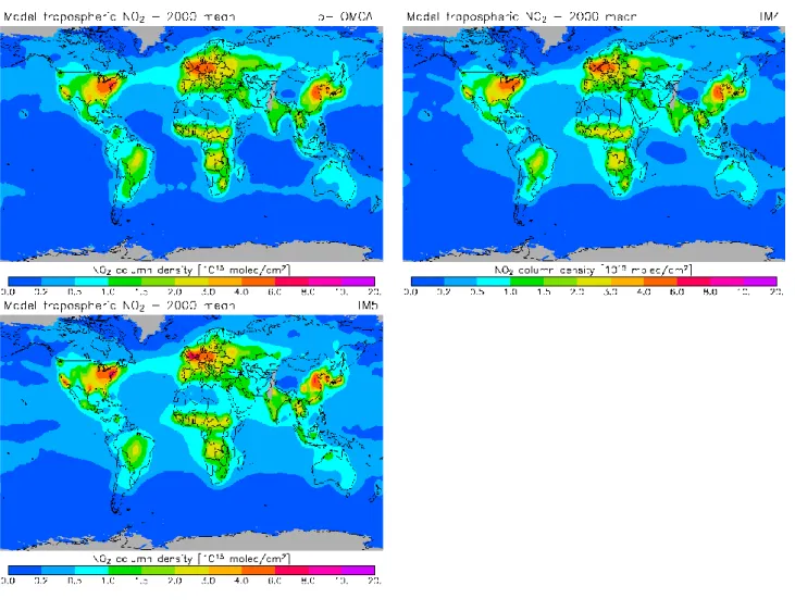
In Fig. 1 we present the annual mean NO2 columns from
the three retrievals for the year 2000. Shown are the
orig-inal retrieval data mapped to a resolution of 0.5◦×0.5◦ as
well as, for comparison with models, smoothed to 5◦×5◦.
The retrievals show qualitatively similar patterns of pollu-tion. Large-scale pollution is most pronounced over the east-ern United States, Europe, and easteast-ern China. High
tropo-spheric NO2 columns are also clearly observed over
Cali-fornia, South Korea, and Japan, as well as over the indus-trial Highveld region of South Africa. Enhanced levels of pollution are further seen over the Indian subcontinent, es-pecially over the Ganges valley in the north, around Delhi and Calcutta; over the Middle East, in particular around the
main ports of the Persian Gulf, around the Red Sea port of Jedda near Mecca, and around the cities of Riyadh, Cairo and Tehran; over the metropolitan cities of Mexico City, S˜ao Paolo/Rio de Janeiro, Buenos Aires, Moscow, Ekaterinburg, Chongqing (Central China), Hong Kong, and Sydney.
Rela-tively high tropospheric NO2columns are also observed over
the savanna regions of Northern Africa south of the Sahara and Central Africa south of the Equator; over the savanna, grassland and seasonally dry forest regions of South Amer-ica; and further over parts of Southeast Asia (Burma, Thai-land, Malaysia and the islands Sumatra and Java of the In-donesian archipelago). Relatively low values are observed over the oceans, over desert regions and other remote areas. These features are common to all three retrievals and remain
discernible after smoothing to 5◦×5◦.
The corresponding maps for the individual models of en-semble A and B are presented in Figs. 2 and 3, respectively. Shown are the 10:30 local time model output fields
collo-cated with the measurements and smoothed to 5◦×5◦. The
large-scale patterns observed in the retrievals are reproduced in a qualitative sense by the models. More localized pollution around main ports and metropolitan cities is at best partially resolved and is visible only in the higher-resolution models.
The spatial correlations between the annual mean
tropo-spheric NO2column density field of the individual models
and retrievals are given in Table 3. It demonstrates that the
smoothing to 5◦×5◦systematically improves the correlations
between models and retrievals, suggesting that the models do not accurately reproduce the small-scale features of the retrievals. Table 3 also shows that, even after smoothing, the observed patterns are better reproduced by the higher-resolution chemistry transport models of ensemble A than by the relatively coarse models of ensemble B. In particular the ULAQ model has difficulty representing the spatial
distribu-tion of the NO2column density, due to its coarse resolution
of 22.5◦×10◦.
The differences in model performance are caused by a complex interplay of various aspects of the chemistry and dynamics of the models. A comprehensive analysis of these factors is beyond the scope of this paper, but some of the differences can be explained in terms of differences in OH
levels, N2O5hydrolysis rates, and vertical mixing.
As estimated by Stevenson et al. (2006), the atmospheric
CH4lifetime in the models varies between 7.18 and 12.46
years (see Table A2). Since CH4is removed predominantly
by reaction with tropospheric OH, which was diagnosed in
the models even though the CH4 mixing ratio was fixed,
this indicates that there are rather large differences in OH among the models. Thus, the relatively low tropospheric
NO2 columns of the IMPACT, GMI-CCM and GMI-DAO
models might be explained if we assume that the NOx
life-time in these models is reduced due to high levels of OH,
corresponding to a low lifetime of CH4. Similarly, the high
CH4lifetime in CTM2 is consistent with the relatively high
Fig. 1. Annual mean tropospheric NO2column density from the three retrievals. Data are shown on a horizontal resolution of 0.5◦×0.5◦
(left) and smoothed to 5◦×5◦(right).
Other important factors determining the lifetime of NOx
are the reaction probability for hydrolysis of N2O5and the
description of the different types of aerosols. The models an-alyzed here typically include the hydrolysis reaction on
sul-fate aerosols with a reaction probability in the range 0.04– 0.1 (see Table A2). Evans and Jacob (2005) recently pro-posed a new parametrization for the reaction probability as a function of the local aerosol composition, temperature and
Table 3. Spatial correlation between the annual mean tropospheric NO2 column density field of the individual models and retrievals,
calculated at 0.5◦×0.5◦after smoothing the data to a common resolution of 5◦×5◦. The values in parentheses are the corresponding values calculated at 0.5◦×0.5◦before smoothing.
Region Global 50◦S–65◦N
Model/Retrieval BIRA/KNMI Bremen BIRA/KNMI Bremen Dalhousie/SAO GMI-CCM 0.88 (0.82) 0.81 (0.76) 0.89 (0.82) 0.85 (0.80) 0.86 (0.80) GMI-DAO 0.89 (0.82) 0.83 (0.78) 0.89 (0.82) 0.86 (0.81) 0.87 (0.81) GMI-GISS 0.88 (0.82) 0.84 (0.79) 0.88 (0.82) 0.87 (0.81) 0.86 (0.80) IMAGES 0.87 (0.80) 0.86 (0.80) 0.87 (0.80) 0.88 (0.82) 0.84 (0.78) IMPACT 0.87 (0.80) 0.84 (0.78) 0.87 (0.80) 0.86 (0.80) 0.82 (0.76) MATCH-MPIC 0.88 (0.81) 0.85 (0.79) 0.88 (0.81) 0.87 (0.81) 0.82 (0.76) NCAR 0.86 (0.80) 0.87 (0.81) 0.86 (0.79) 0.88 (0.83) 0.83 (0.77) ULAQ 0.79 (0.71) 0.79 (0.72) 0.77 (0.70) 0.80 (0.73) 0.75 (0.68) CHASER 0.91 (0.86) 0.90 (0.86) 0.90 (0.85) 0.92 (0.88) 0.85 (0.81) CTM2 0.89 (0.83) 0.89 (0.85) 0.88 (0.83) 0.90 (0.86) 0.83 (0.78) FRSGC/UCI 0.90 (0.85) 0.90 (0.86) 0.90 (0.85) 0.92 (0.88) 0.85 (0.80) GEOS-CHEM 0.91 (0.85) 0.88 (0.83) 0.91 (0.84) 0.90 (0.85) 0.87 (0.81) LMDz-INCA 0.90 (0.86) 0.91 (0.87) 0.90 (0.85) 0.93 (0.89) 0.87 (0.83) MOZ2-GFDL 0.91 (0.87) 0.91 (0.87) 0.91 (0.87) 0.92 (0.89) 0.86 (0.82) p-TOMCAT 0.92 (0.87) 0.92 (0.88) 0.91 (0.86) 0.93 (0.89) 0.88 (0.83) TM4 0.93 (0.89) 0.90 (0.87) 0.93 (0.89) 0.92 (0.89) 0.87 (0.84) TM5 0.92 (0.89) 0.90 (0.87) 0.92 (0.88) 0.92 (0.88) 0.86 (0.83)
relative humidity. This parametrization is included in the GEOS-CHEM model. The updated reaction probability has a global mean value of 0.02 and increases the tropospheric
NOx burden by 7%, compared to a simulation in which a
uniform value of 0.1 is assumed. The largest increases were found in winter, up to 50% at subtropical latitudes.
Vertical mixing is important mainly for two competing
reasons. On the one hand, the lifetime of NOx increases
with height. In summer it varies between several hours to a day in the lower troposphere and several days to a week in the upper troposphere. On the other hand, the daytime
NO2/NO ratio typically decreases by an order of
magni-tude from the surface to the upper troposphere, mainly
be-cause the reaction NO+O3→NO2progresses more slowly at
lower temperatures. For explaining the differences in
tro-pospheric NO2columns, the changes in the partitioning
be-tween NO2 and NO seem to be more important than the
changes in the lifetime of NOx. For instance, it has been
reported that the venting out of the boundary layer is too vig-orous in LMDz-INCA (Hauglustaine et al., 2004) (see also Sect. 5.4), which is consistent with the relatively low
tro-pospheric NO2columns simulated with this model. In
con-trast, the NCAR and MOZ2-GFDL models, which produce
relatively high NO2 columns, use a boundary layer mixing
scheme that tends to confine pollutants relatively strongly (Horowitz et al., 2003).
The NO2levels in the NCAR model may also be too high
because the conversion of organic nitrates and isoprene
ni-trates to NO2is too efficient. Other aspects of the chemical
and dynamical schemes as well as differences in deposition rates and natural emissions (see Table A2) may also be rele-vant.
5.2 Mean performance and uncertainties
Figure 4 displays the ensemble averages and the correspond-ing standard deviations for the three retrievals, for the full model ensemble, and for model ensemble A. For a proper comparison the 10:30 local time model output was collocated with the measurements, as was done in Figs. 2 and 3. More-over, retrieval and model averages and standard deviations
were calculated after smoothing the data to 5◦×5◦. The three
retrievals give significantly different NO2columns over the
continental source regions. Over the eastern United States and over eastern China the standard deviation among the
re-trievals goes up to about 1.5 and 2.0×10¹⁵molecules cm−2,
respectively. Larger differences are observed over South
Africa and Europe, where the standard deviation approaches
2.5 and 3.0×10¹⁵molecules cm−2, respectively. Except for
the Highveld region of South Africa, the major industrial re-gions are much less polluted in the Dalhousie/SAO retrieval than in the BIRA/KNMI and Bremen retrievals (see Fig. 1). For the model ensemble we find comparable standard de-viations over the eastern United States, Europe and eastern
China – up to 2.0×10¹⁵molecules cm−2for the full
ensem-ble and up to 1.5×10¹⁵molecules cm−2 for ensemble A.
Over India and northeastern Australia the models also show a smaller spread than the retrievals; the reverse is observed over Central Africa south of the Equator.
Fig. 2. Annual mean tropospheric NO2column density for the A-ensemble models. Data have been smoothed to a horizontal resolution of
5◦×5◦.
Note that the standard deviation among the A-ensemble models is generally significantly smaller than for the full model ensemble. The ensemble averages on the other hand are very similar, indicating that the use of climate models introduced random errors. This similarity is demonstrated
more clearly in Fig. 5, which shows the difference between the model ensemble averages and the retrieval average. The full ensemble produces a more diffuse pattern than the re-stricted A ensemble, resulting in slightly higher values over oceans and remote regions; over polluted regions, the two
Fig. 2. Continued.
ensembles give nearly identical average values. On aver-age the models underestimate the retrievals in industrial re-gions and overestimate the retrievals in rere-gions dominated by biomass burning. By far the strongest underestimation of up
to 6.0×10¹⁵molecules cm−2 is found over the Bejing area
of eastern China. Over the Highveld region of South Africa as well over Western Europe south of Scandinavia the
mod-els underestimate the retrievals by up to 4.0×10¹⁵molecules
cm−2. Smaller underestimations are found over the other
industrial regions mentioned in Sect. 5.1, in particular over the eastern United States, California, the Persian Gulf, India, Hong Kong, South Korea and Japan. The models are also
un-able to reproduce the relatively high NO2columns over the
southwest of Canada. The strongest overestimations (up to
1.5×10¹⁵ molecules cm−2)are found over the savanna
re-gions of Brazil south of the Amazon basin and over Angola. The models further overestimate the retrievals over Zambia and the southern Congo, over the south coast of West Africa, over the Central African Republic and southern Sudan, as well as over Southeast Asia. Simulated columns are also
higher than retrieved over the North Atlantic, Ireland, Scot-land, Scandinavia and the Baltic States.
5.3 Sampling bias
Figure 6 shows the annual mean bias distribution resulting from incomplete spatial and temporal coverage of the GOME measurements, as estimated from the models. As a proxy for the actual sampling bias of the retrievals, we have calculated the difference between the sampled and unsampled 10:30 lo-cal time output from the models. The best estimate of the sampling bias is derived on the basis of the A-ensemble; the corresponding result for the B-ensemble models can only ac-count for part of the actual sampling bias, as will be demon-strated below.
Both ensembles consistently indicate that the satellite products are positively biased over the large biomass burn-ing regions of Africa (up to 48%), South America (up to 38%), and parts of Southeast Asia, including Burma, Laos and Thailand (up to 28%). The sampling biases over these regions are related to the fact that there are relatively few
Fig. 3. Annual mean tropospheric NO2column density for the B-ensemble models. Data have been smoothed to a horizontal resolution of
Fig. 4. Ensemble average annual mean tropospheric NO2 column density with corresponding standard deviation for the three GOME
retrievals, the full model ensemble (A+B), and ensemble A separately. These quantities have been calculated after smoothing the data to a horizontal resolution of 5◦×5◦.
observations during the wet seasons due to the presence of clouds; the annual means are therefore biased towards the high column values observed during the dry burning season.
Relatively small positive biases are found over the north of Canada, over northern Kazakhstan, and over eastern Siberia. Because of the similarity of the bias patterns generated by the
Fig. 5. Annual mean tropospheric NO2column density difference between models and retrievals for the full model ensemble (A+B) and
ensemble A separately. Data have been smoothed to a horizontal resolution of 5◦×5◦.
Fig. 6. Total sampling bias for ensembles A and B. Data have been smoothed to a horizontal resolution of 5◦×5◦.
two ensembles, these biases must also be caused by correla-tions on seasonal time scales between local cloud or snow
cover and tropospheric NO2column density.
Negative biases are observed over the eastern United States, Europe, and eastern China. In these regions, the two ensembles give rather different results, however. Our best estimates based on the A-ensemble models indicate
nega-tive biases down to –1.7×10¹⁵molecules cm−2(–47%) over
Europe, –1.5×10¹⁵molecules cm−2 (–34%) over the
east-ern United States, and –0.8×10¹⁵molecules cm−2 (–21%)
over eastern China. The B-ensemble models would result in significantly smaller bias estimates in these regions,
be-cause the tropospheric NO2columns from these models do
not reflect the synoptic-scale meteorological variability of the year 2000. The ensemble-A models, on the other hand, do account for day-to-day fluctuations related to
meteorolog-ical conditions. The contribution of day-to-day variability to the sampling was calculated as described in Sect. 4. Fig-ure 7 shows that this contribution is very different for the two sets of models. For the B-ensemble models we find a negligible contribution from day-to-day correlations (time scales shorter than a month); for this set of models the sam-pling biases shown in Fig. 6 are therefore almost entirely re-lated to correlations on seasonal time scales. This is not the case for the A-ensemble models, where day-to-day correla-tions do give rise to an additional contribution to the sam-pling bias. In fact, the day-to-day samsam-pling bias is as large –
1.0×10¹⁵molecules cm−2over the eastern United States and
in the range –0.7 to +0.4×10¹⁵molecules cm−2 over
east-ern China, and accounts for most of the sampling bias over these regions. There is also a significant impact over Europe,
Fig. 7. Contribution of day-to-day variability to the sampling bias for ensembles A and B. Here the B-ensemble mean does not include the
MATCH-MPIC and IMAGES models, which provided only monthly output. Data have been smoothed to a horizontal resolution of 5◦×5◦.
cm−2 are found over Scandinavia and Central Europe and
positive contributions up to 0.5×10¹⁵molecules cm−2over
Western Europe.
It should be emphasized that these numbers are estimates based on model assumptions and that in reality a different bias could exist. The impact of clouds, for example, could
be quite different depending on the vertical profile of NO2,
which in turn depends on the vertical mixing and vertical emission profile used in the models.
Note also that our definition of the sampling bias does not account for differences between the 10:30 local time and
the 24-h average tropospheric NO2 column density. From
a simulation of the TM4 model with diurnally varying an-thropogenic emissions in Europe (see Sect. 6.2), we estimate that the 10:30 local time columns over this region are 71.7% (February) to 55.9% (October) – or 65.6% in the corrected annual mean – of the corresponding diurnal average values. Similar ratios were reported by Velders et al. (2001). For
the comparison with NO2 retrievals from space it is
there-fore essential to consider only model output at or close to the overpass time of the satellite.
5.4 Averaging kernels
The results presented above have all been obtained on the basis of the 2-D output fields from the model. In this sec-tion we will test the sensitivity of the results to the appli-cation of averaging kernels. Three models from ensemble
A provided 10:30 local time 3-D NO2fields: LMDz-INCA,
p-TOMCAT and TM4. In Fig. 8 we present for these mod-els the tropospheric column density maps obtained by con-volution of the collocated data with the averaging kernels of the BIRA/KNMI retrieval. Also shown in Fig. 8 are the differences between these maps and the corresponding maps derived from the 2-D model output fields (shown earlier in
Fig. 2). LMDz-INCA and p-TOMCAT exhibit similar pat-terns of sensitivity over industrial regions. For these mod-els the application of the averaging kernmod-els leads to an
in-crease of up to 1.5×10¹⁵molecules cm−2over eastern China
and up to 1.0×10¹⁵molecules cm−2 over the northeastern
United States and over Europe. These increases imply that
the vertical tropospheric NO2profile in these regions is not
as steeply decreasing with height in the LMDz-INCA and p-TOMCAT models as does the a priori profile assumed in the BIRA/KNMI retrieval.
TM4 shows a much less sensitive response in these re-gions, which can be understood from the fact that the a priori profile used in the BIRA/KNMI retrieval is actually based on the TM4 model. Nevertheless the application of the averag-ing kernels does have a nonzero impact in large parts of the world even for the TM4 model. This is related to the fact the retrieval has used another version of the model with differ-ent emissions from anthropogenic sources and from biomass burning; moreover, in the current version of the model the biomass burning emissions are also distributed as a function of height, as described in Sect. 3. Indeed the TM4 model is most sensitive to the application of the averaging kernels over the biomass burning regions of Africa. Here the response pattern is similar for the three models with increases of over southern Sudan, the Central African Republic and the south-ern Congo, and decreases over Angola and Zambia, as well as over the south coast of West Africa.
Increases are found where the model profile is flatter than the a priori profile and can be explained by the height distri-bution of the biomass burning emissions in the TM4 model simulation; decreases are related to differences between the Global Fire Emissions Database (GFED) emissions assumed in this intercomparison study and the biomass burning emis-sion inventory assumed in the TM4 model veremis-sion used in
Fig. 8. Annual mean tropospheric NO2column density calculated by application of the averaging kernels to the daily 3-dimensional output fields from the three A-ensemble models LMDz-INCA, p-TOMCAT and TM4 (left). The difference compared to the corresponding fields shown in Fig. 2, which were obtained directly from the daily model columns, is shown in the panel on the right. Results for the TM4 model in an alternative setup in which all biomass burning emissions (BBE) are released below 100 m, are included as well. Data have been smoothed to a horizontal resolution of 5◦×5◦.
the retrieval (estimates for the year 1997 from the European Union project POET). To demonstrate the validity of this argument, we performed an additional simulation with the TM4 model following the setup of Sect. 3, but with all emis-sions from biomass burning released near the surface (below 100 m). Over the biomass burning regions the response to the application of the averaging kernels changes in line with the explanation given above: with biomass burning emissions released near the surface, the regions of positive impact in Africa have disappeared and the regions of negative impact have extended significantly (Fig. 8).
The application of the averaging kernels yields a closer agreement between the LMDz-INCA and p-TOMCAT mod-els with the BIRA/KNMI retrieval over the large parts of the industrialized world. However, averaging kernels are at best part of the explanation for the observed discrepancy between models and retrievals: the inclusion of profile information from the models removes only a fraction of the
underestima-tion by the models of the retrieved columns over industrial regions and may even lead to enhanced discrepancies over some of the biomass burning regions. Since the response is determined by local differences between the a priori profile assumed in the retrieval and the corresponding profile from the model, details of the response pattern may be quite dif-ferent for the other models. Moreover, it should be realized that the averaging kernels used in this study allow for a more direct comparison with the BIRA/KNMI retrieval only.
5.5 Regional analysis
The seasonal cycle in tropospheric NO2from models and
trievals was analyzed in more detail for eight continental re-gions of relatively high pollution (see Fig. 9). These include industrial regions (the eastern United States, Europe, eastern China and South Africa) as well as the regions dominated by emissions from biomass burning (Northern Africa, Central
Fig. 8. Continued.
Africa, South America and Southeast Asia). For these re-gions we calculated the monthly and yearly average
tropo-spheric NO2column densities from the retrievals and from
the collocated 10:30 local time model output, thus focusing on differences not related to sampling issues. In Fig. 10 the seasonal cycle obtained with the A-ensemble models is com-pared with the retrievals. The left panel shows the monthly mean values derived from the 2-D model output; the right panel shows the corresponding values obtained by applica-tion of the averaging kernels to the 3-D output from LMDz-INCA, p-TOMCAT and TM4, together with the retrieved monthly means.
As shown previously, over the industrial regions the spread in absolute column abundances is generally larger among the retrievals than among the A-ensemble models (see Fig. 4) and on average the models tend to underestimate the re-trieved values (see Fig. 5). From the seasonal cycles shown in Fig. 10, it can be observed that the differences among the retrievals are particularly pronounced in wintertime; more-over, it can be seen that the ensemble average discrepancy between models and retrievals is dominated by the fact that
the models do not reproduce the highest wintertime values produced by the retrievals.
Following the argument of Sect. 5.1, this might indicate that many of the boundary layer schemes used in the models have difficulty suppressing the vertical mixing under stable conditions. Possibly the models also tend to overestimate the
N2O5hydrolysis reaction rate. According to Evans and
Ja-cob (2005), the assumption of a uniform reaction probability
of 0.1 would lead to an underestimation of the NOx
concen-trations by up to 50% in wintertime. However, even the mod-els with lower reaction probabilities as well as the GEOS-CHEM model, in which the parametrization of Evans and Jacob (2005) is applied, are unable to reproduce the strong wintertime enhancement seen in the European retrievals over industrial regions.
The discrepancy between models and retrievals is particu-larly pronounced over eastern China. The most likely expla-nation is that the IIASA/EDGAR3.2 inventory significantly underestimates the emissions from eastern China, especially in wintertime. Kunhikrishnan et al. (2004a) performed sim-ulations with the MATCH-MPIC model using anthropogenic