HAL Id: halshs-00196084
https://halshs.archives-ouvertes.fr/halshs-00196084
Submitted on 12 Dec 2007
HAL is a multi-disciplinary open access
archive for the deposit and dissemination of
sci-entific research documents, whether they are
pub-lished or not. The documents may come from
teaching and research institutions in France or
abroad, or from public or private research centers.
L’archive ouverte pluridisciplinaire HAL, est
destinée au dépôt et à la diffusion de documents
scientifiques de niveau recherche, publiés ou non,
émanant des établissements d’enseignement et de
recherche français ou étrangers, des laboratoires
publics ou privés.
Endogenous persistent inequality
Falilou Fall
To cite this version:
Maison des Sciences Économiques, 106-112 boulevard de L'Hôpital, 75647 Paris Cedex 13
http://mse.univ-paris1.fr/Publicat.htm
Equipe Universitaire de Recherche
en Economie Quantitative - UMR 8594
Endogenous persistent inequality
Falilou FALL, EUREQua
Endogenous Persistent Inequality
1.Falilou FALL
2Université Paris 1 Panthéon-Sorbonne, EUREQua
October 4, 2005
Keywords: Endogenous Inequality, Human Capital, Occupational Choice, Education JEL Classi…cation: J24, J62, J31, D33
1I am grateful to H. d’Albis, A. d’Autume, B. Decreuse, D. de la Croix, J.-P. Drugeon, E. H. Fall, J.-O. Hairault, C. Le Van,
Y. Nyarko, T. Piketty, J.-V. Ríos-Rull, A.Venditti and B. Wigniolle for helpful suggestions and seminar participants at PSE-Jourdan, EUREQua, GREQAM, T2M, EALE/SOLE conference, PET 05 and Vigo X Dynamic Macroeconomics Workshop for their comments. The usual disclaimer applies.
2Université Paris 1, Maison des Sciences Economiques, EUREQua, 106-112 boulevard de l’Hôpital, 75647 Paris cedex 13,
Abstract
The purpose of this paper is to demonstrate that inherited human capital is a powerful vector of inequality formation and persistence, irrespective of its links with …nancial wealth endowment. This paper argues that the agents who inherit a low level of human capital bear a greater utility cost in their educational investment and that there are di¤erent pro…les of returns on human capital within the economy. These two arguments are su¢ cient to generate an endogenous formation of workers’and entrepreneurs’groups and a continuum of steady states with inequality. Allowing for self-employment in the model generates the possibility of equality at equilibrium in addition to the inequality equilibrium with the emergence of a middle class.
Keywords: Endogenous Inequality, Human Capital, Occupational Choice, Education JEL Classi…cation: J24, J62, J31, D33
Résumé
Dans ce papier, nous montrons que le capital humain hérité est un puissant vecteur de formation et de persistance des inégalités qui ne dépend pas de la richesse …nancière reçue. Nous défendons que les agents qui héritent d’un niveau de capital humain faible supportent un coût en utilité plus grand dans leur investissement éducatif et qu’ils existent di¤érents pro…ls de rendement du capital dans l’économie. Ces deux arguments sont su¢ sants pour générer une formation endogène des groupes de travailleurs et entrepreneurs et un continuum d’états stationnaires avec inégalités. Lorsqu’on permet aux agents d’être des entrepreneurs individuels alors le modèle génère la possibilité d’un équilibre avec égalité en plus de l’équilibre avec inégalités. Dans le cas d’un équilibre inégalitaire, une classe moyenne émerge comme une opportunité d’échapper au marché du travail pour les agents qui ont hérité d’un capital humain moyen.
1
INTRODUCTION
A central prediction of modern macroeconomic theories is that wealth distribution (and its transmission) is a key factor of inequality formation and persistence. Although the literature on the consequences of intergen-erational links on income and wealth distribution is vast, it can be split into two groups. In the …rst group, the mechanism generating inequalities depends on agents’ investment opportunities, given their inherited wealth, with human capital playing no role. Among others we can cite Aghion and Bolton [1997], Banerjee and Newman [1993], Piketty [1997], Matsuyama [2000] and Ghatak and Jiang [2001]. In the second group, human capital accumulation or investment is the central mechanism that determines agents’opportunities and occupations and therefore inequality in the economy. Since Loury’s [1981] seminal contribution, this …eld has received many contributions, these of Galor and Zeira [1993], Ljungqvist [1993], Durlauf [1996] and Mookherjee and Ray [2003] among many others.
This literature3 emphasizes the role of wealth distribution, imperfect capital markets and non convexities in order to exhibit the persistence of inequalities and the long-run e¤ects of the initial distribution. Imperfect credit markets prevent less endowed agents from borrowing and prevent them from having access to high levels of education or investment. It limits their ability to get involved in an entrepreneurial activity or high return investment. Therefore inherited …nancial wealth fully determines agents’and family occupations and paths.
Since the important contribution of Lucas [1988], it has been admitted that human capital is a central engine of economic growth. Galor and Tsiddon [1997] show that the distribution of human capital is a key factor in the determination of the pattern of economic development and income distribution. They show that when the e¤ects of parental human capital dominate the average level of human capital in the process of human capital accumulation, then the distribution of income becomes polarized in the long run. In this vein, Durlauf [1996] shows that parents a¤ect their children’s income through the choice of a neighborhood in which to live. Their model exhibits endogenous strati…cation, since wealthier families have strong incentives to segregate themselves into economically homogeneous neighborhoods.
The role of human capital in the formation and persistence of inequalities is largely supported by empirical evidence. Among many others, Becker and Tomes [1979], [1986] stress that the income of children is raised when they receive more human capital from their parents. They also show that the family endowments, namely, genetically determined race, ability, family reputation and connections, knowledge, skills and goals are a strong vector of inequality transmission. Moreover, Dunn and Holtz-Eakin [2000] state that parents a¤ect the entrepreneurship decisions of their children through human capital more than through …nancial means.
A critical aspect of these models is that human capital is closely linked with …nancial wealth in the mechanism which generates inequality formation and persistence. One may wonder whether there exists a fundamental mechanism of inequality formation and persistence which rests on the interplay between the human capital distribution and the labor market.
3An exception is Chatterjee [1994] who showed that in a neoclassical framework, with the assumption of a perfect market,
The purpose of this paper is to demonstrate that inherited human capital is a powerful vector of inequality formation and persistence, irrespective of its links with wealth endowment. The distribution of human capital determines the structure of occupations in the economy, the relative returns on occupations and the distribution of agents into these occupations. The importance of such mechanisms is to highlight the complementarity of human capital and …nancial wealth in explaining agents’and family trajectories. That is, agents’ choices of human capital investment, and therefore occupations, does not depend only on their wealth and borrowing capacity, but also on the opportunity their inherited level of human capital o¤ers to them. This opportunity depends on the entire distribution of human capital.
With this aim, we build an overlapping generations model. Individuals are identical in their preferences and their human capital production technology. However, they may di¤er in the level of human capital they inherit from their parents. Agents make two decisions as follows. First, they decide upon the time they devote to education when they are young. Secondly, when they are adult, they decide upon whether their occupation will be that of entrepreneur or worker. The key features of the model are that the agents who inherit a low level of human capital4 bear a greater utility cost in their education investment, and that
there are di¤erent pro…les of returns on human capital within the economy. Therefore, agents have di¤erent comparative advantages in their educational investment and their occupational choice, given their inherited level of human capital.
We …rst show that there exists a unique human capital threshold which separates agents into workers and entrepreneurs. This human capital threshold is endogenously determined as it depends on the equilib-rium wage. Agents whose inherited human capital is lower than the human capital threshold are better o¤ becoming workers, while those whose inherited human capital is greater are better o¤ becoming entrepre-neurs. Therefore, the inherited level of human capital, and especially its relative position in the distribution of human capital, are determinant in an agent’s occupational choice. We also show that di¤erent levels of investment in education are associated with these occupations. In particular, workers invest less in education than entrepreneurs, thereby magnifying inequality.
These di¤erent occupations, implying inequality in the utility and in the human capital level, persist in the long run. The model exhibits a two-point distribution of human capital and income at every steady state. In other words, the population is polarized into the rich entrepreneurs whose revenue is decreasing with the equilibrium wage and the poor workers whose revenue is increasing with the equilibrium wage. This magni…es the labor con‡ict between workers and entrepreneurs. It is also shown that economies with di¤erent initial human capital distributions converge to di¤erent levels of steady state inequality, both in terms of the number of agents in each type of occupation and of equilibrium wage. In short, the model exhibits a continuum of steady states with inequality. That is, for any possible initial distribution of human capital there exists a continuum of steady states with inequality to which it can converge. However, this continuum of steady states is bounded in terms of number of agents in each occupation, independently of the initial distribution of human capital. Mookherjee and Ray [2003] have shown that the outcome of a continuum of steady states is chronic whenever the number of occupations in the economy is small.
4The concept of human capital retained is general. It may include the di¤erent demensions of human capital: cognitive
Among these steady states equilibria, there exists one which maximizes social welfare, in the sense of the sum of agents’indirect utility. It is therefore possible to design a redistributive permanent policy in order to implement a better steady state equilibrium in terms of the mean utility of agents. It is worth noting that redistributive policy in this context does not change the initial distribution of human capital, but it a¤ects the incentives agents have in their occupational choice. Moreover, the group of agents to tax and the group to subsidize depends on the distribution of human capital. For some distribution of human capital, it becomes preferable to tax workers’revenues and to subsidize entrepreneurs’revenues in order to increase the fraction of entrepreneurs, both in the short run and at the steady state in order to obtain a greater mean utility in the economy.
Extending the model to allow for self-employment generates two alternative types of equilibrium. In one case, all agents are self-employed entrepreneurs, and make the same investment in education. In the long run, those agents have the same human capital level and earn the same income. Mookherjee and Ray [2003] argue that inequality is inevitable because of the pecuniary externalities that induce the population to sort itself into di¤erent occupations with unequal net incomes. However, here the possibility of self-employment creates the condition for some distribution to break the inescapable character of inequality. Inequality disappears at the steady state.
In the other case, agents are split up across the three occupations: workers, self-employed entrepreneurs and employer-entrepreneurs. The long-run distribution of human capital is then a three-point distribution, magnifying status and income inequalities between agents. Which of these two alternative scenarii will be realized crucially depends on the initial human capital distribution. For instance, if the distance between the low and the high level of human capital in the economy is large and if the agents’ allocations are uniformly distributed, it is likely that the economy will develop a three occupations equilibrium. In that case, the opportunity for self-employment generates a middle class of agents. The human capital level of these middle-class agents is high enough to allow them to be better o¤ working for themselves. This possibility of self-employment bene…ts agents who are relatively weakly endowed in human capital more, since they gain the opportunity to escape from the labor contract. Therefore, the model explains the emergence of a professional class (lawyers, doctors etc.) as an intermediate opportunity for agents who receive a relatively middle level of human capital.
In the literature5 of the impact of human capital distribution on occupational structure and inequality, the contribution of Banerjee and Newman [1993] and Matsuyama [2003] are the most closely related to ours. In these papers, the vertical division of labor and wealth distribution play a central role. Banerjee and Newman’s [1993] main concern is historical dependence, which is yielded by the non-convex investment technology. Matsuyama [2003] analyzes the e¤ects of wealth distribution on occupational structure through the imperfect credit market. The approach of this paper is di¤erent. First, we consider that the credit market is perfect and there is no borrowing limit in the economy. Secondly, there are no barriers to becoming an entrepreneur, that is, there is no non-convexity in the investment technology although, the model exhibits non-convexities in the occupational structure.
5Other studies in this literature of long run distribution considering the labor market contract or human capital include
The plan is as follows. In section 2 we set up the model and derive the endogenous human capital occupational threshold. In section 3 we discuss the existence and uniqueness of short run equilibrium. In section 4, we analyze the persistence of inequalities in the long run and the steady states equilibria. In section 5, we study the redistributive policy. In sections 6 and 7, we introduce the possibility of self-employment and analyze the di¤erent types of equilibria that emerge. Section 8 concludes.
2
THE MODEL
The framework is a two-period OLG model with human capital intergenerational transmission within families. Each agent lives two periods. The only source of heterogeneity within a group of same-aged individuals is their human capital inheritance. To simplify the exposition of the model we do not consider the …nancial capital. We can do so because we assume that capital markets are perfect and there is no market imperfection in the economy. The absence of capital variable does not change the qualitative results of the model. Indeed, should we add a capital factor in the production function, either of the good or of human capital, agents’ decisions would not be altered.
2.1
Entrepreneurship
An entrepreneur faces the following technology
Yit+1= hit+1Lit+1 (1)
where 0 < ; < 1 and + > 1 , where hit+1 is the human capital of the entrepreneurs (the owner of
the business) and Lit+1 is the total e¤ective labor factor hired by the entrepreneur. Lit+1 is the sum of
the e¢ cient unit of human capital of the workers. As we abstract from the capital variable, there is only one explicit market6 in this economy: the labor market which determines the equilibrium wage per unit of human capital and therefore workers’ earnings. The entrepreneur’s human capital re‡ects her managerial ability and therefore the size of the business she can run. The entrepreneur’s revenue is the pro…t from her business and it depends on the size of the latter. The assumption of increasing returns to scale plays an important role. Indeed, it implies that at the aggregate level the pro…le of entrepreneurs’earnings is convex and increases with human capital. This creates the break between the workers’and entrepreneurs’earnings pro…le.
The pro…t maximizing program of an entrepreneur is therefore max
Lit+1
h
hit+1Lit+1 wt+1Lit+1
i
Solving this problem yields the optimal labor demand of the entrepreneur depending on her proper level of human capital: Lit+1= hit+1 wt+1 ! 1 1 (2)
Therefore the entrepreneur’s pro…ts or earnings are written:
i(hit+1) = hit+11 w t+1
1
(1 ) (3)
The convexity of i(hit+1) implies that there is no one optimal level of production and pro…t in the economy,
but that for any given level of entrepreneurial human capital there is only one optimal level of production and pro…t. Thus there is no constraint on setting up an entrepreneurial project, but entrepreneurs will di¤er in the size of the business they can run and therefore in their earnings. Therefore, there is a continuum of enterprises that can exist in this model, depending on the distribution of human capital.
2.2
Agents’ occupational choice
In her youth, every agent receives a human capital hitfrom her parents and an endowment of one unit of time.
She then allocates her time between training in education (uit), and leisure (lit= 1 uit). The time invested
in education determines her second period level of human capital hit+1. When adult, the agent chooses either
to become a worker or to become an entrepreneur-manager. If she chooses to be an entrepreneur-manager she will earn at the end of the period the pro…t (hit+1) from running the business. If she chooses to be a
worker, she will earn wt+1hit+1where wt+1is the equilibrium wage per unit of e¢ cient human capital. The
agent consumes all her revenue before leaving the economy. The agent utility function depends on her …rst period leisure litand her second period consumption cit+1. For simplicity, we do not consider consumption7
in the …rst period, and we assume that agents inherit human capital from their parents. The agent’s program is written: M ax lit;cit+1 U (lit; cit+1) = l1it cit+1 (4) s:t: 8 > > > > > < > > > > > : lit+ uit= 1 hit+1= (uithit) cit+1= yit+1
yit+1= max fwt+1hit+1, (hit+1)g
where 0 < < 1 and > 0 represents the e¢ cacy of the educational system or human capital transmission from parents to child. This program is not di¤erentiable on one point, but continuous. Thus, local solutions on both sides of the non-di¤erentiable point are both global solutions.
From an agent’s perspective, the occupational choice is a maximizing of indirect utility function. The agent chooses to become an entrepreneur if her indirect utility of becoming an entrepreneur, let us denote it VE(hit; wt+1), is greater than her indirect utility of becoming a worker VW(hit; wt+1). Therefore to solve
the global program of the agent, one can compute the two distinct indirect utility functions of becoming an entrepreneur or a worker. The program of the entrepreneur is written:
7For exemple Glomm and Ravikumar [1992] make the same simplifying assumption on …rst period consumption. Adding
M ax lit;cit+1 U (lit; cit+1) = l1it cit+1 s:t: 8 < : lit+ uit= 1 cit+1= 1 (uithit)1 wt+1 1 (1 ) Solving this program gives her optimal time investment in education:
uEit =
(1 ) (1 ) + (5)
and her second period human capital: hEit+1=
(1 ) (1 ) + hit (6)
The optimal corresponding indirect utility function of an entrepreneur is :
VE(hit; wt+1) = (1 ) 1 (1 ) (1 ) (1 ) (1 ) + 1 (1 ) (1 ) + 1 wt+1 1 h1 it (7) The program of a worker is written:
M ax lit;cit+1 U (lit; cit+1) = lit1 cit+1 s:t: 8 < : lit+ uit= 1 cit+1= wt+1 (uithit)
her optimal time investment in education is: uWit =
1 + (8)
and, therefore her second period human capital is: hWit+1=
1 + hit: (9)
The optimal corresponding indirect utility function of a worker is: VW(hit; wt+1) =
1 1 +
1
1 + wt+1hit : (10) Due to the assumption of concavity and the Cobb-Douglass form of both the utility function and the production function of the human capital, the time investment in training is independent of agents’ levels of human capital and of the expected wage as given by equations (5) and (8). That is, all entrepreneurs-managers devote the same time to training even if they do not have the same level of human capital. Likewise, all workers invest the same amount of time in training. Moreover, entrepreneur-managers invest a greater
amount of time in training than workers. Because entrepreneur-managers inherit a greater level of human capital, they have a lower disutility or opportunity cost in investing a higher level of human capital.
As seen in equations (6) and (9) the second period level of human capital of agents is independent of the expected equilibrium wage. This feature of the human capital transition equation has important implications for the dynamics of the economy and of the human capital.
Agents’indirect utility function is an increasing function of their inherited human capital. But while it is increasing with the equilibrium wage for the workers, it is decreasing with the equilibrium wage for the entrepreneurs.
2.3
Human capital occupational threshold
Given the distribution of human capital, what will be the cut-o¤ point between being workers and being en-trepreneurs? Let us consider V (hi; wt+1) VW(hi; wt+1) VE(hi; wt+1). For each agent, when V (hi; wt+1)
is positive she chooses to be a worker, if it is negative she chooses to be an entrepreneur. At the macro-economic level we show that there is a unique human capital level that separates the group of workers and the group of entrepreneurs. As illustrated by Figure 1, for a given wage the function V (hi; wt+1) is positive
for all hi< ~hit and is negative for all hi> ~hit. There is a unique positive level of human capital for which
V (hi; wt+1) = 0. For that level of human capital, denoted the human capital occupational threshold, agents
are indi¤erent8 between being workers or entrepreneurs.
Figure 1: Human Capital Occupational Threshold
Proposition 1 : There is a unique human capital threshold depending on the equilibrium wage that separates workers from entrepreneurs.
Proof. Since for a given wage wt+1 V"(hi; wt+1) < 0 then, V (hi; wt+1) is strictly concave, and as
V (0) = 0 and limhi!1V (hi; wt+1) = 1; there exists a unique and positive human capital level ehi; for
which V ehi; wt+1 = 0. Thus for any hi< ehi, V (hi; wt+1) > 0 and agents choose to become workers while,
for all hi> ehi; V (hi; wt+1) < 0 and agents choose to become entrepreneurs.
Equalizing Vw(h
i; wt+1) = VE(hi; wt+1) gives the occupational threshold ehit. It is written:
~ hit(wt+1) = [(1 ) (1 ) + ] (1 + ) (1 ) (1 )(1 ) ( + 1) (1 ) (1 ) + ( + 1) (11) 11 1 + 1 ( + 1) 1 ( + 1) 1 1 1 ( + 1) (wt+1) 1 ( + 1)
This occupational threshold ~hit(wt+1) increases with the equilibrium wage. Indeed when the equilibrium
wage is high, more agents are better o¤ becoming workers than entrepreneurs. A higher equilibrium wage per unit of human capital implies more earnings for workers and lower pro…ts for entrepreneurs, whereas a low level of the equilibrium wage lessens the labor cost, which leads to a lower level of human capital becomeing pro…table when employed in an entrepreneurial activity. This implies a low level of occupational threshold. Now we turn to the general equilibrium of this model.
3
SHORT-RUN EQUILIBRIUM
Since agents only work during their second period of life, contracts in markets are agreed by agents from the same generations. This implies that the next period expected equilibrium wage is known today, as it is completely determined by the choices made by today’s generation of agents. Therefore we write the equilibrium of the model by solving the next period market.
Let (hi); with values in (0; 1), denote the distribution function of human capital across agents, where
hiis de…ned in R+between hmini and hmaxi . The short run equilibrium of the economy is de…ned by the joint
determination of the equilibrium wage that regulates the competitive labor market and the human capital occupational threshold at any date t. The labor market is competitive in the sense that at any date there is an equilibrium wage per unit of human capital which equalizes labor supply and labor demand. Therefore, the equilibrium condition of the labor market is written:
1 + Z h~it(wt+1) hmin it hitd t(hi) = wt+1 1 1 1 (1 ) (1 ) + 1 Z hmaxit ~ hit(wt+1) h1 it d t(hi) (12) The left hand side of equation (12) is the labor supplied by workers, it is the sum of workers’ human capital as given by equation (9). The right hand side of equation (12) is the sum of entrepreneurs’individual demand for labor, it is given by the combination of equations (2) and (6). However, this equilibrium condition of the labor market is an implicit function of the equilibrium wage, because the equilibrium wage determines the human capital threshold. Thus, given an initial distribution of human capital, the short run equilibrium is de…ned by a system of the two equations (11) and (12) of two unknown variables which are the equilibrium
wage wt+1 and the occupational threshold ~hit. The following proposition establishes the existence and the
uniqueness of the short run equilibrium.
Proposition 2 Given the distribution of human capital at any date t , there exists a unique equilibrium of the economy characterized by the occupational human capital threshold ~hit and the equilibrium wage wt+1.
Proof. Let us rewrite equation (11) as ~hit = A (wt+1) 1
( + 1), where A is the positive coe¢ cient in
equation (11). By substituting this expression in the equation (12) we rewrite the labor market equilibrium condition as a function (wt+1) = 0. For a given distribution of human capital, we show9 that 0(wt+1) is
positive and lim
wt+1!wmint+1
(wt+1) < 0 and lim wt+1!wmaxt+1
(wt+1) > 0. Therefore, there exists a unique wt+1 that
realizes (wt+1) = 0. As ~hit is strictly increasing with wt+1, the equilibrium is uniquely determined by the
couple (wt+1, ~hit).
The intuition behind this result of existence and uniqueness is straightforward. Indeed, the aggregate labor supply increases with wt+1 while the aggregate labor demand decreases with wt+1. Thus, at any
date there exists an equilibrium wage for which some agents choose endogenously to be the little-educated workers while some others choose to be the highly-educated entrepreneurs. Since the entrepreneur-managers earnings’pro…le is higher than that of workers, they are the rich in the economy while the workers are the poor.
This equilibrium requires some comment. Even if the economic equilibrium requires the presence of the two categories of agents in the economy, the inequality that arises in this economy is endogenous. It is endogenous in the sense that agents’ status depends on their optimal choice given their endowment and on the equilibrium price, which in turn depends on agents’ choices. Even if the economy had begun with an equal distribution of human capital, there would be the formation of endogenous inequality. Although the …rst generation agents in that case are indi¤erent between being workers or entrepreneurs, the second generation agents would receive two levels of human capital, since …rst period workers and entrepreneurs would have a di¤erent investment in education, magnifying the inequality. The cut-o¤ point between the rich or highly-educated entrepreneurs and the poor or little-educated workers is endogenous and is moving with the equilibrium price. This feature of the relative inequality between agents in this model looks like that in Matsuyama’s [2000] model. However, in Matsuyama’s model it is the imperfection in the credit market and the non-convexity in the investment technology that yield the endogenous wealth threshold, depending on the interest rate, which separates rich and poor agents. In our model, where markets are perfect, endogenous inequality emerges due to the structure of earnings in the economy. Moreover, there are no technological or institutional barriers that prevent agents from being highly-educated entrepreneurs. What is really decisive is their initial endowment of human capital which determines the comparative advantage agents have in their occupational choice. Finally, the class agents that emerge in this economy are heterogenous class agents until steady state is reached. Indeed, since agents have di¤erent levels of human capital there will be di¤erent levels of earnings, both in the group of workers and in the group of entrepreneurs. We question whether endogenous inequality persists in the long run.
4
ENDOGENOUS PERSISTENT INEQUALITY
As we have seen in the previous section, the economic equilibrium implies an equilibrium wage for which agents choose their occupational status and therefore their investment in education. The short run equi-librium is deterministic since the expected wage equiequi-librium depends entirely on today’s human capital distribution. Therefore, all the dynamics in this economy are driven by the transmission of human capital and the jointly-determined equilibrium wage. The joint transition of the distribution of human capital and the equilibrium wage is given by:
hit+1=
1 + hit if hit< ~hit(wt+1) (1 )(1 )+ hit if h~it(wt+1) hit
(13)
The …rst expression of equation (13) is the transition equation for workers while the second one is the transition equation for entrepreneurs. However, as all workers invest the same amount in education they have the same transition path of human capital. Likewise, all entrepreneurs have the same transition path of human capital. Figure 2 illustrates the evolution of workers’and entrepreneurs’human capital
Figure 2: Short and Long Term Inequality.
We de…ne a steady state as a state which replicates itself over time once the economy is settled and when all the households hold a constant level of human capital. This steady state is associated with the limit distribution of human capital and the limit equilibrium wage w1. That is, all workers and entrepreneurs have reached their respective long run level of human capital and the number of agents in each group is constant. In such a steady state, the human capital of all workers has converged to the …xed point A on the
graph
hWi1= 11
1 +
1
(14) and the human capital of all entrepreneurs has converged to the …xed point B on the graph
hEi1= 11
(1 ) (1 ) +
1
(15) Therefore, the steady state distribution of human capital is a two-point distribution. That is, there is a mass concentration of workers on hW
i1 and a mass concentration of entrepreneurs on hEi1. In order to establish
the steady state equilibrium, let us denote 0 < 1< 1 as the steady state fraction of workers and 1 1 as the fraction of entrepreneurs. With equations (14) and (15) the steady state labor market equilibrium condition of the economy is:
1 1 1 + 1 1= w 1 1 1 1 1 1 (1 ) (1 ) + 1 1 (1 1) (16) Rewriting this equilibrium condition to express the relationship between the steady state fraction of workers and the steady state equilibrium wage gives:
1= 1 1 1 (1 )(1 )+ 1 1 w1 1 1 11 1 + 1 + 11 1 (1 )(1 )+ 1 1 (17)
which is strictly decreasing with w1. This monotonicity suggests that for any steady state equilibrium wage w1, one can always …nd a unique value of 1 that satis…es equation (16). This implies the uniqueness of the economic steady state equilibrium. Note that the stability of the steady state equilibrium follows from the stability of steady state entrepreneurs’and workers’human capital level.
To demonstrate the existence of a two-point steady state distribution of human capital, it su¢ ces to show that at the steady state equilibrium some agents are better o¤ being workers while others are better o¤ being entrepreneurs. Let us rewrite the steady state labor market equilibrium condition
w1( 1) = 1 1 1 (1 ) + 1 (1 ) (1 ) (1 ) + 1 1 + (1 ) 1 (18) At the steady state, the class of workers exists if and only if VW(hW
1; w1( 1)) > VE(hW1; w1( 1)), which
means that, given the equilibrium wage, they are better o¤ being workers. This inequality implies that10 1 < +1 which is a restriction on the steady state number of workers. Likewise, there are steady state
entrepreneurs if and only if VE(hE
1; w1( 1)) > VW(hE1; w1( 1)). That is, they are better o¤ being
entrepreneurs. This inequality also implies that 1 > 1. These two conditions, taken together with the monotonic relationship between 1 and w1, give the following condition for the existence of a steady state with a two-point distribution of human capital:
1 < 1(w1) < +1 (19)
w1 < w1( 1) < w+1
1 0We give in the appendix the expressions of
where11 w1 w1( 1+) and w+1 w1( 1). To summarize,
Proposition 3 For any given initial distribution of human capital, there exists a unique steady state equi-librium with a two-point distribution of human capital. At this steady state agents’ human capital is either hW i1= 1 1 1 + 1 or hE i1= 1 1 (1 )(1 )+ 1
the fraction of workers is 1< 1(w1) <
+
1, and the equilibrium wage is w1< w1( 1) < w+1 . Thus, there exists a continuum of steady state with
inequality for all possible initial distributions of human capital.
The exact equilibrium steady state (w1; 1) which occurs depends on the initial human capital distri-bution 0(hi). All these steady states are characterized by a two-point distribution of wealth and human
capital, but the degree of inequality di¤ers across these steady states. A low steady state equilibrium wage is associated with greater inequality, implying more poor workers with lower salaries. Indeed, at the steady state the presence of a large number of workers keeps the equilibrium wage low. A lower equilibrium wage favours the few rich entrepreneurs at the expense of the poor workers thus, increasing the wealth gap. In the reverse situation, a high equilibrium wage is associated with less inequality. The presence of fewer workers …xes the equilibrium wage at a high level, which ensures a higher level of revenues to workers and reduces the wealth gap.
The continuum of steady states corresponds to the so called multiple12 equilibrium steady state. That
is, all possible initial distributions of human capital converge to a steady state equilibrium lying in the range given by equation (19). Such multiplicity of equilibrium steady states is very frequent in the economic literature on inequality or development. See for example, among many others, Banerjee and Newman [1993], Galor and Zeira [1993], Lundqvist [1993], Durlauf [1996], Piketty [1997], and Matsuyama [2000]. This paper di¤ers from these in several respects. These papers are built on the hypothesis of an imperfect capital market which prevents less endowed agents from borrowing and investing in the high-return project or occupation in the economy. This hypothesis, combined with the assumption of an indivisible high level of investment, generates the long run dependency.
Unlike these models, in this paper we do not consider credit market imperfections and all levels of investment in the entrepreneurial project are admitted. What is crucial in generating a di¤erent class of agents is the exact comparative advantage agents have in choosing their occupations, given their endowment. Agents who inherit a low level of human capital bear a higher utility cost in their education investment and therefore are better o¤ becoming less-educated workers. But, by choosing their occupational status, agents also determine to a certain extent the long run path of their dynasty, as seen in Figure 2. Therefore, this model exhibits a long run dependence on occupational choice and on initial human capital distribution. This persistence is transmitted to the equilibrium wage, since the latter depends strongly on the number of agents in each occupation. These joint dynamics of the equilibrium wage and the human capital distribution yield a long run dependency on initial human capital distribution.
The precise relationship between initial conditions and the steady state reached is of interest. It enables us to ask whether inequality is increasing or decreasing over time. That is, whether there is some kind of
1 1See the appendix for the expressions of w
1and w+1.
inter-generational mobility in this economy. Note that, as seen in Figure 2, there is no mobility at steady state. But during the transition process, as the occupational threshold moves with the equilibrium wage, some mobility may be possible. Although that a complete mathematical analysis13 of the joint dynamics of
the human capital distribution and of the wage is beyond the scope of this paper, some insight into these dynamics may be given. Recall that, while the occupational threshold is moving with the equilibrium wage, the paths of human capital accumulation by workers and entrepreneurs as given by the equations (6) and (9) are independent of the movement of the equilibrium wage.
Figure 3 illustrates the di¤erent possibilities of the joint dynamics of the human capital distribution and of the equilibrium wage.
Figure 3: Dynamics and Mobility
Let us de…ne upward mobility as some o¤spring of workers becoming entrepreneurs and downward mo-bility as some o¤spring of entrepreneurs becoming workers. Since the di¤erence equations that de…ne the path of the two categories of human capital are order-preserving, to see whether there is mobility or not it su¢ ces to check the situation of the o¤spring of the last worker (A0t+1 in Figure 3) and of the o¤spring of the …rst entrepreneur (B0
t+1 in Figure 3). The last worker, hLWit ; is the worker who has the highest level
of human capital across workers. She is the worker whose human capital is just below the occupational threshold (A0
tin Figure 3). The …rst entrepreneur hF Eit is the one who has the lowest level of human capital
across entrepreneurs. Her human capital is equal to or just above the occupational threshold (B0
tin Figure
3). At the equilibrium of a given period t, we have hLW
it < ~hit(wt+1) hF Eit . In their …rst period of life,
the …rst generation of workers and entrepreneurs decide their investment in education. Therefore the second
period human capital of the last worker and the …rst entrepreneur is respectively A0t+1 and Bt+10 in Figure 3. Their respective o¤spring inherit these levels of human capital.
If the second period human capital threshold ~hit(wt+2), is between Bt+10 and B, there is downward
mobil-ity. Some entrepreneurs’o¤spring choose to become workers. In that case, necessarily the …rst entrepreneur’s dynasty changes occupation and we have ~hit(wt+1) hF Eit and hF Eit+1< ~hit(wt+2). Likewise, there is upward
mobility if the second period human capital threshold ~hit(wt+2), is between A0t+1and A. In that case the
last worker becomes an entrepreneur and we have hLW
it < ~hit(wt+1) and hLWit+1 ~hit+1(wt+2).
If we delimit the last worker’s human capital level by the level of the human capital threshold and we compute these two conditions of mobility with the indirect utility function, we get the following condition for mobility: A( 1)( ) 1 + ( + 1) < (wt+2) 1 wt+1 < A ( 1)( ) (1 ) (1 ) + ( + 1) (20) This condition states that if the wage variation between two periods stays in this range, there is no mobility. In Figure 3 this corresponds to ~hit+1(wt+2) remaining between A0t+1and Bt+10 . But if the equilibrium wage
variation is beyond the right hand side of equation (20) then there is downward mobility. The o¤spring of the …rst entrepreneur, at least, changes occupation. It means that the equilibrium wage increases enough so that the o¤spring of the …rst entrepreneurs of the previous period are better o¤ becoming workers. Conversely, if the wage variation is below the left hand side of equation (20), then there is upward mobility. At least, the o¤spring of the last worker become entrepreneurs.
This condition for intergenerational mobility is a weak condition, since it depends on the equilibrium wage which is endogenous. However, the equilibrium wage and its dynamics depend strongly on the initial distribution of human capital. This model provides some insight on how the rise and fall of families may occur during the transition process. It is likely that intergenerational mobility will occur only in early periods of the economy.
5
POLICY
As shown by Ho¤ and Stiglitz [2001] such a continuum of steady states creates a distinct role for policy reform. Indeed by changing the initial conditions, the policy intervention may change the particular steady state to which the economy converges. Thus, such a reform can have permanent e¤ects. However, in this model the government cannot change the initial distribution of human capital, since human capital by essence is not liable to direct transfer. But the government can a¤ect the incentives the agents have in their occupational choice and therefore modify the outcomes of the economy.
5.1
Maximizing social welfare
In this section we analyze whether in the set of steady states with inequality there exists one which is better according to a given criterion. To be precise, along the continuum of steady state with inequality we analyze whether there exists one which maximizes social welfare. Let us de…ne social welfare as the sum of the
indirect utility of all agents in the economy. We check whether there exists a unique steady state fraction of workers 1that maximizes the sum of the utility of all agents. The program is written:
M ax
1
Z ( 1) 1VW(w1( 1)) + (1 1) VE(w1( 1))
Denote Z ( 1) the objective of this program, it is a function of 1 as w1 depends on 1 as given by equation (18). The second derivative14 of this objective Z (
1) is @Z ( 1) @2 1 = ( + ) (1 ) (1 ) (1 ) + 1 1 + 1 (21) 2 6 4 1 1 + 1 (1 ) 1 1 1 (1 ) 1 1 1 1 (1 ) 1(1 1) + (1 )(1(1 ))+ 1 (1 ) 1 1 1 1 1 1 1(1 1) 3 7 5 < 0
Therefore, Z ( 1) is concave between (0; 1), given that Z ( 1) is positive, the …rst order condition of the maximization program is necessary and su¢ cient to show that there exists a unique fraction of workers, denote it 1, that maximizes the steady state social welfare. This means that, given the initial distribution of human capital, the steady state ( 1; w1) reached by the economy is not necessarily the one in which the social welfare is maximized. It is therefore possible for the government to improve the steady state equilibrium.
5.2
Policy redistribution
One way to a¤ect the steady state equilibrium is to change the incentives the agents have in their occupational choice. Redistribution is the standard policy emphasized in the literature. Among the di¤erent redistributive policies, we consider a permanent15 progressive redistributive policy as an example of how government can
a¤ect agents’choices and the equilibrium. In this model, it is possible to tax the revenues of one category in order to subsidize the revenues of the other category. For instance, the government can establish a permanent tax rate on entrepreneurs’earnings in order to subsidize the workers’earnings at a rate . In that case, the agents’program is:
M ax lit;cit+1 U (lit; cit+1) = lit1 cit+1 (22) s:t: 8 > > > > > < > > > > > : lit+ uit= 1 hit+1= (uithit) cit+1= yit+1
yit+1= max fwt+1hit+1(1 + ) , (hit+1) (1 )g
The human capital threshold is a¤ected by this policy and is written: bhit= 1 + 1 (1 ) ( + 1) ~ hit(wt+1) (23) 1 4See appendix for the expressions of Z(
1)and for the calculus.
1 5Another case is a transitory policy at the initial period. Such a policy a¤ects agents’choices and the economic equilibrium
in earlier periods, but to analyze the long run e¤ects it is necessary to compute all the joint dynamics of the equilibrium wage and of the human capital distribution. This is beyond the scope of this paper.
where ~hit(wt+1) is given by equation (11). The redistributive policy ( > 0, and > 0) increases the human
capital threshold. As the entrepreneurs’pro…ts are taxed, the level of human capital required to be better o¤ by becoming entrepreneurs increases. The policy a¤ects the occupational choices of some middle class agents who therefore choose to become workers instead of becoming entrepreneurs. This in turn a¤ects the labor market equilibrium16, namely the equilibrium wage.
In the long run this policy a¤ects the steady state equilibrium since it a¤ects agents’ choices and the steady state fraction of workers. The steady state indirect utility function of workers VW
1 (w1; 1; ) and
entrepreneurs VE
1(w1; 1; ) are written respectively:
V1W(w1; 1; ) = 1 1 + 1 " w1 11 1 + 1 (1 + ) # (24) V1E(w1; 1; ) = (1 ) (1 ) (1 ) (1 ) + 1 (25) " 1 1 1 (1 ) (1 ) + 1 1 w1 1 (1 ) (1 ) #
Therefore agents are not indi¤erent between staying workers or entrepreneurs at steady state. The incentives they have to be workers or entrepreneurs at steady state is a¤ected by the policy as shown by equations (24) and (25).
The e¤ect of the policy on the fraction of workers at steady state is given by the government budget equilibrium which is given by
1w1 1 1 1 + 1 = (1 1) 11 1 (1 ) (1 ) + 1 1 w1 1 (1 ) (26) Rewriting this condition yields that
1= (1 ) 1 1 + 1 1 1 + 1 (1 )(1 )+ 1 1 1 1 w1 1 1 1 + (1 ) 11 + 1 1 1 + 1 (1 )(1 )+ 1 1 1 1 w1 1 1 (27)
One can see that 1 increases with . The rise of the tax rate reduces the earnings gap between entrepreneurs and workers. In that case, the number of workers increases. Therefore, when 1 < 1 it is optimal, in the sense of increasing social welfare, to tax entrepreneurs’ pro…ts and to subsidize workers’ earnings.
If rather, 1> 1 the policy to implement is to tax workers’earnings and to subsidize entrepreneurs’ earnings. To summarize,
Proposition 4 There exists a unique steady state level of fraction of workers, 1, that maximizes the social welfare of the economy. To implement this social welfare, the government can adopt a redistribution
policy that modi…es the agents’occupational choices. If 1< 1 there exists a tax rate on entrepreneurs’ earnings and a subsidizing rate to workers that increases the fraction of workers at steady state. Conversely, if 1 > 1 there exists a tax rate on workers’ earnings and a subsidizing rate to entrepreneurs that decreases the fraction of workers at steady state.
6
INTRODUCING SELF-EMPLOYMENT
In this section we extend the basic model to include the case of self-employment. That is, the entrepreneur’s human capital is a part of the labor force employed in the enterprise. This extension may introduce more mobility between the di¤erent occupations and may relax the strong segmentation between dynasties in the basic model. It also allows us to consider a new type of equilibrium, namely equilibrium with equality.
Suppose now that instead of equation (1), entrepreneurs face the following technology
Yit+1= hit+1(Lit+1+ hit+1) (28)
That is, the entrepreneur’s human capital is a part of the labor demand, in addition to being her managerial ability. This assumption adds the possibility for an entrepreneur to only employ herself, that is to be an entrepreneur without employees. In that case, the technology is written:
Yit+1= h +it+1 (29)
and we still assume that 0 < ; < 1 and + > 1. Thus we may have two types of entrepreneur: entre-preneurs with employees whose production function is described by equation (28) and entreentre-preneurs without employees whose production function is described by equation (29). From now on, to distinguish between the two types of entrepreneur we will denote the entrepreneurs without employees as self-entrepreneurs (SE) and the entrepreneurs with employees as employer-entrepreneurs (EE).
The pro…t maximization by EE entrepreneurs yields the following labor demand in this new context:
Lit+1= hit+1 wt+1 ! 1 1 hit+1: (30)
However, an EE entrepreneur’s pro…t is still given by equation (3), and therefore her optimal investment of time in education, second period human capital, and indirect utility function of being an entrepreneur are still given respectively by equations (5), (6) and (7).
The SE entrepreneur’s pro…t is her production given by equation (29). Solving the intertemporal maxi-mizing program of an SE entrepreneur yields the following optimal investment in education:
uSEt = ( + )
(1 ) + ( + ) (31)
and her second period human capital is
hSEit+1= ( + )
her intertemporal indirect utility function of being an entrepreneur without employees is given by: VSE(hit) = (1 ) (1 ) + ( + ) 1 ( + ) ( + ) (1 ) + ( + ) ( + ) hit( + ): (33) Note that the indirect utility function of the entrepreneur without employees is independent of the equilibrium wage, since she hires no workers. This indirect utility function increases with the human capital level of the entrepreneur. Because their investment in education is greater, the SE entrepreneurs have a greater second period level of human capital than workers. But it is smaller than the second period human capital level of EE entrepreneurs. This indicates that only agents with a middle level of human capital will choose to be self-entrepreneurs.
Workers’optimal investment in education, second period human capital, and intertemporal indirect utility function are still given by equations (8), (9), and (10) respectively.
7
THE EQUILIBRIUM ANALYSIS
Let us now analyze the kind of equilibria which can emerge in this new con…guration of the economy. In the basic model, the two categories of agents (workers and entrepreneurs) were necessary for the existence of labor market exchange. Now, as production can take place without hiring workers, a transaction in the labor market is not necessary for the existence of an equilibrium. However, the existence of the worker category requires the existence of the EE entrepreneur category.
7.1
The equilibrium with one occupation
In an equilibrium with one occupation, all agents choose to be SE entrepreneurs. This equilibrium may occur if the equilibrium wage is too low or too high. On the one hand, if the equilibrium wage is too low, the agent with the lowest level of human capital is better o¤ being a SE entrepreneur than being a worker. In that case, even if there are some entrepreneurs who want to employ workers, they would not …nd any. On the other hand, if the wage is too high, the agent with the highest level of human capital is better of being a SE entrepreneur than an EE entrepreneur. To summarize,
Proposition 5 Given the initial distribution of human capital, there may be a one-occupation equilibrium. In that case, all agents are self-entrepreneurs and the labor market is not active.
To determine the condition separating the two types of equilibrium, one would need to take into account all the dimensions of the entire distribution. That is, the gap between hmin and hmax and the density of
agents in this range. However, one can exhibit a sorting condition between the two types of equilibrium for a given distribution. This is a weak condition depending on the equilibrium wage which is endogenous. Proposition 6 For a given distribution of human capital, if wt+12 w= min; wmax then there exists a
wminis such that VW hmin; w = VSE hmin and wmaxis such that VSE(hmax) = VEE(hmax; w). This proposition means that if an expected equilibrium wage is such that no agent prefers to be strictly a worker or an EE entrepreneur, then the labor market is not active.
A feature of this equilibrium is that there is no transaction and all agents have the same occupation. They are entrepreneurs but di¤er in their earnings. Indeed, during the transition to steady state as their initial levels of human capital di¤er, the size of their business di¤ers and therefore their pro…ts di¤er.
In an one-occupation equilibrium, the labor market is not active, therefore the entire dynamics rely on the evolution of the human capital distribution. As the distribution of human capital is order-preserving and all self entrepreneurs invest the same amount in education, the one-occupation equilibrium dynamics are given by equation (32). Therefore, at steady state, all agents converge to the same level of human capital given by:
hES1 = 11 ( + )
(1 ) + ( + )
1
(34) As at steady state, all agents have the same level of human capital, they earn the same revenue and there is no mobility.
Figure 4: One Occupation Equilibrium
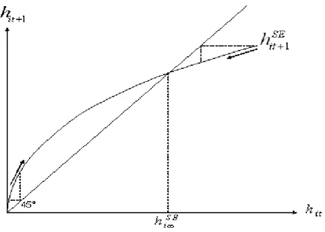
Figure 4 shows how the initial distribution of human capital contracts to a one-point distribution at steady state. The two arrows show how agents’ human capital evolves during the transition process from their initial position to the steady state level of human capital. Let us now consider equilibrium with an active labor market.
7.2
The equilibrium with multiple occupations
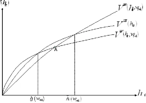
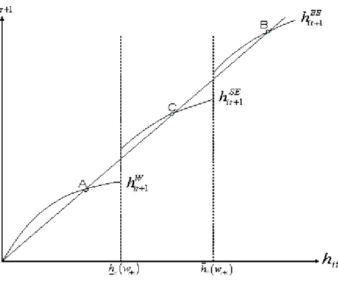
Two types of equilibrium with multiple occupations may occur in this economy. In the …rst one there are two occupations: the workers and the EE entrepreneurs. This equilibrium is the same that the one de…ned in the basic model. In the second type of equilibrium there exist three types of occupation: the workers, the SE entrepreneurs and the EE entrepreneurs. Figure 5 illustrates the two and three occupations equilibrium.
Figure 5: Two and Three Occupations Equilibrium
As seen in Figure 5, in a two-occupations equilibrium, the indirect utility function of EE entrepreneurs VEE(hit; wt+1) crosses the indirect utility function of workers VW(hit; wt+1) at the point A, which separates
the agents in the two categories. Point A corresponds to the occupational threshold ~hit(wt+1) de…ned in
the basic model. In a three occupations equilibrium, we have two thresholds: the …rst one, hit(wt+1) in
Figure 5, separates workers from SE entrepreneurs and the second one, hit(wt+1) in Figure 5, separates SE
entrepreneurs from EE entrepreneurs. From hminto h
it(wt+1) the indirect utility function of being a worker
is the highest one and agents with human capital level in this range choose to become workers. Between hit(wt+1) and hit(wt+1) the indirect utility function of being SE entrepreneur, VSE(hit), is the highest one
and the agents with human capital level in this range choose to become self-entrepreneurs. Finally, from hit(wt+1) to hmax the indirect utility function of being EE entrepreneurs is the highest one, therefore the
agents with human capital in this range choose to become employer-entrepreneurs.
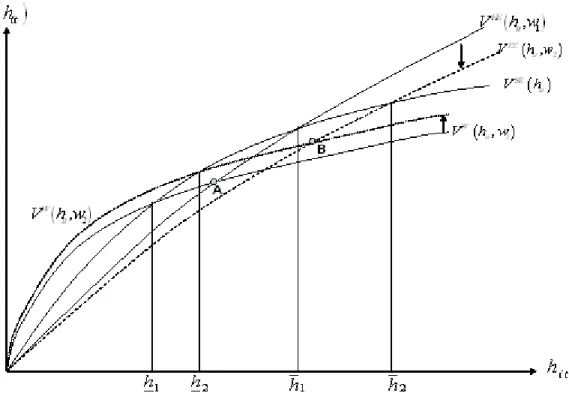
The only multiple occupations equilibrium which occurs is the three occupations equilibrium. As illus-trated in Figure 6 a two occupations equilibrium is always dominated by a three occupations equilibrium.
Figure 6: A Two Occupations Equilibrium is Always Dominated
In Figure 6 we exhibit the two and three occupations equilibrium at two wage levels, w1 and w2 with
w2> w1. When the wage equilibrium is w1the curve VSE(hit) is above the point A and the agents between
h1 and h1 are better o¤ being self-entrepreneurs. Therefore the two occupations equilibrium is dominated
by the three occupations equilibrium. As the equilibrium wage increases up to w2, VW(hit; wt+1) move up
while VEE(h
it; wt+1) move down . This implies that the two occupations thresholds move from h1 and h1
to, respectively, h2and h2 in Figure 6, and the two occupations equilibrium moves from point A to point B.
As seen in Figure 6, VSE(h
it) is still above the two occupations equilibrium (point B) when the equilibrium
wage increases. If the equilibrium wage increases enough for VW(h
it; wt+1) to rise above VSE(hit) for
any level of human capital, then all agents prefer to become workers and we fall into the one occupation equilibrium case. It is the same if the equilibrium wage decreases enough for all agents to prefer to become employer-entrepreneurs. Therefore the two occupations equilibrium never occurs in this context.
Proposition 7 A multiple occupations equilibrium is always a three occupations equilibrium.
Proof. It is easy to check that there is no equilibrium wage wt+1for which ht+1(wt+1) = ht+1(wt+1). This
condition is su¢ cient to guarantee that the two occupations equilibrium never occurs. In a three occupations equilibrium, the labor market equilibrium condition is:
Z hit(wt+1) hmin it hWit+1d (hit) = Z hmaxit h(wt+1) wt+1 1 1 hW Eit+1 1 hW Eit+1d (hit) (35)
where the …rst human capital threshold17h
it(wt+1) = Cw 1 ( + 1)
t+1 is given by the condition Vw(hit; wt+1) =
VSE(h
it), and the second human capital threshold hit(wt+1) = Bw 1 ( + 1)
t+1 is given by the condition
VSE(hit) = VEE(hit; wt+1).
Proposition 8 : At any date t, given the distribution of human capital, there exists a unique equilibrium with three occupations, characterized by the two occupation thresholds, hit and hit, and the equilibrium wage
wmin< w
t+1 wmax.
Proof. It follows the same principle of the proof of proposition 2.
This proposition states that, at equilibrium, there is a unique equilibrium wage which separates the agents across the three occupations. Therefore, there is endogenous formation of inequality since the human capital thresholds that separate the di¤erent categories of agents depend on the equilibrium wage.
The distribution of human capital is determinant for the types of equilibrium which arise and for the degree of inequality in the economy. The two dimensions of the distribution of human capital are important for the determination of the type of the equilibrium. The …rst dimension is the gap between hmin and
hmax. The greater the gap, the more likely it is that a three occupations equilibrium will occur. The second
dimension is the density of the distribution of human capital, which is de…ned by the dispersion of agents in the range hmin; hmax . The concentration of agents in the bottom, middle or top of the distribution
in‡uences the level of the equilibrium wage and therefore the type of occupation equilibrium which occurs. For instance, if there are many agents in the bottom of the distribution and there is a big gap between hmin and hmax, as is likely in poor countries, then the equilibrium wage will be low, implying many workers earning low revenues. In that case, a few entrepreneurs can hire all the labor supply for a low wage, magnifying inequality.
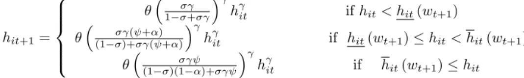
In a three occupations equilibrium, the dynamics of the economy are given by the evolution of the three human capital levels and of the equilibrium wage:
hit+1= 8 > > > < > > > : 1 + hit if hit< hit(wt+1) ( + ) (1 )+ ( + ) hit if hit(wt+1) hit< hit(wt+1) (1 )(1 )+ hit if hit(wt+1) hit (36)
Figure 7 illustrates this evolution of the human capital distribution and the short and long run three occu-pations equilibrium.
As seen in Figure 7, a speci…c curve of transition to a steady state is associated with each occupation with a speci…c level of investment in education. The employer-entrepreneurs invest more in education, therefore their human capital transition equation is the highest. Thus, at steady state there is a three-point distribution of human capital. Workers, self-entrepreneurs and employer-entrepreneurs converge, respectively, to point A, B, and C in Figure 7. Their respective long term levels of human capital are given by equations (14), (34) and (15).
De…ne
1as the long term fraction of workers in the economy and (1 1) as the long term fraction of
employer-entrepreneurs. One can de…ne also ^1 1
1 1 as the steady state ratio of workers to employer-1 7Fot the exact expression of the coe¢ cients C and B see the appendix.
Figure 7: Short and Long Run Three Occupations Equilibrium
entrepreneurs. Therefore, rewriting the steady state labor market equilibrium with three occupations yields the following relationship between the ratio of workers to EE entrepreneurs and the equilibrium wage:
^1(w1) = w1 1 1 + 1 (1 )(1 ) (1 ) (1 ) + 1 1 (37) 1 + 1 (1 + ) (1 ) (1 ) + 1
As ^1 is monotonic and decreasing with w1, the steady state equilibrium is unique. To summarize, Proposition 9 The steady state equilibrium with three occupations is characterized by a ratio of workers to EE entrepreneurs ^1, a unique equilibrium wage w1, and a three-point distribution of human capital. In that steady state, the level of human capital of an agent is either hW
i1 = 1 1 1 + 1 or hE i1 = 1 1 (1 )(1 )+ 1 , or hES1 = 11 ( + ) (1 )+ ( + ) 1 .
We have already shown that a multiple occupations equilibrium is a three occupations equilibrium. Thus, to demonstrate the existence of a steady state equilibrium with three occupations it su¢ ces to verify that at steady state some agents are better o¤ being workers while others are better o¤ being employer-entrepreneurs. That is, for some agents VW(hW1; w1(^1)) > VSE(hW1) while for others VEE(hE1; w1(^1)) > VSE(hE1; ). These two inequalities give a condition for the existence of equilibrium with three occupations. It is a range for the ratio of workers to entrepreneurs with employees, ^1 and a corresponding range for the equilibrium
wage. This existence condition is similar to condition (19). Therefore, we also have a continuum of steady states with three occupations.
Proposition 10 The equilibrium steady state of any initial distribution of human capital is a three occu-pations equilibrium if and only if ^1 < ^1(w1) < ^1+ and w1 < w1(^1) < w+
1: Thus, there exists a
continuum of steady state with three occupations.
The model is robust to an extension of the number of occupations. However, the extension creates the possibility of an equilibrium with equality of status and of human capital in the long run. Depending on the initial distribution of human capital, the model can exhibit long term inequality or long term equality. This result has some resemblance to Matsuyama’s [2000] model, but o¤ers a very di¤erent picture of the possible inequality con…gurations at steady state. The introduction of the storage technology in Matsuyama’s model creates the possibility of a steady state in which there is perfect equality, but it is an equalization of misery in which all the households remain poor. In our model, introducing the self-employment technology generates the possibility of a steady state in which there is perfect equality, but it is rather a middle class economy.
8
CONCLUDING REMARKS
Since Loury’s [1981] seminal paper, many contributions have emphasized the role of imperfect capital markets and wealth distribution on the formation and persistence of inequalities. Among many others, Galor and Zeira [1993], Banerjee and Newman [1993], Ljungqvist [1993], Durlauf [1996], Aghion and Bolton [1997], and Mookherjee and Ray [2003] have shown that both assumptions of imperfect capital markets and non-convex investment technology are key elements in generating the formation and persistence of inequalities.
In contrast to these analyses, this paper is built on the hypothesis that there is a di¤erence in the returns of low and high levels of human capital. This motivates agents’di¤erent investment in education and occupa-tional choice, given their inherited human capital level. Precisely, the model generates endogenous persistent inequality. There exists a unique human capital threshold which separates workers from entrepreneurs. In this model, agents less endowed in human capital have a comparative advantage in becoming workers, and thus invest less in education. Agents with a relatively higher endowment of human capital are better o¤ becoming entrepreneurs and invest more in education. These two classes of agents persist in the long run. However, there is room for upward or downward mobility during the transition process.
The model also exhibits a continuum of steady states, each of which is characterized by a two-point distribution and an equilibrium wage. This re‡ects the fact that economies with di¤erent initial human capital distribution converge to di¤erent steady states with di¤erent inequality levels. It is shown that there exists an optimal steady state among the continuum of steady states. The optimal steady state maximizes the sum of the utility of the agents in the economy. The government has the possibility of improving the competitive steady state equilibrium in order to bring it closer to the optimal one. Allowing for self-employment in the model generates the possibility of equality at equilibrium, in addition to the inequality equilibrium with three occupations.
Two critical hypotheses play a fundamental role in the results of this paper. The …rst key assumption is that the production function of the entrepreneurial project is an increasing returns to scale technology which depends on entrepreneurs’ speci…c level of human capital. This hypothesis leads to two pro…les of human capital returns in the economy, at least. For low levels of human capital, the return is linearly increasing with human capital, while for high levels of human capital the return is convexly increasing with human capital. This creates the break between entrepreneurs and workers in the earnings pro…les. The second key assumption is that the production of human capital is an increasing function of inherited human capital (parental human capital). The combination of the latter two hypotheses makes the occupational choice dependent on the inherited level of human capital.
The model has important implications for human capital returns in the economy. First, workers’human capital returns are lower than those of entrepreneurs. Secondly, the returns on workers’human capital are linear and increasing with their level of human capital, while the returns on entrepreneurs’ human capital are convex and increasing. Dominique Rouault [2001] showed that, in France, the revenue of entrepreneurs is greater on average than that of workers for each level of education. Moreover, he found that high levels of college attendance are better valued in entrepreneurship activity. Van der Sluis, Van Praag and Van Witteloostuijn [2004] found that the returns on education for entrepreneurs in the US are much higher than the returns for employees (respectively 14.2% and 10.7%). They also …nd that the returns on education turn out to follow a U shaped distribution for the two groups, but with signi…cant di¤erences between those two groups. There is a need to further investigate the di¤erence of returns on education for workers and entrepreneurs.
The model also emphasizes the role of inherited human capital in a broad sense on agents’trajectories. In that case, the policy debate remains open on whether it is preferable to focus on education to tackle ex-ante human capital (family e¤ects) inequality, or to focus on ex-post revenue redistribution. The model can be extended to take this alternative into account.
References
Aghion, P. and P. Bolton (1997). A theory of trickle-down growth and development. Review of Economic Studies 64:2, 151–172.
Banerjee, A. and A. Newman (1993). Occupational choice and the process of development. Journal of Political Economy 101, 274–298.
Becker, G. S. and N. Tomes (1979). An equilibrium theory of the distribution of income and intergenera-tional mobility. Journal of Political Economy 87 (6), 1153–1189.
Becker, G. S. and N. Tomes (1986). Human capital and the rise and fall of families. Journal of Labor Economics 4 (3), S1–S39.
Chatterjee, S. (1994). Transitional dynamics and the distribution of wealth in a neoclassical growth model. Journal of Public Economics 54, 97–119.
Dunn, T. and D. Holtz-Eakin (2000). Financial capital, human capital, and the transition to self-employment: Evidence from intergenerational links. Journal of Labor Economics 18 (2), 282–305. Durlauf, S. N. (1996). A theory of persistent income inequality. Journal of Economic Growth 1, 75–93. Galor, O. and O. Moav (2003). Das human kapital:a theory of the demise of the class structure. Brown
University.
Galor, O. and D. Tsiddon (1997). Technological progress, mobility and economic growth. American Eco-nomic Review 87 (3), 363–382.
Galor, O. and J. Zeira (1993). Income distribution and macroeconomics. Review of Economic Studies 60, 35–52.
Ghatak, M. and N.-H. Jiang (2001). A simple model of inequality, occupational choice, and development. University of Chicago Working Paper .
Glomm, G. and B. Ravikumar (1992). Public versus private investment in human capital: Endogenous growth and income inequality. Journal of Political Economy 100 (4), 818–834.
Ho¤, K. and J. Stiglitz (2001). Modern economic theory and development. In G. Meir and J. Stiglitz (Eds.), Frontiers of Development Economics. New York: World Bank and Oxford University Press. Ljungqvist, L. (1993). Economic underdevelopment: the case of missing market for human capital. Journal
of Development Economics 40 (2), 219–239.
Loury, G. C. (1981). Intergenerational transfers and the distribution of earnings. Econometrica 49 (4), 843–867.
Lucas, R. E. J. (1988). On the mechanics of economic development. Journal of Monetary Economics 22, 3–42.
Matsuyama, K. (2000). Endogenous inequality. Review of Economic Studies 67, 743–759.
Matsuyama, K. (2003). On the rise and fall of class societies. Working Paper Northwestern University. Mookherjee, D. and D. Ray (2002). Contractual structure and wealth accumulation. The American
Eco-nomic Review 92 (4), 818–849.
Mookherjee, D. and D. Ray (2003). Persistent inequality. Review of Economic Studies 70 (2), 369–394. Piketty, T. (1997). The dynamics of the wealth distribution and the interest rate with credit rationing.
Review of Economic Studies 64, 173–189.
Ray, D. (2004). On the dynamics of inequality. New York University, Working Paper .
Rouault, D. (2001). Les revenus des indépendants et dirigeants: la valorisation du bagage personnel. Economie et Statistique 8 (348), 35–59.
Van Der Sluis, J., C. V. Praag, and W. Witteloostuijn (2004). The returns to education: a comparative study between entrepreneurs and employees. Working Paper, University of Amsterdam.