HAL Id: inria-00591061
https://hal.inria.fr/inria-00591061
Submitted on 6 May 2011
HAL is a multi-disciplinary open access
archive for the deposit and dissemination of
sci-entific research documents, whether they are
pub-lished or not. The documents may come from
teaching and research institutions in France or
abroad, or from public or private research centers.
L’archive ouverte pluridisciplinaire HAL, est
destinée au dépôt et à la diffusion de documents
scientifiques de niveau recherche, publiés ou non,
émanant des établissements d’enseignement et de
recherche français ou étrangers, des laboratoires
publics ou privés.
Fine-grained parallelization of a Vlasov-Poisson
application on GPU
Guillaume Latu
To cite this version:
Guillaume Latu. Fine-grained parallelization of a Vlasov-Poisson application on GPU. Europar’10,
HPPC Workshop, Sep 2010, Ischia, Italy. �inria-00591061�
Fine-grained parallelization of a
Vlasov-Poisson application on GPU
Guillaume Latu1,2 1
CEA, IRFM, F-13108 Saint−Paul−lez−Durance, France.
2 Strasbourg 1 University & INRIA/Calvi project
Abstract. Understanding turbulent transport in magnetised plasmas is a subject of major importance to optimise experiments in tokamak fusion reactors. Also, simulations of fusion plasma consume a great amount of CPU time on today’s supercomputers. The Vlasov equation provides a useful framework to model such plasma. In this paper, we focus on the parallelization of a 2D semi-Lagrangian Vlasov solver on GPGPU. The originality of the approach lies in the needed overhaul of both numerical scheme and algorithms, in order to compute accurately and efficiently in the CUDA framework. First, we show how to deal with 32-bit floating point precision, and we look at accuracy issues. Second, we exhibit a very fine grain parallelization that fits well on a many-core architecture. A speed-up of almost 80 has been obtained by using a GPU instead of one CPU core. As far as we know, this work presents the first semi-Lagrangian Vlasov solver ported onto GPU.
1
INTRODUCTION
The present paper highlights the porting of a semi-Lagrangian Vlasov-Poisson code on a GPU device. The work, described herein, follows a previous study made on the loss code described in other papers [CLS06,CLS09,LCGS07]. A classical approach in the Semi-Lagrangian community involves the use of cubic splines to achieve the many interpolations needed by this scheme. The application we describe here, uses a local spline method designed specifically to perform decou-pled numerical interpolations, while preserving classical cubic spline accuracy. In previous papers, this scalable method was described, and was benchmarked in academic and industrial simulators. Only relatively small MPI inter-processor communication costs were induced and these codes scaled well over hundreds of cores (1D and 2D domain decompositions were investigated).
Particle-in-Cell (PIC) codes are often used in plasma physics studies and they use substantial computer time at some of the largest supercomputer centers in the world. Particle-in-Cell, yet less accurate, is a most commonly used numer-ical method than the semi-Lagrangian one. Several papers has been published on PIC codes that harness the computational power of BlueGene and GPGPU hardwares [SDG08,BAB+08] and provide good scalability. Looking for new
algo-rithms that are highly scalable in the field of Tokamak simulations is important to mimic plasma devices with more realism.
We will describe how to enrich the Semi-Lagrangian scheme in order to ob-tain scalable algorithms that fits well in the CUDA framework. In the sequel, the numerical scheme and the accuracy issues are briefly introduced and the parallelization of the main algorithm with CUDA is described. The speedup and accuracy of the simulations are reported and discussed.
2
MATHEMATICAL MODEL
In the present work, we consider a reduced model for two physical dimensions (in-stead of six in the general case), corresponding to x and vxsuch as (x, vx) ∈ R2.
The 1D variable x represents the configuration space and the 1D variable vx
stands for the velocity along x direction. Moreover, the self consistent magnetic field is neglected because vxis considered to be small in the physical
configura-tions we are looking at. The Vlasov-Poisson system then reads: ∂f
∂t + vx.∇xf + (E + vx× B) .∇vxf = 0, (1)
−ε0∇2φ = ρ(x, t) = q
Z
f (x, vx, t)d vx, E(x, t) = −∇φ. (2)
where f (x, vx, t) is the particle density function, ρ is the charge density, q is
the charge of a particle (only one species is considered) and ε0 is the vacuum
permittivity, B is the applied magnetic field.
Eq. (1) and (2) are solved successively at each time step. The density ρ is evaluated in integrating f over vx and Eq. (2) gives the self-consistent
electro-static field E(x, t) generated by particles. Our work focuses on the resolution of Eq. (1) using a backward semi-Lagrangian method [SRBG99]. The physical domain is defined as D2
p = {(x, vx) ∈ [xmin, xMax] × [vxmin, vxMax]}. For the sake
of simplicity, we will consider that the size of the grid mapped on this physical domain is a square indexed on D2
i = [0, 2j− 1]2(it is easy to break this
assump-tion to get a rectangle). Concerning the type of boundary condiassump-tions, a choice should be made depending on the test cases under investigation. At the time being, only periodic extension is implemented.
3
ALGORITHMIC ANALYSIS
3.1 Global numerical scheme
The Vlasov Equation (1) can be decomposed by splitting. It is possible to solve it, through the following elementary advection equations:
∂tf + vx∂xf = 0, (ˆx operator) ∂tf + ˙vx∂vxf = 0. (ˆvx operator)
Each advection consists in applying a shift operator. A splitting of Strang [CK76] is employed to keep a scheme of second order accuracy in time. We took the sequence (ˆx/2, ˆvx, ˆx/2), where the factor 1/2 means a shift over a reduced time
step ∆t/2. Algorithm 2 shows how the Vlasov solver of Eq. (1) is interleaved with the field solver of Eq. (2).
3.2 Local spline method
Each 1D advection (along x or vx) consists in two substeps (Algorithm 1). First,
the density function f is processed in order to derive the cubic spline coefficients. The specificity of the local spline method is that a set of spline coefficients covering one subdomain can be computed concurrently with other ones. Thus, it improves the standard approach that unfortunately needs a coupling between all coefficients along one direction. Second, spline coefficients are used to interpolate the function f at specific points. This substep is intrinsically parallel wether with the standard spline method or with the local spline method: one interpolation involves only a linear combination of four neighbouring spline coefficients.
In Algorithm 1, xo is called the origin of the characteristic. With the local
spline method, we gain concurrent computations during the spline coefficient derivation (line 2 of the algorithm). Our goal is to port Algorithm 1 onto GPU.
Algorithm 1: Advection in x dir., dt time step Input : f
Output: f forallvxdo 1
a(.) ← spline coeff. of sampled function f (., vx) 2 forallx do 3 x0← x − v x.dt 4
f (x, vx) ← interpolate f (x0, vx) with a(.) 5
Algorithm 2: One time step Input : ft
Output: ft+∆t
// Vlasov solver, part 1 1D Advection, operatorˆx 2 on f (., ., t) 1 // Field solver Integrate f (., ., t+∆t/2) over vx 2 to get density ρ(., t+∆t/2) 3
Compute Φt+∆t/2with Poisson solver 4
using ρ(., t+∆t/2)
5
// Vlasov solver, part 2
1D Advection, operator ˆvx(use Φt+∆t/2) 6
1D Advection, operatorˆx 2 7
3.3 Floating point precision
Usually, semi-Lagrangian codes make extensive use of double precision float-ing point operations. The double precision is required because pertubations of small amplitude often play a central role during plasma simulation. For the sake of simplicity, we focus here on the very classical linear Landau damping test case (with k = 0.5, α = 0.01) which highlights the accuracy problem one can ex-pect in Vlasov-Poisson simulation. The initial distribution function is given by f (x, vx, 0) =e
−vx 2 2
√2
π (1 + α cos(k x)) . Other test cases are available in our
imple-mentation, such as strong Landau damping, or two stream instability. They are picked to test the numerical algorithm and for benchmarking.
The problem arising with single precision computations is shown on Fig. 1. The reference loss code (CPU version) is used here. The L2norm of electric potential
is shown on the picture (electric energy) with logarithmic scale along the Y-axis. The double precision curve represents the reference simulation. The difference between the two curves indicates that single precision is insufficient; especially for long-time simulation. With an accurate look at the figure, one can notice that the double precision simulation is accurate until reaching a plateau value near 10−20. To go beyond this limit, a more accurate interpolation is needed.
3.4 Improvement of numerical precision
For the time being, one has to consider mostly single precision (SP) computations to get maximum performance out of a GPU. The double precision (DP) is much slower than single precision (SP) on today’s devices. In addition, the use of double precision may increase pressure on memory bandwidth.
-25 -20 -15 -10 -5 0 20 40 60 80 100 120 140 single precision double precision
Fig. 1. Electric energy for Landau test case 10242, single versus double precision
(depending on time measured as a num-ber of plasma period ωc−1)
-25 -20 -15 -10 -5 0 20 40 60 80 100 120 140 single precision double precision deltaf single precision deltaf double precision
Fig. 2. Electric energy for Landau test case 10242, using δf
represen-tation or standard representation.
The previous paragraph shows that SP leads to unacceptable numerical re-sults. It turns out that our numerical scheme could be modified to reduce nu-merical errors even with only SP operations during the advection steps. To do so, a new function δf (x, vx, t) = f (x, vx, t) − fref(x, vx) is introduced. Working
on the δf function could improve accuracy if the values that we are working on are sufficiently close to zero. Then, the reference function fref should be chosen
such that the δf function remains relatively small (in L∞ norm). convenient to assume that fref is a constant along the x dimension. For the Landau test case,
we choose fref(vx) = √12
πe−
vx2
2 . As the function f
ref is constant along x, the
x-advection applied on frefleaves frefunchanged. Then, it is equivalent to apply
ˆ
x operator either on function δf or on function f . Working on δf is very worth-wile (ˆx operator): for the same number of floating point operations, we increase accuracy in working on small differences instead of large values. Concerning the
ˆ
vxoperator however, both frefand f are modified. For each advected grid point
(x, vx) of the f⋆ function, we have (vxo is the foot of the characteristic):
f⋆(x, vx) = f (x, vxo) = δf (x, vxo) + fref(vxo), δf⋆(x, vx) = f⋆(x, vx) − fref(vx),
δf⋆(x, vx) = δf (x, vxo) − (fref(vx) − fref(vxo)).
Working on δf instead of f changes the operator ˆvx. We now have to interpolate
both δf (x, vo
x) and (fref(vx)−fref(vox)). In doing so, we increase the number of
computations; because in the original scheme we had only one interpolation per grid point (x, vx), whereas we have two in the new scheme. In spite of this cost
increase, we enhance the numerical accuracy using δf representation (see Fig. 2). A sketch of the δf scheme is shown in Algorithm 3.
4
CUDA ALGORITHMS
4.1 CUDA Framework
Designed for NVIDIA GPUs (Graphics Processing Units), CUDA is a C-based general-purpose parallel computing programming model. Using CUDA, GPUs can be regarded as coprocessors to the central processing unit (CPU). They communicate with the CPU through fast PCI-Express ports. An overview of the CUDA language and architecture could be found in [NVI09]. Over the past few years, some success in porting scientific codes to GPU have been reported in the literature. Our reference implementation of loss, used for comparisons, uses Fortran 90 and MPI library. Both sequential and parallel versions of loss have been optimized over several years. The CUDA version of loss presented here mixes Fortran 90 code and external C calls (to launch CUDA kernels).
Algorithm 3: One time step, δf scheme Input : δft Output: δft+∆t 1D advection on δf , operator ˆx 2 1 Integrate δf (., ., t+∆t/2) + fref(.) 2 to get ρ(., t+∆t/2) 3 Compute Φt+∆t/2, 4
with Poisson solver on ρ(., t+∆t/2)
5
1D advection on δf , operator ˆvx 6
→ stored into δf
7
Interpolate fref(vx) − fref(vox) 8
→ results added into δf
9
1D advection on δf , operator ˆx 2 10
Algorithm 4: Skeleton of an advection kernel Input : ftin global memory of GPU
Output: ft+dtin global memory of GPU
// A) Load from global mem. to shared mem. Each thread loads 4 floats from global mem.
1
Floats loaded are stored in shared memory
2
Boundary conditions are set (extra floats are read)
3
Synchro.: 1 thread block owns n vectors of 32 floats
4
// B) LU Solver
1 thread over 8 solves a LU system (7 are idle)
5
Synchro.: 1 block has n vectors of spline coeff.
6
// C) Interpolations
Each thread computes 4 interpolations
7
// D) Writing to GPU global memory Each thread writes 4 floats to global mem.
8
4.2 Data placement
We perform the computation on data δf of size (2j)2. Typical domain size varies
from 128 × 128 (64 KB) up to 1024 × 1024 (4 MB). The whole domain fits easily in global memory of current GPUs. In order to reduce unnecessary overheads, we decided to avoid transfering 2D data δf between the CPU and the GPU as far as we can. So we kept data function δf onto GPU global memory. CUDA computation kernels update it in-place. For diagnostics purposes only, the δf function is transfered to the RAM of the CPU at a given frequency.
4.3 Spline coefficients computation
Spline coefficients (of 1D discretized functions) are computed on patches of 32 values of δf . As explained elsewhere [CLS06], a smaller patch would introduce significant overhead because of the cost of first derivative computations on the patch borders. A bigger patch would increase the computational grain which is a bad thing for GPU computing that favors scheduling large number of threads. The 2D domain is decomposed into small 1D vectors (named “patches”) of 32 δf values. To derive the spline coefficients, tiny LU systems are solved. The
assembly of right hand side vector used in this solving step can be summarized as follows: keep the 32 initial values, add 1 more value of δf at the end of the patch, and then add two derivatives of δf located at the borders of the patch. Once the right hand side vector is available (35 values), two precomputed matrices L and U are inverted to derive spline coefficients (using classical forward/backward substitution). We decided not to parallelize this small LU solver: a single CUDA thread is in charge of computing spline coefficients on one patch That point could be improved in the future in order to use several threads instead of one. 4.4 Parallel interpolations
On one patch, 32 interpolations need to be done (except at domain boundaries). These interpolations are decoupled. To maximize parallelism, one can even try to dedicate one thread per interpolation. Nevertheless, as auxiliary computa-tions could be factorized (for example the shift vx.dt at line 4 of Algo. 1), it is
relevant to do several interpolations per thread to reduce global computation cost. The number of such interpolations per thread is a parameter that impacts performance. This blocking factor is denoted K.
4.5 Data load
The computational intensity of the advection step is not that high. During the LU phase (spline coefficients computation), each input data is read and written twice and generates two multiplications and two additions in average. During the interpolation step, there are four reads and one write per input data and also four multiplications and four additions. The low computational intensity implies that we could expect shortening the execution time in reducing loads and writes from/to GPU global memory. So, there is a benefit to group the spline computation and the interpolations in a single kernel. Several benchmarks have confirmed that with two distinct kernels (one for building splines and one for interpolations) instead of one, the price of load/store in the GPU memory increases. Thus, we now describe the solution with only one kernel.
4.6 Domain decomposition and fine grain algorithm
We have designed three main kernels. Let us give short descriptions: KernVA operator ˆvx on δf (x, vx), KernVB adding fref(vx) − fref(vxo) to δf (x, vx), KernX
operator ˆx on δf (x, vx). The main steps of KernVA or KernX are given in
Algo-rithm 4. The computations of 8 n threads acting on 32 n real number values are described (it means K = 4 hardcoded here).
First A) substep reads floats from GPU global memory and puts them into fast GPU shared memory. When entering the B) substep, all input data have been copied into shared memory. Concurrently in the block of threads, small LU sys-tem are solved (but 87% of the threads stays idle). Spline coefficients are then stored in shared memory. In substep C), each thread computes K = 4 interpola-tions using spline coefficients. This last task is the most computation intensive part of the simulator. Finally, results are written into global memory.
5
PERFORMANCE
5.1 Machines
In order to develop the code and perform small benchmarks, a cheap personal computer has been used. The CPU is a dual-core E2200 Intel (2.2Ghz), 2 GB of RAM, 4 GB/s peak bandwidth, 4 GFLOPS peak, 1 MB L2 cache. The GPU is a GTX260 Nvidia card: 1.24 Ghz clock speed, 0.9 GB global memory, 95 GB/s peak bandwidth, 750 GFLOPS peak, 216 cores. Another computer (at CINES, FRANCE) has been used for benchmarking. The CPU is a bi quad-core E5472 Harpertown Intel (3 Ghz), 1 GB RAM, 5 GB/s peak bandwidth, 12 GFLOPS peak, L2 cache 2×6 MB. The machine is connected to a Tesla S1070, 1.44Ghz, 4 GB global memory, 100 GB/s peak bandwidth, 1000 GFLOPS peak, 240 cores.
5.2 Small test case
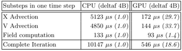
Substeps in one time step CPU (deltaf 4B) GPU (deltaf 4B)
X Advection 5123 µs (1.0 ) 172 µs (29.7 )
V Advection 4850 µs (1.0 ) 144 µs (33.7 )
Field computation 133 µs (1.0 ) 93 µs (1.4 )
Complete Iteration 10147 µs (1.0 ) 546 µs (18.6 )
Table 1. Computation times inside a time step and speedup (in
parentheses) averaged over 5000 calls - 2562 Landau test case,
E2200/GTX260
Let us first have a look on performance of the δf scheme. We consider the small testbed (E2200-GTX260), and a reduced test case (2562domain). The simulation
ran on a single CPU core, then on the 216 cores of the GTX260. Timing results and speedups (reference is the CPU single core) are given in Table 1. The speedup is near 30 for the two significant computation steps, but is smaller for the field computation. The field computation part includes two substeps: first the integral computations over the 2D data distribution function, second a 1D poisson solver. The timings for the integrals are bounded up by the loading time of 2D data from global memory of the GPU (only one addition to do per loaded float). The second substep that solves Poisson equation is a small sequential 1D problem. Furthermore, we loose time in lauching kernels on the GPU (25 µs per kernel launch included in timings shown).
Substeps in one time step
CPU (deltaf 4B) GPU (deltaf 4B) X Advections 79600 µs (1.0 ) 890 µs (90 ) V Advections 89000 µs (1.0 ) 1000 µs (89 ) Field computation 1900 µs (1.0 ) 180 µs (11 ) Complete Iteration 171700 µs (1.0 ) 2250 µs (76 ) Table 2.Computation time and speedups (in parenthe-ses) averaged over 5000 calls - 10242Landau test case -E2200/GTX260
Substeps in one time step
CPU (deltaf 4B) GPU (deltaf 4B) X Advections 67000 µs (1.0 ) 780 µs (86 ) V Advections 42000 µs (1.0 ) 960 µs (43 ) Field computation 1500 µs (1.0 ) 200 µs ( 7 ) Complete Iteration 110000 µs (1.0 ) 2200 µs (50 ) Table 3.Computation time and speedups (in parenthe-ses) averaged over 5000 calls - 10242Landau test case -Xeon/Tesla1070
5.3 Large test case
In Tables 2-3, we look at a larger test case with data size equal to 10242.
Com-pared to a single CPU core, the advection kernels have speedups from 75 to 90 for a GPU card (using260 000 threads). Here, the field computation represents a small computation compared to the advections and the low speedup for the field solver is not a real penalty. A complete iteration reaches a speedup of 76.
CONCLUSION
It turns out that δf method is a valid approach to perform a Semi-Lagrangian Vlasov-Poisson simulation using only 32-bit floating-point precision instead of classical 64-bit precision. So, we have described the implementation on GPU of the advection operator used in Semi-Lagrangian simulation with δf scheme and single precision. A very fine grain parallelization of the advection step is presented that scales well on thousands of threads. We have discussed the kernel structure and the trade-offs made to accommodate the GPU hardware.
The application is bounded up by memory bandwidth because computational intensity is small. It is well known that algorithms of high computational inten-sity are able to be efficiently implemented on GPU. We have demonstrated that an algorithm of low computational intensity can also benefit from GPU hard-ware. Our GPU solution reaches a significant speedup of overall 76 compared to a single core CPU execution. In the near future, we expect to have a solution for 4D semi-Lagrangian codes (2D space, 2D velocity) that runs on a GPU cluster.
References
[BAB+08] K. J. Bowers, B. J. Albright, B. Bergen, L. Yin, K. J. Barker, and D. J.
Kerbyson. 0.374 pflop/s trillion-particle kinetic modeling of laser plasma interaction on roadrunner. In Proc. of Supercomputing. IEEE Press, 2008. [CK76] C.Z. Cheng and Georg Knorr. The integration of the Vlasov equation in
configuration space. J. Comput Phys., 22:330, 1976.
[CLS06] N. Crouseilles, G. Latu, and E. Sonnendr¨ucker. Hermite spline interpolation on patches for a parallel solving of the Vlasov-Poisson equation. Technical Report 5926, INRIA, 2006. http://hal.inria.fr/inria-00078455/en/.
[CLS09] N. Crouseilles, G. Latu, and E. Sonnendr¨ucker. A parallel Vlasov solver based on local cubic spline interpolation on patches. J. Comput. Phys., 228(5):1429–1446, 2009.
[LCGS07] G. Latu, N. Crouseilles, V. Grandgirard, and E. Sonnendr¨ucker. Gyrokinetic semi-lagrangian parallel simulation using a hybrid OpenMP/MPI program-ming. In PVM/MPI, pages 356–364, 2007.
[NVI09] NVIDIA. CUDA Programming Guide, 2.3, 2009.
[SDG08] George Stantchev, William Dorland, and Nail Gumerov. Fast parallel particle-to-grid interpolation for plasma PIC simulations on the GPU. J. Parallel Distrib. Comput., 68(10):1339–1349, 2008.
[SRBG99] E. Sonnendr¨ucker, J. Roche, P. Bertrand, and A. Ghizzo. The semi-lagrangian method for the numerical resolution of the Vlasov equations. J. Comput. Phys., 149:201–220, 1999.