WORKING
PAPERS
SES
N. 464
XI.2015
Optimal Social Insurance
and Health Inequality
Volker Grossmann
and
Optimal Social Insurance and Health Inequality
∗
Volker Grossmann
†and Holger Strulik
‡November 12, 2015
Abstract
This paper integrates into public economics a biologically founded, stochastic pro-cess of individual ageing. The novel approach enables us to investigate the interaction between health and retirement policy in order to quantitatively characterize the op-timal joint design of the social insurance system today and in response to future medical progress, and its implications for health inequality. Calibrating our model to Germany, we find that currently the public health and pension system is approxi-mately optimal. Future progress in medical technology calls for a potentially drastic increase in health spending that typically shall be accompanied with a lower pension savings rate and a higher retirement age. Medical progress and higher health spending is predicted to lead to more health inequality.
Key words: Ageing; Health Expenditure; Health Inequality; Social Security
System; Retirement Age.
JEL classification: H50; I10; C60.
∗We are grateful to seminar participants at the CESifo Area Conference in Public Sector Economics in
Munich, particularly our discussant Ngo van Long, the Annual Congress of the International Institute of Public Finance (IIPF) in Lugano, particularly our discussant Fabrizio Mazzonna, and the Annual Congress of the European Economic Association (EEA) in Toulouse, particularly Gr´egory Ponthi`ere, the University of Fribourg and the Free University of Berlin, particularly Giacomo Corneo, for valuable comments and suggestions. Financial support of the Swiss National Fund (SNF) and Deutsche Forschungsgemeinschaft (DFG) which co-finance the project “Optimal Health and Retirement Policy under Biologically Founded Human Ageing” (with SNF as ‘lead agency’) is gratefully acknowledged.
†University of Fribourg, Switzerland; CESifo, Munich; Institute for the Study of Labor (IZA), Bonn;
Centre for Research and Analysis of Migration (CReAM), University College London. Postal address: University of Fribourg, Department of Economics, Bd. de P´erolles 90, CH-1700 Fribourg. E-mail: [email protected].
‡University of Goettingen. Postal address: University of Goettingen, Department of Economics, Platz
1
Introduction
Life expectancy of adults increased by around 15 years over the 20th century and many researchers in demography and the natural sciences consider it likely to increase further (e.g. Gavrilov and Gavrilova, 1992; Oeppen and Vaupel, 2002). The development was to a large extent driven by fast advances in medical and pharmaceutical research that led to substantial increases in the effectiveness of health spending on the ageing process.1 Through this channel, health spending contributes to the widely discussed problem of social security systems, namely that pension payments are likely to decline for a given pension savings rate unless the statutory retirement age is changed. This implies that health and pension policy shall be examined and designed jointly.
Higher effectiveness of medical technology may make higher contribution rates to public health insurance more desirable in order to better reap the benefits in terms of improved health and higher life expectancy. Its adverse effect on pension payments could be offset by raising contributions to the pension system as well. There is, however, a trade-off between the two tiers of the social insurance system, as higher contributions to pension insurance and health insurance both reduce net income in the working period, for a given labor supply and because of a reduction in labor supply. Alternatively, it could be desirable to increase the retirement age along with an increase in health spending. In view of the complex linkages between the pension system and the health care system created by the endogeneity of human health and longevity, the jointly optimal design of our social insurance systems appears to be both important and a priori non-obvious.
This paper investigates the interactions between public health and pension policy in order to quantitatively characterize the optimal joint design of the social insurance system today and in response to future medical progress. In line with a long tradition in public economics to justify social systems, we focus on welfare maximization behind the veil of ignorance. It is based on the idea that an ex ante identical population would agree on a 1Medical and pharmaceutical innovations became important drivers of life expectancy from the 1950s
onwards. Before that, life expectancy rose predominantly because of decreases in child mortality rather than because of increases in life expectancy of adults (e.g. Milligan and Wise, 2011). In the US, the fraction of the population which is at least 65 years old is projected to be 18.8 percent in 2025, whereas it was 8.1 percent in 1950 (Poterba, 2014).
social insurance system which reduces the probability of illness and insures against social hardships and long life. An interesting, related question is whether implementing an ex
ante optimal health care system will reduce health inequality within a society compared to
the status quo. In fact, reducing health inequality is a major goal of large organizations like the World Health Organization (WHO) and the European Union (EU).2 It is, however, non-obvious whether it is line or in conflict with the goal to maximize ex ante welfare.
Our key innovation which enables us to examine these issues is to integrate into public economics a biologically founded process of individual ageing. Ageing is understood as the stochastic and individual-specific deterioration of the functioning of body and mind − represented by an accumulation of health deficits − that eventually culminates in death (Arking, 2006; Masoro, 2006). Our approach is based on empirical evidence from gerontol-ogy3 which suggests that (i) at any given age, the number of health deficits is approximately Poisson-distributed in the population, (ii) the average number of individual health deficits grows with age, and (iii) the probability of death strongly depends on the number of health deficits an individual has accumulated over time (Mitnitski and Rockwood, 2002a, 2002b, 2005).
A salient feature of our analysis is that, insofar as health expenditures targeted to the working-aged affect the distribution of health deficits in this group, they also affect the distribution of health deficits among retirees. Consequently, improving health of the working-aged raises life expectancy for individuals at retirement age and ceteris paribus reduces pension payments. It also raises the productivity of workers and their contributions to the social insurance system, with positive effects on pension payments. Accordingly, we distinguish health care expenses for the working-aged from health expenditure targeted to typical illnesses of the elderly. Examples of the former would be expenses for mass examinations of the health status of pupils at schools, costs for educational health campaigns 2See www.who.int and www.health-inequalities.eu/. According to the WHO, health inequality is defined
as “differences in health status or in the distribution of health determinants between different population groups”.
3Modern gerontology tries to explain human ageing by employing basic insights and mechanisms from
reliability theory, which describes the human organism as a complex, redundant system (Gavrilov and Gavrilova, 1991). The notion of ageing as accelerated loss of organ reserve is in line with the mainstream view in the medical science. For example, initially, as a young adult, the functional capacity of human organs is estimated to be tenfold higher than needed for survival (Fries, 1980).
(about nutrition, usage of soft drugs, prevention of HIV infections etc.), and expenses for treating health problems and curing illnesses which typically also hit younger adults, like type 1 diabetes, virus infections, bacterial infections, orthopedic issues after accidents, psychiatric problems. Examples of expenses affecting the distribution of health deficits of retirees conditional on the distribution of health deficits of the working-aged are those treating cardiovascular diseases, type 2 diabetes, cancer, stroke, lung disease, and arthrosis. We measure health inequality of workers and retirees separately by the Gini coefficient of these distributions.
The main assumption that keeps the analysis tractable and the numerical results well interpretable is that workers fully rely on the public (PAYG) pension system to finance old-age consumption. A prime candidate for examining the optimal design of a social in-surance system in such a context is Germany, where private inin-surance for health purposes and private old age savings quantitatively play a minor role.4 Retired households received about 80 percent of income from social security in the 1990s (B¨orsch-Supan and Schnabel, 1998). Empirical evidence also suggests that assuming agents who do not adjust private savings when public pension policy changes well describes the behavior of the vast majority of individuals (Chetty, 2015). For instance, in the year 2002, in Germany a subsidized private annuity market scheme started operating that was similar to the subsidized IRA accounts in the US. The public subsidies in this so-called “Riester -scheme” are especially high as a percentage of contributions for low income households with children. They were accompanied by heavy marketing campaigns of the federal government and insurance com-panies. Moreover, there was a wide discussion of demographic changes and the implications on the public pension system in the media. Indeed, about 11 million contracts have been signed until the end of March 2008. Nevertheless, the impact of the subsidies on savings in private annuity market was negligible (Corneo, Keese and Schr¨oder, 2009; B¨orsch-Supan et al., 2015). This suggests that the saving volumes defined in the contracts were low and/or they replaced other forms of private annuity savings (that had already low volumes for the 4That said, the scope of our study certainly extends to other advanced countries. For instance, in the
US, social security is the most important source of support of retirees for the bottom half of the income distribution (Poterba, 2014). Financial assets outside retirement accounts play a minor role for the vast majority of households.
bulk of households to begin with).
The analytical part first establishes the links between health spending and pension payments that works via the endogeneity of life expectancy. We further show that the optimal allocation of health spending is typically tilted to the working-aged compared to the one that would maximize life expectancy. The main reason is that maximizing life expectancy may conflict with the goal to receive high contributions to the pension system of a productive workforce. The numerical part suggests that the status quo health system in Germany is approximately optimal. The possibility to prolong life via future medical progress shall be exploited by possibly drastically increasing the health contribution rate. To limit the increase in the total tax burden individuals typically prefer to lower the pensions savings rate at the same time, accompanied by a higher retirement age. Also interestingly, more health spending as an optimal response to a more powerful medical technology, as a rule, leads to more health inequality. The reason is that there are disproportionately large gains in life expectancy for those who develop only a small number of health deficits to begin with. Our analysis also shows that, in most cases, individuals prefer to increase the retirement age by a smaller factor than life expectancy expands.
After reviewing the related literature in section 2, we develop in section 3 a theoreti-cal model based on evidence from gerontology. It highlights the fundamental interactions between public pensions and health spending targeted to working-aged individuals and retirees. In section 4, we analytically characterize the optimal allocation of health care expenses for working-aged individuals and retirees by abstracting from the stochastic na-ture of the ageing process for simplicity. Section 5 calibrates our stochastic framework to Germany, which has a public pay-as-you-go (PAYG) system for both health care and pen-sions. Section 6 conducts numerical analysis to derive the currently optimal joint design of health and pension policy and studies the implications of the suggested policy reform on health, life expectancy, and health inequality. Section 7 examines how the optimal policy design should adjust when medical technology further improves and what it implies. The last section concludes.
2
Related Literature
In order to measure human functionality the medical science has proposed several indices of human capability or disability. The theory and calibration approach in the present paper is based on the so-called frailty index, which is particularly related to reliability theory (Gavrilov and Gavrilova, 1991).5 The frailty index is computed for a large sample of individuals and gives the fraction of the bodily impairments which are actually present out of a long list of potential impairments, ranging from mild deficits (reduced vision, incontinence) to near lethal ones (e.g. stroke). The evidence suggests that the frailty index of an individual correlates exponentially with age, that at any given age the number of deficits in a given population is approximately Poisson-distributed, and that the probability of death strongly depends on the number of health deficits that one has accumulated over time (e.g. Mitnitski and Rockwood, 2002a, 2002b, 2005). Associating health status with a simple count measure of health deficits is thus both appealingly simple and empirically successful. According to Rockwood and Mitnitski (2007) and Searle et al. (2008), the exact choice of the set of potential deficits is not crucial, provided that the set is sufficiently large. Another important insight from gerontology for the present paper is that individual deficit accumulation is path-dependent. Transitions in health status can be very accurately described by a Markov-chain augmented Poisson law according to which the probability to get another health deficit next period depends positively on the number of already accumulated health deficits (Mitnitski et al., 2006, 2007a, 2007b). This fact makes the simultaneous investigation of health and pension policy interesting and challenging.
Notwithstanding the advances in the natural sciences to understand life cycle health, the common conceptualization of health in economics is still based on the Grossman (1972) model.6 The basic idea of the Grossman model is that individuals accumulate health through investment in health capital, similar to the accumulation of human capital through investment in education. Without further amendments this means that desired health 5Strulik and Vollmer (2013) used the reliability approach of Gavrilov and Gavrilova (1991) to empirically
investigate its implications for long-run trends of human ageing and longevity.
6The basic Grossman framework has been extended in various directions (e.g. Ehrlich and Chuma, 1990;
expenditure drops at the point of retirement and that health depreciation is greater when the stock of health is large, that is when individuals are relatively young and healthy. Preserving health would thus require health expenditure to be high at working age and low at old age (for a critique, see Case and Deaton, 2005). In order to counteract this problem, the literature has assumed that the health depreciation rate is increasing with age. In contrast, modern gerontology suggests that individuals, as they age, do not accumulate health capital but health deficits.
Dalgaard and Strulik (2014) integrated into life cycle economics the notion of health deficit accumulation to understand the association between income and longevity. The model has also been applied to examine the education gradient in health and life expectancy (Strulik, 2013) and the long-run evolution of retirement behavior (Dalgaard and Strulik, 2012). So far, however, the theory was confined to life cycle decisions of a single agent. In the present paper we integrate physiological ageing into a novel equilibrium framework with two tiers of the social insurance system and endogenous longevity. We will first investigate the links between public health and pension policy for government budgets and their welfare effects. We then draw from these insights in order to characterize the optimal (i.e. welfare-maximizing) policy design.
There exists a relatively large literature discussing the impact of social security on labor supply and retirement and on the optimality or sustainability of public pension systems (e.g. Auerbach and Kotlikoff, 1987; Imrohoroglu, Imrohoroglu and Joines, 1995; B¨orsch-Supan, 2000; Jaag, Keuschnigg and Keuschnigg, 2010, 2011; see Liebman and Feldstein, 2002, for a survey). Particularly related to our paper is the study by Conesa and Krueger (1999) who like us study welfare effects of social security reform for an economy in which heterogenous individuals face a priori uncertainty about their ability (productivity). The interaction of pension finance and health care, however, is not investigated. Sinn (1995) showed that income redistribution is desirable by increasing risk-taking of expected utility maximizing individuals behind the veil of ignorance, i.e. before idiosyncratic ability is revealed. Conesa, Kitao and Krueger (2009) have used this concept in a macro model with idiosyncratic ability of workers and a social security system. The focus of their study, however, was not on optimal social security provision but on optimal income taxation.
While most of the conventional public pension literature ignores issues of health and longevity, there exists a smaller literature investigating the impact of health on labor supply and retirement when health is exogenous (Philipson and Becker, 1998; French, 2005; Heijdra and Romp, 2009; French and Jones, 2011; Imrohoroglu and Kital, 2012; Bloom, Canning and Moore, 2014) and when it is endogenously determined via the Grossman model of health capital accumulation (Wolfe, 1985; Galama et al., 2013). In Wolfe (1985), however, retirement is not determined by welfare maximization, and in Galama et al. (2013) longevity is not affected by health investment. Philipson and Becker (1998) investigate a life cycle model with given retirement age, longevity enhancing health expenditure, and (public) annuities. They argue that retired individuals demand too much health care because they do not take into account the effect of their longevity increasing behavior on the annuity level. They thus decide to live inefficiently long rather than to live well. Heijdra and Romp (2009) analyze the impact from pension reform in a general equilibrium setting, in the presence of a realistic – but exogenously given – mortality process. Bloom, Canning and Moore (2014) develop a life cycle model and use it to gauge the impact of changes in income and life expectancy on age of retirement. Calibration to the US suggests that the optimal retirement age decreases because of an income effect when wages grow despite increases in longevity. Health and longevity, however, are exogenously given.
Pestieau, Ponthi`ere and Sato (2008) argue that private health spending should be taxed when the replacement rate is sufficiently large. Leroux, Pestieau and Ponthi`ere (2011a,b) extend the model towards heterogenous agents who differ in their (genetically determined) probability of survival to retirement age. They show that optimal redistribution goes from high-productivity to low-productivity agents and from short-lived to long-lived individuals. While the available studies point to some interesting interaction of health and public policy they abstract from important other channels. Most importantly the available litera-ture focussed on the probability to reach an exogenously given retirement age and abstract from the effect of health on longevity, i.e. the years spent in retirement. The available liter-ature also did not take into account that idiosyncratic health endowments and health care during the working age of the population affects productivity and income and therewith the
health in old age, emphasized in the gerontological literature, remained unexplored. In this paper, we aim to overcome these shortcomings. We also attempt to fill an important gap in the existing literature by addressing the questions how health spending should be allocated over the life-cycle in interaction with the pension system and how health expenditure affects health inequality.
3
The Model
Consider the following continuous-time model. At each date t, a new cohort of ex ante identical individuals is born. The cohort size is time-invariant and normalized to unity. This assumption reflects our focus on the effects of ageing on the social insurance system caused by higher life expectancy rather than by (presumably temporary) changes in the birth rate. Ageing is stochastic in the sense that the deterioration process of health, and thus life-time, is stochastic. Life consists of a working period and a retirement period.
3.1
The Social Insurance System
The statutory retirement age (i.e. the length of the working period) is denoted by ¯R
and the same for all individuals, for simplicity. The government provides a health care system and a pension system to maximize ex ante welfare behind the veil of ignorance. Like in Germany, health expenditure and pension payments are financed by proportional social insurance contributions levied on labor income. There are separate budgets with contribution rates τh ∈ (0, 1) and τs ∈ (0, 1), respectively. Both systems are pay-as-you-go
(PAYG), i.e. the revenues are paid out contemporaneously and the budgets are balanced. We distinguish between health spending targeted to the working-aged population (e.g. for prevention programmes and curative care for illnesses that typically also hit younger adults, like virus infections and psychiatric problems) and health spending targeted to retirees (e.g. for treating illnesses typically related to old age, like cardiovascular diseases, cancer and arthrosis). The pension system is such that relative contributions between individuals of the same cohort to the system during the working period correspond to relative payments during
retirement in each point of time. Pension payments are time-invariant for an individual during the retirement period. There are no frictions in the system and pension income is not used to finance the social insurance system.
The government levies an additional, co-linear tax on labor income, τwI− T , where I is
labor income, τw is the marginal tax rate andT is referred to as “transfer” (think about an
earned income tax credit). As will become apparent, individuals with lower health status will supply less labor. Assuming a balanced budget, labor income taxation is therefore redistributive.
We abstract from private forms of health expenditure and pension insurance. Specifi-cally, a private annuity market is missing and individuals cannot save privately for the re-tirement period. This captures, albeit in a pronounced way, the little importance of private savings for retirement wealth for the vast majority of households in Germany (B¨orsch-Supan and Schnabel, 1998) for which we calibrate our model. The public pension system (‘social security’) is an important source of retirees’ income in the US as well (Poterba, 2014). Al-lowing for private pension savings to complement social security would enhance analytical complexity to the point of intractability in the case where life-time is uncertain. Assuming non-optimizing households with respect to old-age consumption is consistent with evidence from behavioral economics showing that most individuals stick to default pension plans offered by their employers (e.g. Chetty, 2015).7 Such evidence widely opens the scope for public policy, as discussed by Beshears et al. (2009), who survey the literature. Inter alia they point to evidence by Cronqvist and Thaler (2004) who show that the rate of return of the default portfolio in the Swedish social security system was higher than the perfor-mance of individuals who opted out of the default and selected the portfolio of assets by themselves.
7In an interesting recent paper, Caliendo and Findley (2013) derive the optimal social security
provi-sion in the US by analyzing a calibrated model in which individuals save an exogenous fraction of their disposable income. Under such non-optimizing behavior, the current size of the US social security program is supported.
3.2
Production
At each date, there is a single homogenous consumption good which is produced according to a neoclassical, constant-returns-to-scale production technology. Output Y is given by
Y = F (K, AL) ≡ ALf(k), k ≡ K
AL, (1)
where K and L are the inputs of physical capital and labor, the latter being measured in efficiency units. A is an exogenous measure of productivity. f (·) is strictly increasing, strictly concave, and fulfills the Inada conditions.
Output is sold in a perfectly competitive environment. The output price is normalized to unity. The rate of return to capital, r, is internationally given (i.e. we consider a small open economy assuming capital income is not taxed) and time-invariant. Thus, profit maximization of the representative firm implies that k is given by r = f′(k), i.e.
k = (f′)−1(r) ≡ ¯k(r). Consequently, the wage rate per efficiency unit of human capital reads as w = Aω with ω ≡ f(¯k(r)) − ¯k(r)f′(¯k(r)).
3.3
Individuals
Individuals are indexed by i. The number of health deficits during the working period and the retirement period is denoted by n1(i) and n2(i), respectively. An individual reaches the retirement age if he/she has sufficiently few health deficits in the working period. Let ˜T (n), n ∈ S = {0, 1, ..., ¯n}, be a strictly decreasing function with the following interpretation.
Individual i reaches the retirement age if ˜T (n1(i)) ≥ ¯R and dies before age ¯R otherwise; in the latter case, life-time is given by ˜T (n1(i)). If i reaches retirement age, life-time is max( ¯R, ˜T (n2(i))). Let ¯S ≡ {n ∈ S : n > ˜T−1( ¯R)} denote the set of health deficit numbers in working age such that an individual does not reach the retirement age and S ≡ {n ∈ S :
n ≤ ˜T−1( ¯R)} the set of health deficits that it does; S = S ∪ ¯S. In sum, individual life-time, T (i), negatively depends on the number of individual health deficits (Mitnitski et al., 2005,
2007) and is given by8 T (i) = ˜ T (n1(i)) if n1(i)∈ ¯S, ¯
R if n1(i)∈ S and n2(i)∈ ¯S, ˜
T (n2(i)) otherwise.
(2)
Life-time is finite even without any health deficits during retirement. The healthiest retiree dies at age Tmax ≡ ˜T (0) < ∞. The individual length of the working period, R(i), is given by R(i) = ˜R(n1(i), ¯R)≡ ˜ T (n1(i)) if n1(i)∈ ¯S, ¯ R if n1(i)∈ S. (3)
Individuals derive utility from material consumption and disutility from labor supply in the working period and the length of the working period. Life-time utility of an individual
i reads as U (i) = T (i) ∫ 0 e−ρt ( c(i, t)1−σ− 1 1− σ − κ(n1(i)) l(i, t)1+1/η 1 + 1/η ) dt− V (R(i), n1(i)), (4)
where t indexes calendar time, c(i, t) and l(i, t) are consumption and labor supply of in-dividual i at time t, respectively, ρ ∈ (0, 1] is the discount rate, σ > 0 is the degree of relative risk aversion, and η > 0 is the Frisch elasticity of labor supply (at the intensive margin). Function κ(n) is non-decreasing and captures that a better health status may reduce the disutility of labor. V represents the disutility from working along the extensive margin, also possibly dependent on health deficits at working age. V (R, n1) is increasing and convex as a function of the length of the working period, R, and non-decreasing and convex in the number of health deficits during the working period, n1. Also suppose that
V has weakly increasing differences, i.e., if anything, a marginal increase in the length of
the working period has a larger impact on the disutility of work when the worker is less 8The two-period set up in continuous time may imply that a non-zero mass of individuals dies exactly
at statutory retirement age ¯R. According to (2), an individual surviving to retirement age may experience
a health shock and immediately die after reaching the statutory retirement age. In the numerical analysis, reasonably, the mass of individuals dying exactly at age ¯R will be negligible.
healthy; formally, we assume that V (R, n′1)− V (R, n1) is non-decreasing in R whenever
n′1 > n1.9
According to (2)-(4), health deficits during retirement affect utility only via reducing life expectancy. We deliberately focus on this case to obtain a conservative value for the welfare-maximizing level of health spending. If we find that the status quo health spending is not too high even in the case where health status has no non-material effect on utility for the elderly, as assumed also in Becker (2007), then there is a strong argument not to decrease health spending now and possibly to increase it drastically if medical technology improves.
We focus our analysis on a steady state equilibrium where the composition of cohorts is the same at each point in time. Each individual possesses the same amount of financial assets during working age, a.10 Thus, including the government transfer,T , they have non-labor income y = ra +T ≡˜y(T ). We impose the standard assumption that the interest rate equals the discount rate, r = ρ. Since individuals rely on the pension system for old age consumption, consequently, they are perfectly smoothing consumption during the working period, i.e., for all t∈ [0, R(i)],
c(i, t) = (1− τw− τh− τs)wl(i, t) + y≡ ˜w(τ )l(i, t) + ˜y(T ), (5)
where ˜w(τ )≡ (1 − τw− τh− τs)w denotes the net wage rate and τ≡ (τh, τs, τw). The
first-order condition on labor supply implies that at each instant the marginal rate of substitution between consumption and labor supply equals the net wage rate. Hence, using (5), labor supply of individual i is implicitly given by the condition
κ(n1(i))l(i, t)1/η
[ ˜w(τ )l(i, t) + ˜y(T )]−σ = ˜w(τ ). (6)
For all t ∈ [0, R(i)], individual labor supply can thus be expressed as a function of health 9Under differentiability, the assumption of weakly increasing differences of disutility function V means
that VnR ≥ 0, where subscripts on V denote partial derivatives.
10We implictly assume that financial wealth is passed on from parents to children when entering
re-tirement. Working aged individuals reach the retirement age with high probability and the size of the working aged population remains approximately constant also when considering health policy changes in our analysis.
deficits at working age, n1, the net wage rate ˜w, and non-labor income ˜y:
l(i, t) = ˜l(n1(i), ˜w(τ ), ˜y(T )). (7)
Labor supply is lower for individuals with more health deficits if and only if κ′ > 0. The
case where ∂˜l(n1,·)/∂n1 < 0 is consistent with evidence provided by Cai, Mavromaras and Oguzoglu (2014), showing that individuals who experience moderate health shocks respond by incremental reductions in labor supply. Labor supply is increasing in non-labor income,
∂˜l(n1, ˜w, ˜y)/∂ ˜y > 0. We will calibrate the model such that ∂˜l(n1, ˜w, ˜y)/∂ ˜w > 0, i.e. labor supply is strictly decreasing in contribution rates τh and τs.
According to (5) and (7), consumption of individual i during the working period reads, for all t∈ [0, R(i)], as
c(i, t) = ˜w(τ )˜l(n1(i), ˜w(τ ), ˜y(T )) + ˜y(T ) ≡ ˜C1(n1(i), τ,T ). (8)
3.4
Evolution of Health Deficits
Health spending is measured in terms of the numeraire good. Health spending levels tar-geted to the working-aged and retirees per capita of the respective group are denoted by h1 and h2, respectively. In line with empirical evidence, the number of health deficits in the population both at working age and retirement age is Poisson-distributed in both periods of life. Let
g(nj, λj) = e−λj
(λj)nj
nj!
(9) denote the probability density function (p.d.f.) of health deficits in period j ∈ {1, 2} of life. The Poisson parameters λ1 and λ2 (the average number and variance of health deficits in period 1 and 2, respectively) depend on productivity-adjusted per capita health spending levels h1 ≡ h1/A and h2 ≡ h2/A in period 1 and 2, respectively. That is, to maintain the amount of health services after an increase in total factor productivity, A, health spending
has to increase proportionally with A.11 We assume that
λ1 = ˜a1(h1), (10)
λ2 = ˜a2(h2) + bn1, (11)
where ˜a1 and ˜a2 are functions with properties ˜a′j < 0 and ˜a′′j > 0, j ∈ {1, 2}. The convexity
assumptions capture the notion that the negative effect of higher health expenditure on health deficits is strictly decreasing. b > 0 is a parameter that is independent of health spending. It captures that the number of health deficits in retirement age, n2, is path-dependent in a stochastic sense. That is, the distribution of n2 is conditional on n1. The path-dependency of health deficits is consistent with overwhelming evidence from gerontol-ogy which suggests that the probability to get another health deficit next period depends positively on the number of already accumulated health deficits, according to a Markov-chain augmented Poisson law (Mitnitski et al., 2006, 2007a, 2007b).
Using (10) and (11) in (9), the joint p.d.f. of (n1, n2) is given by
G(n1, n2, h1, h2)≡ g(n1, ˜a1(h1))g(n2, ˜a2(h2) + bn1). (12)
According to (2) and (9)-(12), life expectancy at birth (LE) is increasing in health spending and reads as LE = ∑ n1∈ ¯S g(n1, ˜a1(h1)) ˜T (n1) + ¯R ∑ n1∈S ∑ n2∈ ¯S G(n1, n2, h1, h2)+ ∑ n1∈S ∑ n2∈S G(n1, n2, h1, h2) ˜T (n2). (13)
11For instance, suppose productivity advances in the final goods sector do not improve average health
status since the health sector employs labor as input and wage costs rise proportionally (recall that the wage rate w is proportional to A). For simplicity, we implicitly assume that health workers are cross-border commuters.
4
Welfare Analysis
We start the welfare analysis by deriving the government budget constraints that reflect the macroeconomic trade-offs faced by the social planner. We then state the optimization problem and look at a simple case analytically, before entering the numerical analysis in sections 5-7.
4.1
Government Budget Constraints
Denote by N1 and N2 the size of the population in working age and the number of retirees, respectively. Summing the survivors in working age over all cohorts, the number of workers reads as
N1 = ∑
n1∈S
g(n1, ˜a1(h1)) ˜R(n1, ¯R) ≡ ˜N1(h1, ¯R). (14)
It is easy to see that ˜N1 is non-decreasing in h1 and increasing ¯R. If all individuals reach the retirement age ( ¯S =∅), then N1 = ¯R. Using (12), the number of retirees, N2, can be written as N2 = ∑ n1∈S ∑ n2∈S G(n1, n2, h1, h2) ( ˜ T (n2)− ¯R ) ≡ ˜N2(h1, h2, ¯R). (15)
Because lowering the number of health deficits raises life-time and because health deficits are path-dependent, ˜N2 is increasing in both h1 and h2. ˜N2 is decreasing in ¯R.
4.1.1 Health Expenditure Constraint
Using (8), the government budget constraint for health spending (financed by labor income contributions at rate τh) is given by N1h1+ N2h2 = τhwL, where total labor input is
L = ∑
n1∈S
g(n1, ˜a1(h1)) ˜R(n1, ¯R)˜l(n1, ˜w(τ ), ˜y(T )) ≡ ˜L(h1, τ, ¯R,T ). (16)
Using (14), (15), h1 = h1/A, h2 = h2/A and w = Aω we obtain
˜
According to (17), there is a non-trivial relationship between health spending for the working-aged and for retirees. First, for a given tax revenue, there is a trade-off between the two since both kinds of spending are financed by the same source. Second, if h1 rises, the distribution of health deficits in the working-aged population improves. If anything, this has positive effects on total labor supply (∂ ˜L/∂h1 > 0) such that the health budget available per retiree is enlarged. If ¯S̸= ∅ (i.e. not all individuals reach the retirement age)
and h1 increases, more individuals survive to the retirement period. Moreover, if health status correlates with labor supply (κ′ > 0), workers supply more labor at each instant.
Third, however, an increase in h1 means that the population size of retirees, N2, increases via the path dependency of health deficits (if ¯S ̸= ∅, also N1 increases) leaving less health spending per retiree.
In the case where the (net) wage elasticity of labor supply is positive, individuals reduce labor supply in response to a higher pension savings rate, τs. Thus, ∂ ˜L/∂τs < 0 and revenue
in the health system decreases. Finally, a reasonable policy mix would avoid Laffer effects, such that the health budget shall be enlarged by an increase in the health contribution rate
τh.
4.1.2 Pension Payment Constraint
We next discuss the pension system. Consider first the properties of the “dependency-ratio”, defined as the number of beneficiaries per worker,
D = N2 N1 = ˜ N2(h1, h2, ¯R) ˜ N1(h1, ¯R) ≡ ˜D(h1, h2, ¯R). (18)
Lemma 1. The dependency ratio function, ˜D, is increasing in health spending
tar-geted to the elderly, h2, and decreasing in the statutory retirement age, ¯R. The impact of
an increase in h1 on ˜D is generally ambiguous; it is positive if all individuals reach the
retirement age ( ¯S = ∅).
Proof. Follows from (18) in view of the properties ∂ ˜N1/∂h1 ≥ 0 (with equality if
¯
Lemma 1 suggests that higher health spending for the elderly has a dismal effect on pension finance, by raising life expectancy and thus also the dependency ratio. The same may hold when increasing health spending for the working-aged; the effect is generally ambiguous because an increase in h1 may help more people to survive until ¯R.
Recall that the government perfectly smoothes consumption during the retirement pe-riod by paying out an individual-specific and time-invariant pension income, denoted by
C2(i) for individual i. The ratio of pension payments of two individuals who reach the retirement period is equal to the ratio of their labor income. Thus, for two individuals i and i′, C2(i) C2(i′) = ˜ l(n1(i), ˜w, ˜y) ˜ l(n1(i′), ˜w, ˜y) . (19) Denote by Cmax
2 the pension payment for a retiree who had no health deficits during the working period and thus supplied ˜l(0, ˜w, ˜y) units of labor. According to (19), for any i we
have C2(i) = ˜l(n1(i), ˜w, ˜y) Cmax 2 ˜ l(0, ˜w, ˜y). (20)
In a PAYG pension system, the total revenue from the pension contributions, τswL, must
equal the aggregate expenses. Thus, using (20),
τswL = ∑ n′1∈S ∑ n′2∈S G(n′1, n′2, h1, h2) [ ˜ T (n′2)− ¯R ] ˜ l(n′1, ˜w, ˜y) C max 2 ˜ l(0, ˜w, ˜y). (21)
Solving (21) for Cmax
2 /˜l(0,·), inserting into (20) and using λ1 = ˜a1(h1) as well as (16) implies that consumption of beneficiary i for all t∈ [ ¯R, T (i)] is given by
C2(i) = ˜l(n1(i)) τsw ∑ n′1∈S1g(n ′ 1, ˜a1(h1)) ˜R(n1′, ¯R)˜l(n′1, ˜w(τ ), ˜y(T )) ∑ n′1∈S ∑ n′2∈SG(n′1, n′2, h1, h2) [ ˜ T (n′2)− ¯R ] ˜ l(n′1, ˜w(τ ), ˜y(T )) ≡ ˜C2(n1(i), h1, h2, τ, ¯R,T ), n1(i)∈ S. (22)
Proposition 1. The PAYG pension payment function ˜C2 is increasing in the statutory
h2. The effect of an increase in health spending targeted to the working-aged, h1, on ˜C2 is
generally ambiguous; it is negative if κ′ = 0 and ¯S =∅.
Proof. Follows from (22) in view of ˜a′1 < 0, ˜a′2 < 0, and (3).
An increase in the statutory retirement age, ¯R, raises pension payments by decreasing
the dependency ratio, all other things being equal. That pension payments are affected by the health contribution rate, τh, if labor supply is elastic, reflects the interaction between
the two pillars of the social insurance system through the distortionary effect of taxation. The interaction between health spending and pension finance is also seen when we change old-age health care spending, h2. An increase in h2 raises life expectancy and thus lowers pension payments per retiree. By contrast, an increase in health care spending for workers,
h1, may as well boost pension payments. It raises labor supply if κ′ > 0 and helps that fewer individuals die before they reach retirement age (if ¯S ̸= ∅). Both effects increase
the contributions to the pension system. However, these positive effects do not necessarily dominate the effect originating from the path-dependency of health deficits: as the average number of health deficits prior to retirement is reduced by raising h1, life expectancy at retirement age increases, in turn raising the dependency ratio.
4.1.3 Transfer Income
Transfer expenditure for working-aged individuals must equal the revenue from taxing labor income at rate τw, i.e., N1T = τwwL. Using (14) and (16), the transfer T ≡ ˜T (h1, τ, ¯R) is implicitly given by
˜
N1(h1, ¯R)T = τww ˜L(h1, τ, ¯R,T ). (23)
4.2
Welfare Optimization Problem
Using (7), (8) and (22) in (4), utility of individual i can be written as
U (i) = ˆ U (n1(i), h1, τ, ¯R) if n1(i)∈ ¯S ˇ
U (n1(i), h1, τ, ¯R) if n1(i)∈ S and n2(i)∈ ¯S ˜
U (n1(i), n2(i), h1, h2, τ, ¯R) otherwise,
where ˆ U (n1, h1, τ, ¯R) ≡ −V ( ˜T (n1), n1) + 1− e−ρ ˜T (n1) ρ × ( ˜ C1(n1, ˜w(τ ), ˜T (h1, τ, ¯R))1−σ− 1 1− σ − κ(n1) ˜ l(n1, ˜w(τ ), ˜y( ˜T (h1, τ, ¯R)))1+1/η 1 + 1/η ) , (25) ˇ U (n1, h1, τ, ¯R) ≡ −V ( ¯R, n1) + 1− e−ρ ¯R ρ × ( ˜ C1(n1, ˜w(τ ), ˜T (h1, τ, ¯R))1−σ− 1 1− σ − κ(n1) ˜ l(n1, ˜w(τ ), ˜y( ˜T (h1, τ, ¯R)))1+1/η 1 + 1/η ) , (26) ˜ U (n1, n2, h1, h2, τ, ¯R) ≡ −V ( ¯R, n1) + 1− e−ρ ¯R ρ × ( ˜ C1(n1, ˜w(τ ), ˜T (h1, τ, ¯R))1−σ− 1 1− σ − κ(n1) ˜ l(n1, ˜w(τ ), ˜y( ˜T (h1, τ, ¯R)))1+1/η 1 + 1/η ) + e−ρ ¯R− e−ρ ˜T (n2) ρ ( ˜ C2(n1, h1, h2, τ, ¯R, ˜T (h1, τ, ¯R))1−σ− 1 1− σ ) . (27)
Expected welfare behind the veil of ignorance then reads as
W (h1, h2, τ, ¯R)≡ ∑ n1∈ ¯S g(n1, ˜a1(h1)) ˆU (n1, h1, τ, ¯R) + ∑ n1∈S ∑ n2∈ ¯S G(n1, n2, h1, h2) ˇU (n1, h1, τ, ¯R)+ ∑ n1∈S ∑ n2∈S G(n1, n2, h1, h2) ˜U (n1, n2, h1, h2, τ, ¯R). (28)
The optimal policy mix solves
max
h1,h2,τh,τs, ¯R
W (h1, h2, τ, ¯R) s.t. (17), (29)
4.3
The Deterministic Case
We next highlight the interaction between health expenditure levels in both periods of life for welfare, as implied by the relationship between h1 and h2 in the government budget constraints. For this goal, we simplify by abstracting from the stochastic nature of the ageing process, i.e. all individuals are identical also ex post and reach the retirement age. Since all individuals are identical, it is meaningless to assume redistribution among workers. Thus, τw =T = 0 and non-labor income y of workers is exogenous.
Define the net wage function for τw = 0 as ˆw(τh, τs)≡ ˜w(τh, τs, 0). As R(i) = ¯R for all i
and cohort size is normalized to unity, the mass of working-aged individuals and retirees is
N1 = ¯R, N2 = ˜T (n2)− ¯R, (30)
respectively. In view of (10) and (11), with a degenerated density function g, the number of health deficits of each individual in period 1 and 2 of life equals
n1 = a1 = ˜a1(h1), (31)
n2 = a2+ bn1 = ˜a2(h2) + b˜a1(h1). (32)
The relationship between health spending for the working-aged and for retirees reads as
N1h1+ N2h2 = τhRω˜¯ l(n1,·). Using (30), (31) and (32), we have
h1+ ( ˜ T (˜a2(h2) + b˜a1(h1)) ¯ R − 1 ) h2 = τhω˜l(˜a1(h1), ˆw(τh, τs), y), (33)
implicitly defining h2 ≡ ˜h2(h1, τh, τs, ¯R) as a function of the other policy instruments. Using
this in (32) leads to
n2 = ˜a2(˜h2(h1, τh, τs, ¯R)) + b˜a1(h1)≡ ˜n2(h1, τh, τs, ¯R). (34)
given by
C1 = ˆw(τh, τs)˜l(˜a1(h1), ˆw(τh, τs), y) + y. (35)
Equating aggregate expenses to aggregate contributions in the pension system, N2C2 =
N1τsw˜l(n1, ˆw(τh, τs), y), and using (30), (31) and (34), we find that the pension payment
per retiree at each instant reads as
C2 = ¯ Rτsw˜l(˜a1(h1), ˆw(τh, τs), y) ˜ T (˜n2(h1, τh, τs, ¯R))− ¯R . (36)
Using (31), (35), (36) and T = ˜T (n2) in (4), individual welfare reads as
U =−V ( ¯R, ˜a1(h1)) + 1− e−ρ ¯R ρ × [ ˆ w(τh, τs)˜l(˜a1(h1), ˆw(τh, τs), y) + y ]1−σ − 1 1− σ − κ(˜a1(h1)) ˜ l(˜a1(h1), ˆw(τ ), y)1+1/η 1 + 1/η + e−ρ ¯R− e−ρ ˜T (n2) ρ [¯ Rτsw˜l(˜a1(h1), ˆw(τh,τs),y) ˜ T (n2)− ¯R ]1−σ − 1 1− σ ≡ u(h1, τh, τs, ¯R, n2). (37)
A social planer sets policy parameters to solve
max
h1≥0,τh∈[0,1],τs∈[0,1], ¯R∈[0,Tmax],n2∈S
u(h1, τh, τs, ¯R, n2) s.t. n2 = ˜n2(h1, τh, τs, ¯R). (38)
Denote by (h∗1, τh∗, τs∗, ¯R∗) the solution to (38) with respect to the policy variables. The op-timal health spending targeted to the retirees is inferred as h2∗ ≡ ˜h2(h∗1, τh∗, τs∗, ¯R∗). To avoid
only mildly interesting discussions about potential corner solutions, we focus our analysis on interior solutions of (38). First, we deal with the question whether the optimal alloca-tion of health spending towards working-aged and retired individuals, (h∗1, h∗2), maximizes life-time.12
Proposition 2. Suppose that (h∗1, τh∗, τs∗, ¯R∗) is an interior maximizer of (38). Then
12For analytical simplicity, we treat health deficits n
1and n2as (non-negative) real numbers rather than
the optimal allocation of health spending across periods of life maximizes life expectancy if and only if κ′ = 0 and V does not depend on n1.
Proof. See Appendix A.
If an increase in health spending targeted to the working-aged has no effect on labor supply (κ′ = 0) and individuals do not care about health status per se (i.e. V does
not depend on n1), then the social planer wants to maximize the span of life in which individuals earn retirement income. This is achieved by minimizing health deficits of the elderly, n2 = ˜n2(h1, τh, τs, ¯R). If κ′ > 0, however, an increase in labor supply that results
from an increase in health expenditure, h1, raises contributions to the pension system. Hence, it is optimal to sacrifice life-time to improve consumption in each point of time for both working-aged individuals and retirees. Also if workers have direct disutility from illness (V is increasing in n1), the social planer biases the health spending structure towards workers. Proposition 2 would also hold under a “constrained optimal policy mix” where pension policy (τs, ¯R) is treated as given.
The optimal mix of health and pension policy is hard to characterize analytically because of the various interactions between the health and pension system. For instance, consider the welfare interaction of the pension contribution rate, τs, with the health contribution
rate, τh. On the one hand, raising τh may make an increase in τs less worthwhile and vice
versa because contributions to the health system and the pension system come from the same source (labor earnings) and the marginal utility of consumption is declining. On the other hand, an increase in τhimplies that individuals live longer, all other things equal, thus
prolonging the retirement period. This raises the benefit to contribute more to the pension system, i.e. to increase τs together with τh. If τh is increased such that life-time expands, it
may seem a good idea to raise retirement age, ¯R, as well. This is often suggested in debates
on demographic change. However, if ¯R increases, the number of contributors to both tiers
of the social insurance system, N1, rises. It is thus not clear if contribution rates to either form of social insurance should be positively or negatively associated with the retirement age.
disam-biguate the analytical considerations and to assess optimal health and pension policies and the implications on health inequality and welfare quantitatively.
5
Calibration for Germany
We calibrate our model for Germany, which has a public PAYG pension system and a public PAYG health system with a common health budget for workers and retirees.13
We assume that the technology (1) for producing final output has the Cobb-Douglas form Y = Kϱ(AL)1−ϱ, ϱ ∈ (0, 1). For an exogenous interest rate, r, the wage rate is given by w = A(1− ϱ)(ϱ/r)ϱ/(1−ϱ). For later reference, GDP is inferred as Y = wL/(1− ϱ). Capital income is calibrated at ra = ϱY . We set the typical value ϱ = 1/3 for the output elasticity of capital.
We interpret a unit of calendar time in the model as 45 years. Assuming that people start on average working at age 20, the working period lasts 45 years, which is regarded as the normal earnings history in the German system (Eck-Rentner ). In terms of our model, the current statutory retirement age in Germany is thus captured by ¯R = 1. We set the
annual real interest rate and discount rate to r = ρ = 0.02. Consistent with the construction of the frailty index in the literature, we set the maximum number of human health deficits to a typical value, ¯n = 20. Our results are independent from the metric of health deficits
as long as ¯n is high enough.14 According to (2), life span is a function of the accumulated health deficits. We specify ˜T (n) = Tmax · exp(−χ · n), χ > 0, and set the maximum life
span to Tmax = 1.78, which corresponds to 20 + 1.78· 45 = 100 years.
Formally, employees and employers both contribute to the social insurance system in Germany. Economically relevant is the tax incidence, however. Consistent with our small open economy assumption (i.e. perfectly elastic labor demand), we assume that all pension and health contributions are born by employees. The current pension savings rate, τs, is
13Our approach could also be used in the US context, which explicitly has a health budget for retirees
(medicaid expenditure), by assuming that revenue is collected from taxing labor income.
14Our results are virtually identical when alternatively setting ¯n = 30 or ¯n = 40 (not shown).
Inter-estingly, important statistical relations based on the frailty index are also independent of the number of potential bodily impairments as long as ¯n is high enough; see Rockwood and Mitnitski (2007) and Searle
18.7 percent according to the share of gross wages deducted for social security (Gesetzliche
Rentenversicherung). The model assumes that there are no private savings for old age. In
the case of Germany this seems to be an acceptable approximation since retired households receive about 80 percent of income from social security (see B¨orsch-Supan and Schnabel, 1998). The health contribution rate, τh, is set to 15.5 percent, which is the fraction of gross
labor income paid for the German public health care insurance (Gesetzliche
Krankenver-sicherung). According to the OECD (2015, Tab. 3.8), the marginal labor income tax rate
in Germany for married couples with two children in the year 2014, evaluated at average income, was 26-28 percent (depending on the number of children and whether it is a one-earner or two-one-earner family). Without children, it was 19 percent in a two-one-earner family and 21 percent for single earners. We set τw = 0.25.
In our social insurance context, we expect results to respond sensitively to the curvature of the utility function with respect to consumption, parameterized by σ. To calibrate σ, we follow Chetty (2006) and consider an individual for which ex post labor income and non-labor income are proportional. Using (6), it is easy to show that the uncompensated wage elasticity of labor supply is then constant and reads as
∂˜l(n1, ˜w, y) ∂ ˜w y=ς ˜w˜l(n1, ˜w,y) · ˜ w˜ l(n1, ˜w, y) = 1 + ς1+ς − σ η + σ ≡ ε, (39)
ς > 0. It depends on the Frisch wage elasticity, η, the factor of proportionality, ς, and the
coefficient of relative risk aversion, σ. Expression (39) also shows that ε is positive if and only if σ is sufficiently small, which puts an upper bound on σ (Chetty, 2006); that is, ε > 0 if and only if σ < 1 + ς. Naturally, the labor supply elasticity varies with the concept of the household. According to Bargain, Orsini and Peichl (2014), the uncompensated labor supply elasticity in Germany in the year 2001 when not distinguishing between intensive and extensive margin is estimated to be 0.14 for men in couples and 0.31 for women in couples. For singles, it is 0.2 for men and 0.18 for women. Looking alone at the intensive margin, estimates are much lower and are basically zero for men. In the benchmark run we set ε to 0.14, the estimated labor supply elasticity for men in couples. Moreover, we assume log-utility for consumption, i.e. σ = 1, consistent with evidence by Chetty (2006),
Engelhardt and Kumar (2009) and Hartley, Lanot and Walker (2013). We also follow Chetty (2006) and assume ς = 0.5, which captures an average labor income share of two thirds. According to (39), ε = 0.14, σ = 1 and ς = 0.5 imply a reasonable value η = 0.58 for the Frisch elasticity of labor supply. We provide sensitivity analysis for labor supply elasticities and the curvature of the utility function with respect to consumption.
We allow for health deficits during working age to affect labor supply by specifying
κ(n1) = κ0eδn1, κ0 > 0, δ ≥ 0. According to (6), we then have
− ∂˜l(n1, ˜w, y)/∂n1 ˜ l(n1, ˜w, y) y=ς ˜w˜l(n1, ˜w,y) = (1 + ς)δ1+ς η + σ ≡ Ξ. (40)
This suggests that we can approximate ˜l(n1,·)/˜l(0, ·) ≈ exp(−Ξn1). Although empirical evidence shows that individuals with poorer health status retire earlier (Gustman and Steinmeier, 2014), Cai et al. (2014) strongly argue that individuals (presumably those who are not close to retirement age) typically respond to health shocks by gradually reducing labor supply rather than opting out fully. They present evidence on the effect of health shocks and health status at the intensive and the extensive margin. Quantitatively, the bulk of the response to health shocks is at the intensive margin, in line with our model (which ignores the extensive margin for simplicity, unless workers die before reaching the statutory retirement age). According to their Table 1, both men and women with “fair” health (the fourth out of five categories for health status) supply, on average, about 25 percent less working hours than those with “excellent” health (the highest category). Associating “excellent” health with zero health deficits and “fair” health with three health deficits suggests Ξ ≈ 0.1.15 With ς = 0.5, σ = 1, η = 0.58 and Ξ = 0.1, (40) implies δ = 0.25.
Mitnitski et al. (2007) have shown that the intergenerational distribution of deficits can be precisely described by a Poisson process, as captured by (9). The Poisson parameters
λ1 and λ2 which determine the arrival of new deficits in the two periods of life, are given 15For Ξ = 0.1, ˜l(3,·)/˜l(0, ·) = exp(−0.3) ≈ 0.74. For being consistent with the working hours of those
with ”poor” health, which are about 75% lower than of those with ”excellent” health, when Ξ = 0.1, ˜
by (10) and (11), respectively. We specify
˜
aj(hj) = αj · exp(−βj · hj), αj > 0, βj ≥ 0, (41)
j ∈ {1, 2}, to capture in a parsimonious way that the arrival rates for new deficits depend
on the general health environment (αj), and a health technology with decreasing returns
of health expenditure (interaction between βj and hj). We calibrate the parameters in (41)
such that the model approximates actual survival probabilities for each age group. For that purpose we assume that health care expenditure before the 20th century was ineffective in prolonging life of adults (20 years and older), i.e. β1 = β2 = 0 for the year 1900 (and earlier). This assumption is approximately true. Before the 20th century life expectancy rose predominantly because of fewer deaths in infancy and childhood. Improving adult life expectancy is a phenomenon of the 20th century. According to Milligan and Wise (2011), mortality at age 65 did not decline substantially until the 1970s. We use the fact that for ages above 20 the force of mortality, that is the conditional probability µ(x) to die at age x, is precisely measured by Gompertz law, µ(x) = B exp(ϕx). Using the data from the Human Mortality Database (www.mortality.org) Strulik and Vollmer (2013) estimate
ϕ = 0.11, B = 0.00001 for the year 2000 and ϕ = 0.0092, B = 0.00078 for the year 1950.
Unfortunately we do not have mortality data for Germany earlier than 1950. From Strulik and Vollmer (2013) we know that the average Western European values were ϕ = 0.08,
B = 0.00018 in 1900. For England and Sweden historical data exists for a longer period.
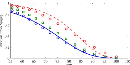
The average European values in the year 1900 are approximately also observed for England in 1850-1900 and for Sweden in 1750-1900 (see Strulik and Vollmer, 2013). The time invariance of these numbers is consistent with the general observation that adult mortality was very similar in Western Europe and did not change much before the 20th century. We thus set ϕ = 0.08 and B = 0.00018 for 1900 and earlier and ϕ = 0.11 and B = 0.00001 for the year 2000. From these values we compute the unconditional survival probability S(x) by solving ˙S(x)/S(x) = µ(x) for S(x). The result is shown in Figure 1. The solid blue line
shows survival rates in 1900, the red dashed line shows survival rates in 2000.
sur-Figure 1: Actual and Predicted Survival Probability 55 60 65 70 75 80 85 90 95 100 105 0 0.2 0.4 0.6 0.8 1 su rv iv a l p ro b S (a g e) age
Survival probabilities in Germany according to Gompertz law in 1900 (solid line) and 2000 (dashed line) and predictions by the model (dots). Squares indicate improvement of survival not originating from improved health care. See text for details.
vival probabilities provide the best fit of the actual survival probabilities in the year 1900 (given β1 = β2 = 0). The blue circles in Figure 1 show the implied survival probabilities for
χ = 0.062, α1 = 1.9, α2 = 3.8 and b = 2.5. How much of the upward shift of the survival curve during the 20th century has been caused by improved health care is a debated issue, which is not yet completely resolved. Much of the improved survival at working age was likely to be driven by improved nutrition and public health measures like sanitation and the implied reduction in the spread of diseases (McKeown, 1976; Fogel; 1994). Old age diseases like cardiovascular diseases and cancer, however, were largely unaffected by these trends and they were actually increasing during the first half of the 20th century. Moreover, the reductions in mortality at old age achieved since the 1950s can be largely attributed to medical innovations and improved medical care (Cutler and Meara, 2001). We take these stylized facts into account and assume for the benchmark run of the model that about 50 percent of improved survival of the working aged is caused by an “improved health environ-ment”, as shown by the green squares in Figure 1. It is reached by an exogenous reduction of α1 from 1.9 to 1.5, while leaving α2 unchanged. Notice that survival in retirement im-proves as well (albeit by less than 50 percent) because of the intergenerational transmission of better health as driven by path-dependency parameter b.
We assume that the remainder of the shift of the survival curve has been caused by health technology and health expenditure. To jointly calibrate technology parameters β1,
β2, and per capita health expenditure levels, we assume that h1 and h2 fulfill health budget constraint (17) and h1/h2 = 0.29 is current ratio of health care expenditure per working-aged individual to that per retiree in Germany.16 Under these assumptions, the best fit of the survival curve for the year 2000 is reached for β1 = 0.83 and β2 = 0.60. Predicted survival is shown by red circles in Figure 1. The calibrated model predicts that actual life expectancy at birth, LE as given by (13), is 78.5 years. Actually, life expectancy at birth was 78.0 years in the year 2000 (and 80.0 years in 2010, according to World Bank, 2015). Moreover, it predicts a GDP share of health care expenditure of 10.3 percent while actually it was 10.7 percent in the year 2008.
For further comparison with the actual data we computed the implied distribution of the frailty index, i.e. of the relative number of health deficits out of a long list of potential bodily impairments, conditional on age. Harttgen et al. (2013) have calculated the frailty index from the ‘Survey of Health, Ageing and Retirement in Europe’ (SHARE) data for several European countries including Germany. Estimates and predictions are shown in Figure 2. As a reading example for the left panel of Figure 2, since the maximum number of health deficits in the calibrated model is ¯n = 20, a frailty index of 0.2 means four health
deficits. The model approximates the overall distribution reasonably well. The working-aged individuals in our model are a bit too healthy when compared with 50-54 year old persons from the SHARE sample. This seems fine, however, since that cohort is already quite close to the retirement age compared to the average German worker. Unfortunately, SHARE does not provide any data for persons younger than 50. The frailty distribution of the retired population in our calibrated model corresponds very well to the actual frailty distribution of the 75-79 year olds.
Disutility of work at the extensive margin (retirement) is driven by a preference for 16We use data from the Statistical Office in Germany on health costs and population sizes split up by
age, retrieved on September 20, 2015 (https://www-genesis.destatis.de/genesis/online). Total health costs for those aged 15-64 and those aged 65+ are about EUR 116 million and 123 million, respectively. The population size of those aged 65+ relative to those aged 15-64 is about 0.31. This implies that health spending for someone aged 15-64 is less than a third than health spending for someone aged 65+.
Figure 2: The Frailty Index: Calibration vs. Estimation from SHARE Data for Germany 0 0.2 0.4 0.6 0.8 0 0.1 0.2 0.3 0.4 frailty index 0 2 4 6 0 .2 .4 .6 .8 Age 50−54 Age 75−79
Frailty index − Germany (2007)
Left: predicted probability distribution of the frailty index for working age population (solid line) and retired population (dashed line). Right: Estimated density of the frailty index for the age group 50-54 and 75 to 79.
leisure. We specify
V (R, n1) = ν· (1 + ξ · n1)· R1+1/γ, ν > 0, γ > 0, ξ≥ 0. (42)
We set γ = 0.25, which equals the Frisch elasticity of labor supply at the extensive margin, according to recent evidence (Chetty et al., 2011a,b). It turns out that the model provides considerable variation in results with respect to alternative assumptions about ξ, i.e. the influence of health on the disutility from work. We set ξ = 1 in the benchmark run and provide sensitivity analysis for smaller and larger ξ. A value of ξ of one means that individuals are willing to retire three years later for an improvement of their frailty index at retirement age from 0.1 (approximately the mode of the distribution of the frailty index in Germany at age 65) to 0.05 (i.e. a reduction in health deficits from n1 = 2 to n1 = 1 out of ¯n = 20 potential deficits).17
This leaves us with two degrees of freedom, the value of ν in disutility function V and the scale parameter A in the production technology. We pin down these parameters by
17To see this, evaluate the marginal rate of substitution between R and n given utility V , i.e. V
n/VR=
ξR(1 + ξn1)−1/(1 + 1/γ), at ξ = R = 1, n1= 2, and γ = 0.25 (subscripts on V denote partial derivatives).
This gives us Vn/VR= 1/15. Recalling that a time period of one corresponds to 45 years in our model, the
increase in retirement age which makes the individual indifferent between a reduction of one health deficit and working longer is 45/15 = 3 years.
assuming that the current social security system is constrained-optimal, i.e. that τs = 0.187
and ¯R = 1 (retirement at 65) would be selected behind the veil of ignorance given the
current public health system. This provides the estimates A = 34 and ν = 0.161. An interesting question for policy analysis to which we turn now is to determine the jointly optimal social security and health system for the current health technology (future prospects are examined in section 7).
6
Currently Optimal Health and Pension Policy
In this section we determine the currently optimal pension and health system simulta-neously, i.e. we solve the expected welfare maximization problem (29) in the calibrated model.
6.1
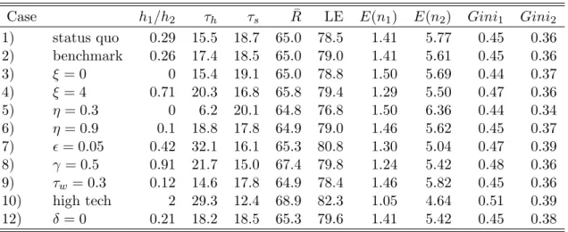
Benchmark Scenario
The first row of Table 1 displays the status quo before optimization. Results for the baseline calibration are shown in the second row (“benchmark” Case 2). The best policy is characterized by a mild increase of health expenditure as a fraction of labor income from 15.5 to 17.4 percent, i.e. by 12%. The health care improvement leads to an increase of life expectancy at birth, LE, of 0.5 years. Health spending for a younger person shall be about a fourth of the health spending for an elderly person, a mild decrease compared to the status quo. Furthermore, individuals still prefer to retire at age 65. Interestingly, the longer stay in the retirement period because of higher health expenditure (compared to the status quo) is optimal together with a mildly lower pension contribution rate, τs, from 18.7
to 18.5 percent, showing that individuals prefer a healthy life against high consumption in retirement. The notion will become more apparent in cases with larger deviations of the optimal policy from the status quo, particularly in section 7 where we analyze the implications of medical progress. It reflects the fact, emphasized by Hall and Jones (2007), that welfare is linear in the length of life but strictly concave in consumption per period.