• Aucun résultat trouvé

Sparsity-based optimization of two lifting-based wavelet transforms for semi-regular mesh compression

N/A
N/A
Protected

Academic year: 2021

Partager "Sparsity-based optimization of two lifting-based wavelet transforms for semi-regular mesh compression"

Copied!
15
0
0

Texte intégral

(1)

HAL Id: hal-00687445

https://hal.archives-ouvertes.fr/hal-00687445

Submitted on 13 Apr 2012

HAL is a multi-disciplinary open access

archive for the deposit and dissemination of

sci-entific research documents, whether they are

pub-lished or not. The documents may come from

teaching and research institutions in France or

abroad, or from public or private research centers.

L’archive ouverte pluridisciplinaire HAL, est

destinée au dépôt et à la diffusion de documents

scientifiques de niveau recherche, publiés ou non,

émanant des établissements d’enseignement et de

recherche français ou étrangers, des laboratoires

publics ou privés.

Sparsity-based optimization of two lifting-based wavelet

transforms for semi-regular mesh compression

Aymen Kammoun, Frédéric Payan, Marc Antonini

To cite this version:

Aymen Kammoun, Frédéric Payan, Marc Antonini. Sparsity-based optimization of two lifting-based

wavelet transforms for semi-regular mesh compression. Computers and Graphics, Elsevier, 2012, 36

(4), pp.272-282. �10.1016/j.cag.2012.02.004�. �hal-00687445�

(2)

Sparsity-based optimization of two lifting-based wavelet transforms for

semi-regular mesh compression

Aymen Kammoun, Fr´ed´eric Payan and Marc Antonini Laboratoire I3S, UMR CNRS - Universit´e de Nice Sophia Antipolis, France

Abstract

This paper describes how to optimize two popular wavelet transforms for semi-regular meshes, using lifting scheme. The objective is to adapt multiresolution analysis to the input mesh to improve its subsequent coding. Consider-ing either the Butterfly- or the Loop-based liftConsider-ing schemes, our algorithm finds at each resolution level an optimal prediction operator P such that it minimizes the L1-norm of the wavelet coefficients. The update operator U is then

re-computed in order to take into account the modifications to P. Experimental results show that our algorithm improves on state-of-the-art wavelet coders.

Keywords: Wavelets, Lifting scheme, Semi-regular mesh, Compression, Butterfly, Loop, Sparsity, Optimization.

1. Introduction

Wavelets have their roots in approximation theory [1] and signal processing [2] in the late eighties. Since then, wavelets are the most popular technique for rep-resenting data in a multiresolution way. They have been used for a vast number of applications: physic, biomed-ical signal analysis, image processing, and so on. But wavelets have been particularly designed for data cod-ing, because they guarantees compact representation of transformed data, and consequently high compression performances.

In computer graphics, the compact representation is not the sole attractive feature of wavelets. Indeed, current high-resolution acquisition techniques produce highly detailed and densely sampled surface meshes. Not only these massive monoresolution data are diffi-cult to handle and store, but they are also awkward for fast and progressive transmission in bandwidth-limited applications. Wavelets tackle such issues, the multires-olution structure (Figure 1) making the progressive pro-cessing easier.

A problem for applying wavelets on meshes is the ir-regular sampling (unlike still images or videos). Despite the development of wavelets for irregular meshes [3, 4], a popular solution is to remesh the input mesh semi-regularly (for instance with [5, 6, 7]) before applying

Email address:{kammoun,fpayan,am}@i3s.unice.fr

(Aymen Kammoun, Fr´ed´eric Payan and Marc Antonini)

wavelets. The principle is to resample the surface ge-ometry while providing a subdivision connectivity. The output is called a semi-regular mesh, and wavelet filter-ing is finally more efficient.

1.1. Related work

Lounsbery et al. are considered as pioneers in the development of wavelets for surface meshes of arbi-trary topological type [8]. They proposed a technique to construct wavelets from any local, stationary, contin-uous, uniformly convergent subdivision schemes such as Catmull-Clark [9], Loop [10], or Butterfly [11]. The subdivision scheme represents the synthesis filter, and the analysis filter is derived from it. Two filters are finally applied on the input mesh during analysis pro-viding respectively a mesh of low resolution (low-pass filtering), and a set of wavelet coefficients (high-pass fil-tering).

Inspired by the work of Lounsbery et al., and by the work of Donoho concerning interpolating wavelet transforms [12], Schr¨oder and Sweldens presented how building wavelets for scalar functions specifically de-fined on a sphere [13]. They are not the first construct-ing wavelets on the sphere. The pioneers are Dahlke et

al. [14], who used a tensor product basis where one

fac-tor is an exponential spline. A continuous transform and its semi-discretization have been also proposed by Free-den and Windheuser [15]. Nevertheless, the work of Schr¨oder and Sweldens in [13] is remarkable because it

(3)

Figure 1: Overview of a wavelet decomposition.

is the first showing how the lifting scheme [16] is partic-ularly relevant to construct biorthogonal wavelets with nice properties, and how the resulting wavelet filters are easy to implement (local vertex-manipulating fil-ters). Moreover, this technique is parameterization inde-pendent. Kovacevic and Sweldens then generalized the concept of wavelets for any kind of meshes [17]. They showed that the lifting scheme allows to construct filter banks and wavelets for any lattice, any dimension, and any number of primal/dual vanishing moments. They also showed that only two lifting steps are needed (pre-dict and update), but one condition is that the associated scaling functions are interpolating.

Until this work, most of wavelet transforms for semi-regular meshes were based on interpolating subdivision schemes, in particular on the Butterfly scheme. However, a Loop-based wavelet transform was proposed in 2000 by Khodakovsky et al. [18]. The approximating Loop subdivision scheme is used during synthesis as low pass reconstruction filter, whereas the associated high-pass filter is derived from it by applying a quadrature mirror construction. The draw-back of this approach arises during wavelet analysis, because filters cannot be directly applied. Contrary to wavelet transforms based on lifting scheme, the wavelet coefficients and the low resolution mesh are obtained by solving sparse linear systems depending on the two low- and high-pass reconstruction filters. In 2004, Bertram overcame this problem by proposing a biorthogonal Loop-based wavelet construction based on the lifting scheme [19]. This is also the case of Li et

al. who proposed in parallel a reversible (but unlifted)

Loop-based wavelet transform [20]. Finally, in 2008, Charina and St¨ockler proposed to tackle this drawback by using tight wavelet frames [21], which leads to the use of the same scheme during reconstruction and decomposition.

Compression allows compact storage and/or fast transmission in bandwidth-limited applications of mas-sive meshes, and many techniques have been already

proposed [22]. To our knowledge, wavelet-based coders that take semi-regular meshes as input are the most ef-ficient, because of their piecewise sampling regularity allowing efficient wavelet decomposition. We briefly present the main works in this domain.

The first wavelet-based coder (often called PGC) for semi-regular meshes was proposed by Khodakovsky et

al. [18]. This coder is based on multi-scale quadtree

structures and supports quality scalability. The authors propose a Loop-based wavelet transform (presented in previous section), but any wavelet transform could be used. A zerotree coder followed by an entropy encod-ing are applied in parallel on each component (tangen-tial and normal) of the wavelet coefficients computed in a local frame. This coder has been also proposed for

normal meshes [23]. The only difference is the choice

of the wavelet transform. The authors uses the unlifted Butterfly-based wavelet transform (i.e., without update step), optimal for this kind of meshes.

Then, several allocation techniques [24, 25, 26, 27] were proposed for improving the coding performances of the wavelet coders. The principle is to use a bit al-location process during the quantization step in order to analytically optimize the rate-distortion tradeoff, in other words, reach the maximal quality for a minimal file size (or vice versa).

Recently, a coder providing both resolution and qual-ity scalabilqual-ity was proposed by Denis et al. (2010) [28]. This coder exploits the intraband or composite statisti-cal dependencies between the wavelet coefficients. By following an information-theoretic analysis of these sta-tistical dependencies, the wavelet subbands are indepen-dently encoded using octree-based coding techniques and a context-based entropy coding. This coder pro-vides better results than PGC, and similar results with [24] that is not quality scalable.

1.2. Motivation and Contributions

One limitation of wavelets for meshes is that the structure is fixed. For instance, many wavelet coders

(4)

use the Butterfly-based scheme [13]. From a com-pression point-of-view, this wavelet is relevant for smooth surfaces because of the interpolating effect of the Butterfly scheme used as predictor, which produces small coefficients. But this scheme is less efficient for other kinds of surfaces, with high frequency variations or salient features, for instance. Finally, a wavelet changing in function of the geometric features of the input mesh could be a relevant tool. When the transforms are lifting-based, this can be finally achieved by adapting the predict and update steps [29] to the input mesh.

Therefore we propose an algorithm for optimizing two popular lifting-based wavelet transforms for semi-regular meshes: the Butterfly-based scheme [13], and the Loop-based one [19]. Our motivation is to improve the performances of the state-of-the-art wavelet coders, by adapting the multiresolution analysis tool to the fea-tures of the input mesh. The basic idea is to find, for a given semi-regular mesh, the prediction operator that maximizes the sparsity of wavelet coefficients at each level of resolution. Indeed, it is well known in informa-tion theory that maximizing the data sparsity improves the coding performances [30].

The idea of adapting the prediction step of the Butterfly-based scheme has been already introduced in [31]. The main contributions of the current paper are:

• More technical details about the optimization

algo-rithm for the Butterfly-based lifting scheme;

• A more robust method for computing the update

operator for this scheme. The reason is that the technique proposed in [31] sometimes fails be-cause of a potential null divisor;

• An extension of the optimization algorithm to the

Loop-based lifting scheme [19], by taking into ac-count the features of this scheme.

The rest of this paper is organized as follows. Section 2 introduces notions about semi-regular meshes and lift-ing scheme for semi-regular meshes. Section 3 and 4 present our contributions, respectively for the Butterfly-based and the Loop-Butterfly-based lifting schemes. Section 5 shows some experimental results, and we finally con-clude in section 6.

2. Background and notations

2.1. Semi-regular meshes

A semi-regular mesh ML is based on a mesh hierar-chy Ml (l ∈ {0, 1, ..., L}) that represents a given surface

at different levels of details, or resolutions (see Fig. 2).

M0 corresponds to the lowest resolution, and is called the base mesh. Mlis a subdivided version of Ml−1, and corresponds to lth resolution. Subdivision consists in splitting each triangle into four smaller ones by adding new vertices on each edge, and then updating their po-sition to fit as closely as possible to the original surface.

ML corresponds to the highest resolution of the given surface.

Figure 2: Structure of a semi-regular mesh.

2.2. Wavelet filtering for semi-regular meshes

Let us denote Vjthe set of vertices of a given mesh

Mj, defined by their position in the Euclidean space. Applying a wavelet transform to Mjgives one mesh of lower resolution Mj−1defined by a set of vertices Vj−1, and a set Cjof 3D wavelet coefficients. Figure 3 illus-trates this decomposition.

ࡹ௝ ௝ିଵ

࡯௝

LP

HP

Figure 3: Wavelet analysis of a semi-regular mesh. Mjis transformed

into a mesh Mj−1of lower resolution and a set Cjof coefficients (rel-ative to the red dots).

2.3. Lifting scheme

An efficient tool for building wavelet transforms is the lifting scheme [16]. The main feature of the lifting scheme is that all constructions are derived in the spatial domain while the traditional approach relies on the frequency domain. The lifting scheme has several advantages [32], in particular for surface meshes. For example, the lifting scheme i) leads to algorithms that can be generalized to complex geometric situations; ii) allows in place transformation, reducing the nec-essary amount of memory; iii) leads to a reversible

(5)

implementation (analysis/synthesis), faster than im-plementation based on filter banks. Nevertheless, the lifting scheme has few drawbacks. For instance, the sta-bility of the transform is not guaranteed by construction. The canonical lifting scheme (Figure 4) is based on three steps:

• Split. We split the original data set into two

sub-sets. In our context, the vertices Vjare split into two subsets V0j and V1j(green and red dots on the figure 3);

• Predict. We take as input the subset V0jand predict the positions of the vertices V1j by using an oper-ator P, so that V1j = P(V0j). The prediction errors are the wavelet coefficients Cj;

• Update. We take as input Cjand modify the posi-tions of the vertices V0jby using an operator U and a gain (×2). We finally obtain the low resolution mesh Mj−1, defined by a set of vertices Vj−1. For the synthesis, we only have to reverse the order and the sign of the different steps (Figure 5).

+

Split

-P

U

+

x2

௝ ࢂ௝ ࢂ௝ ࢂ௝ିଵ ࡯௝

Figure 4: Analysis lifting scheme for semi-regular meshes.

/2

-U

+

+

+P

Merge ௝ ࢂ௝ ࢂ௝ ࢂ௝ିଵ ࡯௝

Figure 5: Synthesis lifting scheme for semi-regular meshes.

3. Adaptive Butterfly-based lifting scheme

In this section we present our optimization algorithm for adapting the Butterfly-based lifting scheme to the input mesh. This algorithm consists in finding for each resolution the optimal operators P such as the sparsity of the wavelet coefficients is maximized [31]. This algo-rithm produces new stencils for each level of resolution. Our wavelet coefficients are vector valued (three co-ordinates x, y, and z) and represented in local frames de-pending on the surface normals [18]. When using local frames, the state of the art wavelet coders consider the tangential components (x and y), and the normal com-ponents (z) separately. We thus propose to compute two prediction operators, Pxy and Pz, according to the two sets of components. The algorithm presented below will be used to get Pxy and in parallel Pz. For the conve-nience of the readers, we define hereinafter P for both

Pxyand Pz.

3.1. Optimization of the operator P

The predict step is based on the modified Butterfly

scheme [33] defined by two stencils: the regular and the

irregular (Figure 6).

• For a given vertex v ∈ V1j, the regular stencil is used when its direct neighbors belonging to V0jare regular (i.e., valence 6).

• The irregular stencil is chosen for any other case.

(a) Regular stencil. (b) Irregular stencil. Figure 6: Prediction stencils of the Butterfly-based lifting scheme.

Our algorithm optimizes only the regular stencil, be-cause there are too many configurations for the irregular one (depending on the valence of the neighbors). Opti-mizing all the potential irregular stencils may produce a critical amount of side information (necessary for re-constructing the meshes during synthesis).

Considering the level of resolution j, the set Cj of wavelet coefficients is computed by using

(6)

In order to increase the coding performances, we want Cjto become as sparse as possible. One solution proposed in the literature is to minimize the L1-norm of

this set [34]. So, maximizing the sparsity can be seen as the minimization problem

min

αj

||V1j− Pαj(V

j

0)||1, (2)

where αjdefines the weights of P for the level of reso-lution j.

To solve this problem, we define the unknown vec-tor x =0j, α1j, . . . , α9jT containing the ten weights of

P, and N(v) the set of ten neighbor vertices of Vj0 and depending on the regular stencil. We now define the matrix A of dimension (nr× 10)

A =hN(V1j(0)) ; N(V1j(1)) ; . . . N(V1j(nr− 1))

i ,(3) where nr is the number of vertices of V

j

1 on which the

regular stencil is applied at this resolution. We then de-fine the vector b

b =V1j(0), V1j(1), . . . V1j(nr− 1)T. (4)

Finally, (2) can be solved by minimizing one function

f defined by f : R

10 7−→

R

x 7−→ f (x) = ||Ax − b||1. (5)

Since the Butterfly scheme is symmetric, we can write

α0 = α1

α2 = α3

α4 = α5= α6 = α7

α8 = α9. (6)

Finally, the function f has only four unknown values (α0, α2, α4and α8) and can be written as following

f : R

4 7−→

R

x 7−→ f (x) = ||Ax − b||1. (7)

This function f is convex (see Appendix A for de-tails) and bounded by 0, so f has a unique and global minimum. To find this minimum, we use the Nelder-Mead simplex algorithm [35], but other algorithms may be used. The proposed optimization algorithm is ap-plied to each level of resolution, successively from the highest to the lowest.

3.2. Computation of the new operator U

Considering the same level of resolution j and the canonical lifting scheme (Figure 4), the set of vertices Vj−1is obtained by using

Vj−1= 2 × (V0j+ U(Cj)), (8)

where U is the update operator depending on a weight

γand associated to the stencil given by Figure 7.

ߛ

ߛ ߛ

ߛ ߛ ߛ

Figure 7: Update stencil of the Butterfly-based lifting scheme. When the prediction P is based on a subdivision oper-ator, the update U, that depends on P, has to be chosen for obtaining vanishing moments [32]. P being modi-fied at each level of resolution by the optimization al-gorithm, the weight γ of the update operator U has to be recomputed. In this work, we choose to compute

γsuch as to preserve the average between Vjand Vj−1. Contrary to [31], we prefer using the robust method pro-posed in [32]. The principle is to put all the vertices of Vj−1and all the coefficients of Cjto zero, except one coefficient of Cjput to 1 (see Figure 8).

Figure 8: Method for computing γ. The orange dot (a) represents the only non null coefficient; the green dots (b) represent the two sole vertices of Vj−1with non null values after synthesis; the red dots rep-resent the 43 vertices of Vjwith non null values after synthesis.

We apply the synthesis filters, and obtain Vj. A ma-jority of the resulting vertices has null coordinates, ex-cept 43 over which the non null coefficient Cjspread. These vertices are also shown on Figure 8. The value associated to each vertex are given by Table 1.

(7)

index count value a 1 1 -2γα0 b 2 −γ c 4 −γ(α0+ α2) d 4 −γ(α0+ α4) e 2 −γ(α0+ α8) f 4 −γ(α2+ α4) g 4 −γα2 h 4 −γα4 i 4 −γ(α4+ α8) j 4 −γα8 k 4 −γα4 l 4 −γα4 m 2 −γα8

Table 1: Values of the 43 non null vertices of Vjobtaining after

syn-thesis from only one non-null coefficient of Cj.

In this case, the average of Vjis equal to 1

43(1 − 2γ − 12γα0− 12γα2− 24γα4− 12γα8) .(9) Since the average of Vj−1is null, equation (9) has to be also null. We finally obtain

γ = 1

2 + 12α0+ 12α2+ 24α4+ 12α8

. (10)

3.3. Validation of the algorithm

To verify the efficiency of our optimization algorithm, we compare the L1-norm of the wavelet coefficients

obtained with the state of the art Butterfly-based lift-ing scheme (Classical), and with the proposed adaptive scheme (Optimized I). The results for Vase Lion are pre-sented in Table 2.

Classical Optimized (I) Optimized (II)

res TC NC TC NC TC NC 1 83.76 132.21 84.41 126.40 83.80 125.18 2 62.32 134.32 62.21 125.53 62.10 125.50 3 45.80 126.92 45.10 116.87 45.08 116.88 4 31.53 77.88 29.94 69.53 29.93 69.51 5 21.08 42.15 20.22 39.22 20.22 39.21 6 13.81 26.10 13.50 25.78 13.50 25.78

Table 2: L1-norm of the tangential and normal components (TC and NC) of the wavelet coefficients obtained with the state of the art Butterfly-based lifting scheme (Classical) and with our adaptive scheme (Optimized (I)) for Vase Lion. Optimized (II) is our adaptive scheme without constraint of symmetry. res is the level of resolution.

We observe that the L1-norm of each subset is

glob-ally lower with our adaptive scheme. Similar results are obtained for all the experimented models, proving that

our algorithm works well. Nevertheless, for few mod-els (e.g. Vase Lion, Table 2), our algorithm does not decrease the L1-norm of the tangential components of

lowest resolution. This issue sometimes arises, only at this resolution, when a majority of vertices are irregular and requires the irregular stencil. In this specific case, our optimization algorithm may not be effective at this resolution but remains efficient for the other resolutions. We also studied the influence of the constraint of symmetry (6) required by the prediction stencil. The column Optimized (II) presents the results of our algo-rithm without this constraint. We observe that the re-sults are similar. The constrained optimization process being three times faster (see Table 3), we finally retain this variant for the experimentations (Section 5).

4. Adaptive Loop-based lifting scheme

As introduced in Section 1, we now expand our optimization technique to the Loop-based lifting scheme [19]. This transform, illustrated by figure 9, dif-fers from the canonical lifting scheme.

+

Split

-P

U

2

+

-U

1

+

௝ ࢂ௝ ࢂ௝ ࢂ௝ିଵ ࡯௝ Figure 9: Analysis Loop-based lifting scheme[19]. The main features of this scheme are:

• a prediction operator P depending on two weights ρ0and ρ1(see Figure 10(a));

• an update operator U1 applied before the predict

step depending on a weight δ (see Figure 10(b)). A gain1β (that depends on the valence of the vertices) is also applied;

• a second operator U2depending on weights ω (see

Figure 10(c)). This step is applied to obtain a biorthogonal wavelet transform.

Note that the two update filters depend on the weights ρ of P.

(8)

Model # resolution # vertices Optimized (I) Optimized (II)

Bimba 7 999426 79 207

Rabbit 6 163842 13 34

Vase Lion 6 675842 55 141

Table 3: Computation time (in seconds) for optimizing the Butterfly-based scheme (Matlab implementation).

ߩ଴ ߩ଴ ߩଵ ߩଵ (a) Prediction. ߜ ߜ ߜ ߜ ߜ ߜ (b) First update. ߱ଵ ߱଴ ߱ଶ ߱ଷ (c) Second update. Figure 10: Stencils of the Loop-based lifting scheme.

4.1. Optimization of the operators P and U1

We still minimize the L1-norm of the wavelet

coef-ficients at each level of resolution, but the tangential and the normal components are not considered sepa-rately, unlike the Butterfly case. Indeed, if two predic-tion operators Pxyand Pzare computed (for the tangen-tial and the normal components), we obtain two sets of wavelet functions for each vertex, and the orthogonal-ization done by the update filter U2becomes impossible

[19]. Thus, at each level of resolution, the algorithm takes the set of vector valued coefficients as input, and gives only one optimized P.

The predictor depends on two parameters ρ0 and

ρ1. So, the minimization problem for this scheme is

min{ρ0,ρ1}||C j||

1. But, contrary to the Butterfly-based

scheme, the coefficients are obtained after two steps, U1

and P. The prediction operator P and the first update operator U1 have to be optimized simultaneously, and

the minimization problem becomes

min {ρ0,ρ1} ||V1j− P         V0j− U1  V1j β         ||1. (11)

When minimizing this function, the weight δ of U1and

βmust be recomputed at each iteration, since they de-pend on ρ0and ρ1. For a vertex v of V0j, they are

formu-lated by β(n) = 1 1 − ρ0 ρ0+ 2ρ1cos 2π n !2 , (12) δ(n) = 1 − β(n) n . (13)

where n is the valence of v at this resolution.

To find the optimal weights ρ∗ at each resolution,

we use the same algorithm than for the Butterfly-based scheme, i.e., the Nelder-Mead simplex algorithm [35]. To respect the constraint of the Loop subdivision scheme, we assume that the sum of the four weights of the prediction stencil is equal to one.

4.2. Computation of the new operator U2

Now we have to modify the second update operator

U2 that depends on ω. In [19] the author details how

computing ω in function of the weights ρ, to finally get a biorthogonal wavelet scheme. Since our algorithm modifies the predictor at each resolution level, we also have to compute new weights ω at each resolution level. As explained in [19], we have to solve Aω = b, where

A is a symmetric 4 × 4 matrix A =               a00a01a02a03 a10a11a12a13 a20a21a22a23 a30a31a32a33               ,

and b is a 4 × 1 matrix defined by b = [b0 b1 b2b3]T.

Finally, the key problem is to compute ai j and bi that depend on ρ. Once these weights computed, the weights

ωrelative to each vertex of each resolution are obtained

by computing ω = A−1b. For the convenience of the

readers, details of how computing the terms ai j and bi can be found in Appendix B.

4.3. Validation of the method

To validate our optimization algorithm for the Loop-based lifting scheme, we compared the L1-norm of the

wavelet coefficients obtained with the classical scheme (Classical), and with our adaptive scheme (Optimized), for several models. The results for Joan of Arc are pre-sented in Table 4. We observe that our optimization algorithm is also efficient with the Loop-based lifting scheme, since the L1-norm values are always

(9)

Classical Optimized res TC NC TC NC 1 13.63 15.51 8.05 11.65 2 16.49 17.24 13.18 14.96 3 16.02 16.85 13.78 15.37 4 15.89 16.91 14.74 16.06 5 12.70 13.82 12.56 13.80

Table 4: L1-norm of the tangential and normal components (TC and

NC) of the wavelet coefficients obtained with the state of the art

Loop-based lifting scheme (Classical) and with our adaptive scheme

(Opti-mized) for Joan of Arc. res is the level of resolution.

Wavelet Transform Quantizer Entropy Coding Connectivity Coding Semi-regular Mesh ntropy Specific Bitrate Compressed File +

Figure 11: Overview of wavelet coder for semi-regular meshes.

5. Application to the geometry compression

To evaluate if our technique improves the coding of the semi-regular meshes, we now include our adaptive transform into a wavelet coder.

The main steps of a wavelet coder (Figure 11) are: 1. Wavelet transform. This stage provides the

sub-bands of 3D wavelet coefficients and the lowest resolution mesh.

2. Connectivity coder. The connectivity of the low-est resolution mesh is lossless encoded (for in-stance, with [36]).

3. Quantizer. The subbands of coefficients are quan-tized so that the minimum reconstruction error is introduced, according to a specific bitrate.

4. Entropy coding. The quantized data are entropy coded.

We experiment two coders. The first one is called PGC [18]. This is the first wavelet coder for semi-regular meshes (see section 1.1), and the most popular. The sec-ond one is the coder of [24, 25], called hereinafter EDQ. This coder includes a bit allocation that minimizes the reconstruction error by computing the optimal quanti-zation steps {qi} of each subband for a specific bitrate

Rtarget. This allocation is done by minimizing the La-grangian criterion

Jλ({qi}) = DT({qi}) + λ(RT({qi}) − Rtarget), (14) where DT is the mean square error between the quan-tized and the original vertices, and RT is the bitrate.

Assuming that the distribution of the tangential and the normal components can be modeled by a Generalized Gaussian Distribution, theoretical models are used for estimating the bitrate and the distortion of each sub-band. We choose to experiment this coder because it is model-based. We would like to verify if our optimiza-tion algorithm is also relevant for such a coder, in other words if our algorithm does not drastically change the statistical properties of the wavelet coefficients.

5.1. Results for the Butterfly-based scheme

Tables 5 to 10 show the values of PSNR and RMS for three models (Vase Lion, Bimba and Rabbit), analyzed with the classical or with our adaptive Butterfly-based scheme, and then compressed with PGC or with EDQ.

The RMS corresponds to the surface-based Root Mean Square error, computed between the original ir-regular mesh and the reconstructed semi-ir-regular with MESH tools [37]. The PSNR is given by

PS NR(dB) = 20log10

BB

RMS, (15)

with BB the length of the bounding box diagonal. The bitrates are given in bits per irregular vertex (b/iv). For the adaptive scheme, the bitrate includes the set of opti-mized weights, needed for decoding.

Classical Optimized (I) Gain

Bitrate RMS PSNR RMS PSNR RMS 2.50 5.49 68.03 5.19 68.51 5.37% 3.50 4.08 70.60 3.82 71.16 6.29% 5.50 2.70 74.20 2.57 74.62 4.75% 9.00 1.84 77.52 1.78 77.79 3.00% 11.00 1.58 78.86 1.53 79.14 3.13% 13.00 1.46 79.54 1.40 79.91 4.22%

Table 5: Coding results for Vase Lion when using the Butterfly-based schemes and PGC. The RMS is in multiples of 10−4.

Classical Optimized (I) Gain

Bitrate RMS PSNR RMS PSNR RMS 1.75 10.21 81.91 10.14 82.38 5.28% 2.50 8.43 85.04 8.24 85.24 2.20% 3.50 6.36 87.79 6.31 87.56 0.77% 5.50 4.76 90.01 4.65 90.21 2.31% 9.00 3.76 92.06 3.70 92.18 1.42% 11.00 3.46 92.78 3.43 92.85 0.87%

Table 6: Coding results for Bimba when using Butterfly-based schemes and PGC. The RMS is in multiples of 10−5.

(10)

Classical Optimized (I) Gain Bitrate RMS PSNR RMS PSNR RMS 1.75 7.81 81.53 7.66 81.70 2.01% 2.50 6.41 83.25 6.38 83.29 0.43% 3.50 5.69 84.29 5.59 84.43 1.65% 5.50 5.04 85.33 4.99 85.43 1.06% 9.00 4.61 86.11 4.59 86.15 0.46% 13.00 4.48 86.35 4.48 86.36 0.14%

Table 7: Coding results for Rabbit when using Butterfly-based schemes and PGC.The RMS is in multiples of 10−6.

Classical Optimized (I) Gain

Bitrate RMS PSNR RMS PSNR RMS 2.58 5.06 68.73 4.83 69.14 4.68% 3.51 3.87 71.07 3.78 71.27 2.33% 5.33 2.78 73.92 2.71 74.17 2.77% 8.90 1.78 77.79 1.71 78.15 4.01% 10.78 1.62 78.63 1.53 79.11 5.34% 12.70 1.45 79.56 1.40 79.88 3.60%

Table 8: Coding results for Vase Lion when using Butterfly-based schemes and EDQ. The RMS is in multiples of 10−4.

Classical Optimized (I) Gain

Bitrate RMS PSNR RMS PSNR RMS 1.55 10.39 80.70 10.29 81.36 7.33% 2.17 9.86 83.68 9.21 84.27 6.58% 3.03 7.03 86.62 6.87 86.82 2.23% 4.75 5.15 89.32 5.02 89.54 2.42% 7.85 3.94 91.64 3.90 91.74 1.09% 9.60 3.62 92.38 3.55 92.54 1.90%

Table 9: Coding results for Bimba when using Butterfly-based schemes and EDQ. The RMS is in multiples of 10−5.

Classical Optimized (I) Gain

Bitrate RMS PSNR RMS PSNR RMS 1.07 9.96 79.42 9.79 79.573 1.72% 1.89 7.12 82.34 7.03 82.450 1.23% 2.63 6.45 83.19 6.39 83.277 1.00% 3.65 5.46 84.64 5.44 84.670 0.40% 10.20 4.51 86.30 4.50 86.25 0.29%

Table 10: Coding results for Rabbit when using Butterfly-based schemes and EDQ. The RMS is in multiples of 10−6.

Globally the proposed adaptive scheme improves the coding whatever the coder. The maximum gain is 6.29% for Vase Lion, 7.33% for Bimba, and 2.01% for

Rab-bit. The most significant gains are obtained for Vase

Lion and Bimba, in particular at low and medium bi-trates, where there is a room for improvement. The gain is lower for Rabbit, even negligible at some bi-trates. These results confirm our assumptions: the more the surface has important high frequency variations, the more our adaptive transform is efficient.

In addition, Figure 12 show the visual benefits of the proposed Butterfly-based technique. This figure shows the distribution of the reconstruction error of Vase Lion, analyzed with the classical transform and with the adap-tive transform (compressed with EDQ). One can argue that our adaptive wavelet transform tends to better pserve the high frequency details of the non-smooth re-gions, such as the mane. On the other hand, the classical transform seems to introduce less errors on smooth re-gions, such as the muzzle. These results confirm the fact that our adaptive transform is better suited for non-smooth regions. Thus, it could be interesting in the fu-ture to combine the two transforms in a region-based wavelet coding scheme. For instance, after using a seg-mentation technique sharing the mesh in two regions (smooth vs detailed), we could analyze them separately (smooth region = classical transform, detailed region = adaptive transform). The coding gain should be superior and the visual quality better.

We also compare the efficiency of the two transforms applied on meshes with salient features, for which the classical Butterfly-based scheme is generally less effi-cient. Figure 13 shows that our adaptive scheme tends to further preserve the salient features of Knot.

5.2. Results for the Loop-based scheme

Tables 11 to 13 gives the PSNR and RMS for Vase Lion, Bimba and Rabbit analyzed with the classical or with the adaptive Loop-based scheme, and then com-pressed with PGC. Our optimization algorithm also im-proves the coding performances when the Loop-based is used. Globally the gain is even higher than with But-terfly. The maximum gain is 19.55% for Vase Lion, 19.73% for Bimba, and 6.31% for Rabbit, still at low bitrates.

One drawback of the classical Loop-based wavelet is to create distorted low resolution meshes, in particular when the input is complex. By comparing the resolu-tions of several models, we observe that the proposed adaptive scheme creates low resolution meshes less dis-torted than with the original scheme. Figure 14 illus-trates this fact. This is a very interesting feature, which

(11)

(a) Classical wavelet. (b) Adaptive wavelet.

Figure 12: Distribution of the reconstruction error of Vase Lion, analyzed with the classical and with the adaptive Butterfly-based scheme (com-pressed with EDQ). The color corresponds to the magnitude of the distance point-surface computed between the original mesh and the com(com-pressed (MESH tools).

(a) Original Knot. (b) A salient feature (zoom).

(c) Classical wavelet transform. (d) Adaptive wavelet transform. Figure 13: Salient features of compressed models tend to be better preserved with our adaptive Butterfly-based scheme.

Classical Adaptive Gain

Bitrate RMS PSNR RMS PSNR RMS

2.5 10.53 59.13 10.39 59.95 9.01%

5.5 6.99 65.92 5.63 67.81 19.55%

9 4.47 69.80 4.43 69.89 1.08%

11 3.35 72.30 3.26 72.54 2.70%

Table 11: Coding results for Vase Lion when using Loop-based schemes and PGC. The RMS is in multiples of 10−4.

Classical Adaptive Gain

Bitrate RMS PSNR RMS PSNR RMS

1 4.96 69.64 3.98 71.55 19.73%

1.75 2.71 74.90 2.39 76.00 11.86%

3.5 1.44 80.36 1.41 80.55 2.17%

9 0.78 85.76 0.77 85.86 1.16%

Table 12: Coding results for Bimba when using Loop-based schemes and PGC. The RMS is in multiples of 10−4.

(12)

(a) Left: original model; top: our adaptive scheme; bottom: the classical scheme.

(b) Left: original model; top: our adaptive scheme; bottom: the classical scheme.

(13)

Classical Adaptive Gain Bitrate RMS PSNR RMS PSNR RMS 1.75 10.01 79.34 9.54 79.80 5.18% 5.5 5.50 84.58 5.47 84.63 0.63% 9 4.79 85.79 4.79 85.79 0.38% 11 4.60 86.13 4.59 86.16 0.33%

Table 13: Coding results for Rabbit when using Loop-based schemes and PGC. The RMS is in multiples of 10−6.

can be exploited in a progressive application (transmis-sion, coding, and so on).

6. Conclusion and future works

We described an algorithm for optimizing two wavelet transforms for semi-regular meshes based on lifting scheme: the Butterfly- and the Loop-based trans-form. Our optimization consists in computing a predic-tion operator P that maximizes the sparsity of wavelet coefficients (by minimizing the L1-norm) for

improv-ing the subsequent codimprov-ing. This optimization is done at each level of resolution during the analysis. Exper-imental results show that our optimization algorithm improves significantly the coding of non-smooth mod-els whatever the wavelet transform used. Visually, the adaptive Butterfly-based scheme also tends to further preserve the regions of high frequency details and the salient features. Finally, The Loop-based scheme cre-ates low resolution meshes less distorted than the origi-nal transform, which is very interesting for progressive applications.

For the future, a thorough study of the statistics of the coefficients could be relevant to know how these lifting schemes can be further improved, and to develop new minimization criteria. In parallel, an in-depth evalua-tion of the performances of the algorithm in funcevalua-tion of the input mesh could be also interesting. Another promising work could be the development of a region-based analysis for complex models. As proposed in the experimental section, it could be interesting to adapt the filters to several regions of the input, in function of the high frequency details (classical/adaptive transform for smooth/non smooth region for instance). Such an ap-proach should improve the global quality of the encoded meshes.

Acknowledgments

The original (irregular mesh) Vase Lion model is courtesy of SenSable Technologies. The original Joan

of arcmodel is courtesy of I3S Laboratory. The

origi-nal Bimba model is courtesy of IMATI and INRIA. The original Rabbit model is courtesy of Cyberware. All models are remeshed with Trireme [6]. We are particu-larly grateful to Igor Guskov for providing us with his executable (Trireme). We also want to acknowledge the anonymous reviewers for their comments which permit-ted us to improve the quality of this paper.

Appendix A. Convexity of the function f

This section shows that the function f developed for improving the Butterfly-based lifting scheme is convex (see Section 3). We recall that the function f is given by

f : R 10 7−→ R x 7−→ f (x) = ||Ax − b||1, with x =0j, α0j, α2j, α2j, α4j, α4j, α4j, α4j, α8j, α8jT.

By definition, the function f can be written as:

f (x) = nr−1 X i=0 |Aix − bi|, = nr−1 X i=0 gi(x),

where Aiare the rows of A, biare the values of b, and

nris the number of vertices of V1j on which the regular stencil is applied at this level of resolution. Considering (x,y) ∈R

10, and λ ∈ [0, 1], we get

gi(λx + (1 − λ)y) = |Ai(λx + (1 − λ)y) − bi|, = |λAix + (1 − λ)Aiy − bi|, = |λ(Aix − bi) + (1 − λ)(Aiy − bi)|,

|λ(Aix − bi)| + |(1 − λ)(Aiy − bi)|.

λ ∈[0, 1], so λ and (1−λ) are positive. We can deduce that

gi(λx + (1 − λ)y) ≤ λ|Aix − bi| + (1 − λ)|Aiy − bi|,

and finally:

gi(λx + (1 − λ)y) ≤ λgi(x) + (1 − λ)gi(y). Thus, the function gi is convex. Since the objective function f is a sum of gi, f is also convex.

(14)

Appendix B. Computation of ai jand bi

This section gives details about the computation of the terms ai j and bineeded to find the weights ρ of the operator U2of the Loop-based lifting scheme (see

Sec-tion 4.2).

The final goal is to solve Aω = b, where A is a symmet-ric 4 × 4 matrix A =               a00a01a02a03 a10a11a12a13 a20a21a22a23 a30a31a32a33               ,

and b is a 4 × 1 matrix b = [b0 b1 b2 b3]T. ai j and bi

are defined by the inner products ai j =< φi, φj >and

bi=< ψl, φi>, with φithe ithscaling function (i = 0..4) of the Loop transform, and ψlthe lazy wavelet. To ex-plain how computing ai jand bi, we give the examples of

b1=< ψl, φ1>and a11 =< φ1, φ1>. Figure B.15 shows

the discrete scaling function φ1 and the lazy wavelet,

with the associated parameters. Note that the ith scal-ing function φiis associated with the weight ωi(Figures 10(c) and B.16). By superposing those two stencils and computing the discrete inner product, we can easily con-clude that b1is equal to γ0δ0+ α1δ1+ ρ0, where

αi = ρ0+ ρ0+ 2ρ1cos 2π ni !2 , βi = 1 1 − ρ0 (αi− ρ0) , γi = 1 − αi ni , δi = 1 − βi ni ,

nibeing the valence of the associated vertex. Similarly, the computation of a11 can be done by superposing the

stencil of φ1on itself, and we obtain γ02+ α 2 1+ γ 2 2+ γ 2 3+ (n1− 3)γ26+ n1(ρ20+ ρ 2

1). Notice that, as Bertram in [19],

we consider that the vertices of the scaling functions that are not on the Loop stencil (blue dots on figure B.16) are regular (valence 6). Therefore their value is equal to γ6

on Figure B.15.

By following the same method on all the ai jand bi, we finally obtain for A

a00 = α20+ γ 2 1+ γ 2 2+ γ 2 3+ (n0− 3)γ26+ n0(ρ20+ ρ 2 1) a01 = a10 = α0γ0+ γ1α1+ γ22+ γ 2 3+ ρ 2 0+ 4ρ0ρ1 a02 = a20 = α0γ0+ γ21+ γ2α2+ γ62+ ρ 2 0+ 4ρ0ρ1 a03 = a30 = α0γ0+ γ21+ γ 2 6+ γ3α3+ ρ20+ 4ρ0ρ1 a11 = γ02+ α 2 1+ γ 2 2+ γ 2 3+ (n1− 3)γ26+ n1(ρ20+ ρ 2 1) ߙଵ ߛ଴ ߛଶ ߛ଺ ߛ଺ ߛଷ ߩ଴ ߩ଴ ߩ଴ ߩ଴ ߩ଴ ߩଵ ߩଵ ߩଵ ߩଵ 1 ߜ଴ ߜଵ

Figure B.15: Discrete scaling function φ1(left) and Lazy wavelet ψl

(right) of the Loop-based scheme.

߶଴

߶ଵ

߶ଷ

߶ଶ

߰௟

Figure B.16: Position of the four scaling functions and the lazy wavelet for the Loop-based prediction stencil.

a12 = a21= γ20+ α1γ1+ γ2α2+ γ26+ ρ 2 0+ 4ρ0ρ1 a13 = a31= γ20+ α1γ1+ γ62+ γ3α3+ ρ20+ 4ρ0ρ1 a22 = γ20+ γ21+ α22+ (n2− 2)γ62+ n2(ρ20+ ρ21) a23 = a32= γ20+ γ 2 1+ ρ 2 1 a33 = γ20+ γ 2 1+ α 2 3+ (n3− 2)γ62+ n3(ρ20+ ρ 2 1).

Similarly, we also obtain

b0 = (α0δ0+ γ1δ1+ ρ0)

b1 = (γ0δ0+ α1δ1+ ρ0)

b2 = b3= (γ0δ0+ γ1δ1+ ρ1).

References

[1] I. Daubechies, Orthonormal bases of compactly supported wavelets, Communications on Pure and Applied Mathematics 41 (1988) 909–996.

[2] S. Mallat, A theory for multiresolution signal decomposition: the wavelet representation, IEEE Transactions on Pattern Anal-ysis and Machine Intelligence 11 (7) (1989) 674–693. [3] I. Guskov, W. Sweldens, P. Schr¨oder, Multiresolution signal

pro-cessing for meshes, in: A. Rockwood (Ed.), SIGGRAPH ’99: Proceedings of the 26th annual conference on Computer graph-ics and interactive techniques, Addison Wesley Longman, 1999, pp. 325–334.

[4] S. Valette, R. Prost, A wavelet based compression scheme for triangle meshes : Wavemesh, IEEE Transactions on Visualiza-tion and Computer Graphics 10 (2) (2004) 123–133.

(15)

[5] I. Friedel, P. Schr¨oder, A. Khodakovsky, Variational normal meshes, ACM Transactions on Graphics 23 (4) (2004) 1061– 1073. doi:http://doi.acm.org/10.1145/1027411.1027418. [6] I. Guskov, Manifold-based approach to semi-regular

remeshing, Graphical Models 69 (1) (2007) 1–18.

doi:http://dx.doi.org/10.1016/j.gmod.2006.05.001.

[7] A. Kammoun, F. Payan, M. Antonini, Adaptive semi-regular remeshing: A voronoi-based approach, in: Proceedings of IEEE international workshop on MultiMedia Signal Processing, Saint-Malo, France, 2010, pp. 350–355.

[8] M. Lounsbery, T. D. DeRose, J. Warren, Multiresolution analy-sis for surfaces of arbitrary topological type, ACM Transactions on Graphics 16 (1) (1997) 34–73.

[9] E. Catmull, J. Clark, Recursively generated B-spline surfaces on arbitrary topological meshes, Computer-aided Design 10 (1978) 350–355. doi:10.1016/0010-4485(78)90110-0.

[10] C. Loop, Smooth subdivision surfaces based on triangles, Mas-ter’s thesis, University of Utah (1987).

[11] N. Dyn, D. Levin, J. Gregory, A butterfly subdivision scheme for surface interpolation with tension control, ACM Transactions on Graphics 9 (2) (1990) 160–169.

[12] D. L. Donoho, Interpolating wavelet transforms, Preprint, De-partment of Statistics, Stanford University (1992).

[13] P. Schr¨oder, W. Sweldens, Spherical wavelets: efficiently rep-resenting functions on the sphere, in: Proceedings of the 22nd annual conference on Computer graphics and interactive tech-niques, SIGGRAPH ’95, ACM, New York, NY, USA, 1995, pp. 161–172.

[14] S. Dahlke, W. Dahmen, I. Weinreich, E. Schmitt, Multiresolu-tion analysis and wavelets on s2 and s3, Numerical funcMultiresolu-tional analysis and optimization 16 (1,2) (1995) 19–41.

[15] W. Freeden, U. Windheuser, Spherical wavelet transform and its discretization, Advances in Computational Mathematics 5 (1) (1996) 51–94.

[16] W. Sweldens, The lifting scheme: A construction of second generation wavelets, SIAM Journal on Mathematical Analysis 29 (2) (1998) 511–546.

[17] J. Kovacevic, W. Sweldens, Wavelet families of increasing order in arbitrary dimensions, IEEE Transactions on Image Processing 9 (3) (2000) 480–496.

[18] A. Khodakovsky, P. Schr¨oder, W. Sweldens, Progressive geom-etry compression, in: SIGGRAPH’00 Proceedings of the 27th annual conference on Computer graphics and interactive tech-niques, ACM Press/Addison-Wesley Publishing Co., 2000, pp. 271–278.

[19] M. Bertram, Biorthogonal loop-subdivision wavelets, Comput-ing 72 (1-2) (2004) 29 – 39.

[20] D. Li, K. Qin, H. Sun, Unlifted loop subdivision wavelets, Pacific Conference on Computer Graphics and Applications 0 (2004) 25–33.

[21] M. Charina, J. St¨ockler, Tight wavelet frames for subdivision, Journal of Computational and Applied Mathematics 221 (2) (2008) 293–301.

[22] P. Jingliang, K. Chang-Su, C.-C. J. Kuo, Technologies for 3D mesh compression: A survey, Journal of Visual Communication and Image Representation 16 (2005) 688–733.

[23] A. Khodakovsky, I. Guskov, Compression of normal meshes, in: Geometric Modeling for Scientific Visualization, Springer-Verlag, 2003, pp. 189–206.

[24] F. Payan, M. Antonini, An efficient bit allocation for compress-ing normal meshes with an error-driven quantization, Elsevier Computer Aided Geometry Design 22 (5) (2005) 466–486. [25] F. Payan, M. Antonini, Mean square error approximation for

wavelet-based semiregular mesh compression, IEEE Transac-tions on Visualization and Computer Graphics (TVCG) 12 (5)

(2006) 649–657.

[26] J.-Y. Sim, C.-S. Kim, C. J. Kuo, S.-U. Lee, Normal mesh com-pression based on rate-distortion optimization, in: Proceedings of the IEEE Workshop on MultiMedia Signal Processing, 2002, pp. 13–16.

[27] S. Lavu, H. Choi, R. Baraniuk, Geometry compression of nor-mal meshes using rate-distortion algorithms, in: Proceedings of the Eurographics/ACM SIGGRAPH symposium on Geometry processing, Vol. 43, 2003, pp. 52–61.

[28] L. Denis, S. M. Satti, A. Munteanu, J. Cornelis, P. Schelkens, Scalable intraband and composite wavelet-based coding of semiregular meshes, IEEE Transactions on Multimedia 12 (8) (2010) 773–789.

[29] G. Piella, H. J. A. M. Heijmans, H. J. A. M. Heijmans, Adaptive lifting schemes with perfect reconstruction, IEEE Transactions on Signal Processing 50 (2001) 1620–1630.

[30] S. Mallat, A wavelet tour of signal processing, Academic Press, 1998.

[31] A. Kammoun, F. Payan, M. Antonini, Optimized butterfly-based lifting scheme for semi-regular meshes, in: Proceedings of IEEE International Conference in Image Processing (ICIP), Brussels, Belgium, 2011, pp. 1293–1296.

[32] P. Schr¨oder, W. Sweldens, M. Cohen, T. DeRose, D. Salesin, Wavelets in computer graphics, SIGGRAPH Course notes (1996).

[33] D. Zorin, P. Schr¨oder, W. Sweldens, Interpolating subdivision for meshes with arbitrary topology, in: Proceedings of SIG-GRAPH 96, 1996, pp. 189–192.

[34] D. Donoho, Y. Tsaig, Fast solution of l1-norm minimization problems when the solution may be sparse, IEEE Transactions on Information Theory 54 (11) (2008) 4789–4812.

[35] J. C. Lagarias, J. C. Lagarias, J. A. Reeds, J. A. Reeds, M. H. Wright, M. H. Wright, P. E. Wright, P. E. Wright, Convergence properties of the nelder-mead simplex algorithm in low dimen-sions, SIAM Journal of Optimization 9 (1996) 112–147. [36] C. Touma, C. Gotsman, Triangle mesh compression, Graphics

Interface’98 (1998) 26–34.

[37] N. Aspert, D. Santa-Cruz, T. Ebrahimi, Mesh: Measuring errors between surfaces using the hausdorff distance, in: IEEE Inter-national Conference in Multimedia and Expo (ICME), Vol. 1, 2002, pp. 705–708.

Figure

Figure 1: Overview of a wavelet decomposition.
Figure 3: Wavelet analysis of a semi-regular mesh. M j is transformed into a mesh M j−1 of lower resolution and a set C j of coefficients  (rel-ative to the red dots).
Figure 6: Prediction stencils of the Butterfly-based lifting scheme.
Figure 8: Method for computing γ. The orange dot (a) represents the only non null coefficient; the green dots (b) represent the two sole vertices of V j−1 with non null values after synthesis; the red dots  rep-resent the 43 vertices of V j with non null v
+7

Références

Documents relatifs

Although the levels of α-Gal in the CHO proteins analyzed in this study are lower in comparison to those typically observed in products derived from murine cell lines, it is

L’accès à ce site Web et l’utilisation de son contenu sont assujettis aux conditions présentées dans le site LISEZ CES CONDITIONS ATTENTIVEMENT AVANT D’UTILISER CE SITE WEB.

Specialty section: This article was submitted to Neonatology, a section of the journal Frontiers in Pediatrics Received: 31 August 2018 Accepted: 08 February 2019 Published: 04

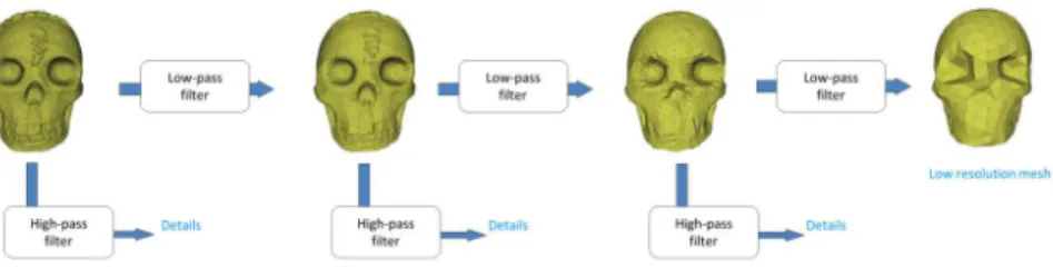
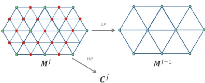
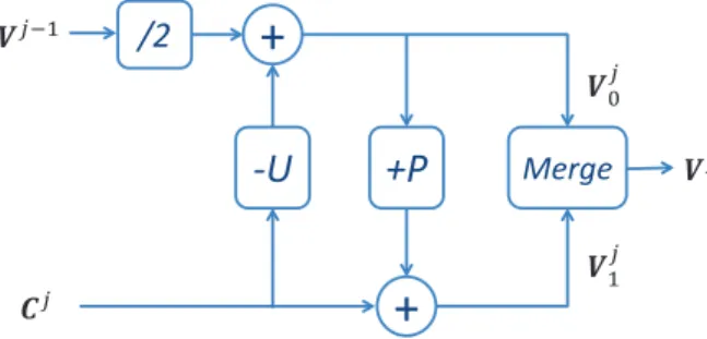
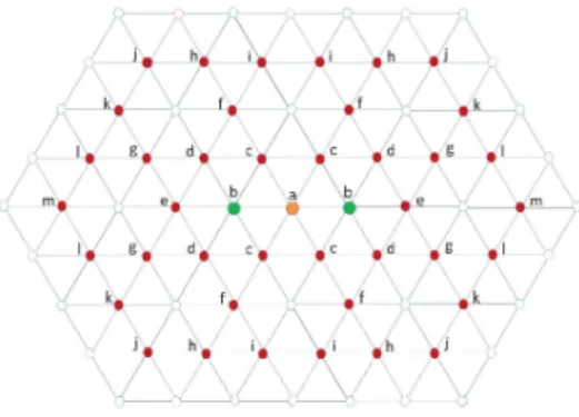
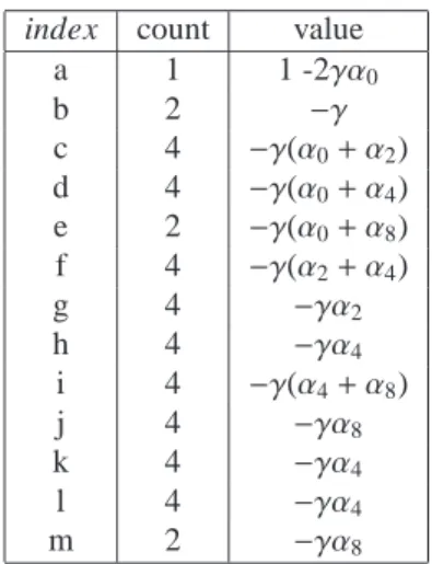
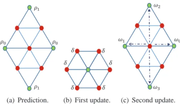
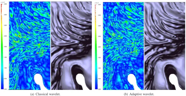
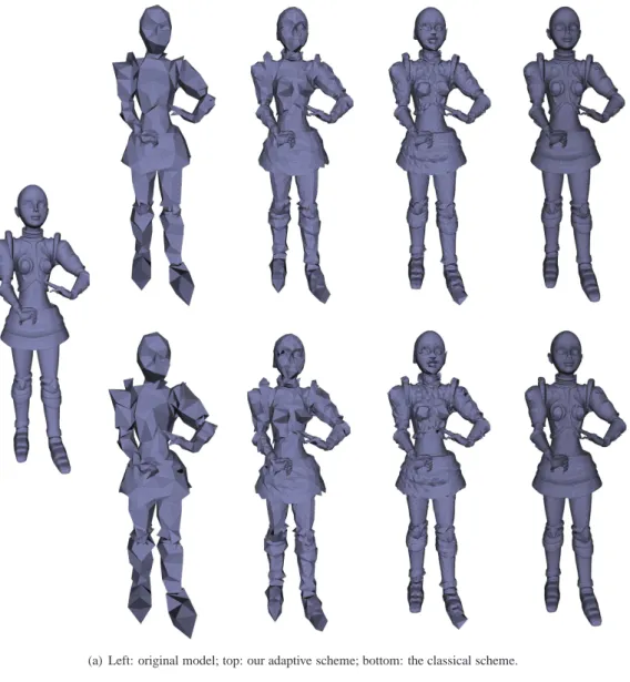
In the wavelet-based SR mesh compression setting, a subdivision scheme is used as a prediction operator during the MRA, to reduce the details lost during this coarsification

The first approach, consists of estimating the channel over all of the three subbands, using the model (3), similar to [5] while the second scheme is a wavelet domain EM

In this chapter, we propose a generalized lifting-based wavelet processor that can perform various forward and inverse Discrete Wavelet Transforms (DWTs) and Discrete Wavelet

Looking at a refocused image after compression, the blur due to compression is unnoticed in out-of focus regions where the quantization blur is mixed to natural geometry blur. As