HAL Id: hal-01685044
https://hal.archives-ouvertes.fr/hal-01685044
Submitted on 16 Jan 2018
HAL is a multi-disciplinary open access archive for the deposit and dissemination of sci-entific research documents, whether they are pub-lished or not. The documents may come from teaching and research institutions in France or abroad, or from public or private research centers.
L’archive ouverte pluridisciplinaire HAL, est destinée au dépôt et à la diffusion de documents scientifiques de niveau recherche, publiés ou non, émanant des établissements d’enseignement et de recherche français ou étrangers, des laboratoires publics ou privés.
Experimental determination of melt interconnectivity
and electrical conductivity in the upper mantle
Mickaël Laumonier, Robert Farla, Daniel J. Frost, Tomoo Katsura, Katharina
Marquardt, Anne-Sophie Bouvier, Lukas P. Baumgartner
To cite this version:
Mickaël Laumonier, Robert Farla, Daniel J. Frost, Tomoo Katsura, Katharina Marquardt, et al.. Experimental determination of melt interconnectivity and electrical conductivity in the upper mantle. Earth and Planetary Science Letters, Elsevier, 2017, 463, pp.286-297. �10.1016/j.epsl.2017.01.037�. �hal-01685044�
Experimental determination of melt interconnectivity and
1electrical conductivity in the upper mantle
2 3Mickael LAUMONIER1*, Robert FARLA1, Dan FROST1, Tomoo KATSURA1, Katharina 4
MARQUARDT1, Anne-Sophie BOUVIER2, Lukas P. BAUMGARTNER2 5 1 Bayerisches Geoinstitut, University of Bayreuth, Bayreuth, Germany 6 2 Institute of Earth Science, University of Lausanne, Geopolis, 1015 Lausanne, Switzerland 7 8 *corresponding author: ML (mickael.laumonier@gmail.com) 9 10 Abstract 11 The presence of a small fraction of basaltic melt is a potential explanation for mantle electrical 12
conductivity anomalies detected near the top of the oceanic asthenosphere. The 13
interpretation of magnetotelluric profiles in terms of the nature and proportion of melt, 14
however, relies on mathematical models that have not been experimentally tested at 15
realistically low melt fractions (< 0.01). In order to address this, we have performed in situ 16
electrical conductivity measurements on partially molten olivine aggregates. The obtained 17
data suggest that the bulk conductivity follows the conventional Archie’s law with the melt 18
fraction exponent of 0.75 and 1.37 at melt fraction greater and smaller than 0.5 vol.% 19 respectively at 1350°C. Our results imply multiple conducting phases in melt-bearing olivine 20 aggregate and a connectedness threshold at ~0.5 vol.% of melt. The model predicts that the 21 conductive oceanic upper asthenosphere contain 0.5 to 1 vol.% of melt, which is consistent 22
with the durable presence of melt at depths over millions years while the oceanic plate 23 spreads apart the mid-ocean ridge. A minimum permeability may allow the rise of Mid-Ocean 24 Ridge Basalts where melt is likely to be present up to 4 vol.% beneath the ridges. 25 26 Keywords (6 max) 27 Electrical conductivity; upper mantle; Low Velocity Zone; melt interconnectivity; olivine 28 aggregate; basalt. 29 30 Highlights 31 • We measured the electrical conductivity (EC) of the melt-bearing olivine aggregate 32 • We note an melt interconnectivity threshold at a melt fraction of 0.5 vol.% 33 • We model EC according to T°C and melt fraction using the conventional Archie’s law 34
• The LVZ & MORB production regions are explained by <1 and < 4% of melt 35 respectively 36 • Low melt fraction (<1%) is consistent with durable presence of melt at the LVZ 37 38 One sentence summary 39
We performed in situ electrical conductivity measurements on partially-molten olivine 40 aggregate to check the mixing law models at low, realistic melt fraction potentially existing in 41 the upper mantle. 42 43
1. Introduction 44
One of the most striking geophysical anomalies identified in the upper mantle is the Low 45
Velocity Zone (LVZ, e.g. Holtzman, 2016) characterized by low seismic velocities and high 46
attenuation and located in the asthenosphere near the Lithosphere-Asthenosphere Boundary 47
(LAB); under oceanic plates, the LVZ appears to coincide in some regions with a 20 to 50 km 48
thick layer that possesses a high electrical conductivity (EC) (up to Log ! = -0.3; ! in S/m) 49
relative to overlying and underlying layers (e.g. Evans et al., 2005; Baba et al., 2006; Naif et al., 50
2013; Sarafian et al., 2015). 51
Several factors that might enhance EC have been invoked to explain these anomalies, such as 52
anisotropy in mineral conductivity (e.g. Poe et al., 2010), water dissolved in nominally 53
anhydrous minerals (e.g. Dai & Karato, 2014), or the presence of melt (e.g. Gaillard et al., 54
2008; Yoshino et al., 2010a; Ni et al., 2010; Sifré et al., 2014). However, conductivity 55
anisotropy in olivine aggregates appears to have an insufficient effect on EC to account for the 56
observed mantle anomaly (Poe et al., 2010; Yang, 2012). In addition, water dissolved in 57
olivine is unlikely to produce the conductivity anomalies observed in the upper mantle 58
(Gardés et al., 2014) because the concentration of water in minerals required to reach upper 59
mantle conductivities (100 to 1000 ppm; e.g. Dai & Karato, 2014) would lead to partial 60
melting of the mantle rocks, accompanied by partitioning of significant proportions of water 61
into a melt phase rather than minerals (Hirschmann, 2006). Anisotropic distribution of the 62
melt may also be a further factor enhancing the EC (Caricchi et al., 2011; Zhang et al., 2014; 63 Pommier et al., 2015a). For these reasons, it seems that the presence of melt is the most likely 64 explanation for the EC anomalies in the upper mantle, supported by melt-solid viscosity and 65 density contrast (Sakamaki et al., 2013). 66 Large differences in transport properties between silicate minerals and melt mean that the EC 67 of silicate melts is orders of magnitude higher than mineral phases (e.g. Tyburczy and Fisler, 68 1995). As a consequence, the bulk EC of partially molten rocks (minerals + melt) varies with 69
the relative fraction of solid and liquid phases, but also with their respective distribution 70
(Glover, 2010 and references therein). A liquid phase should form an interconnected network 71
in a solid aggregate whenever dihedral angles between the two phases are lower than 60°. 72
Since, in olivine aggregates, basaltic melt is distributed as pockets, tubes and films with 73
dihedral angles as low as ~10°, melt is expected to be interconnected and thus contributes to 74
a significant increase of the EC even at melt fractions lower than 1% (Cmíral et al., 1998; 75
Yoshino et al., 2009; Faul & Scott; 2006; Garapić et al., 2013). 76
77
The conductivity of a partially molten assemblage is generally calculated based on a 78
mathematical model with an assumed mineral and melt geometry. The applicability of such 79
models has, to date, not been experimentally investigated, particularly at very low (< 1%) 80
melt fractions, which are likely realistic for the upper mantle. Amongst the numerous mixing 81
laws summarized and described by Glover (2010) and ten Grotenhuis et al. (2005), the 82
conventional and modified Archie’s laws appear very suitable for calculating the EC of upper 83
mantle materials in which both solid and liquid phase contribute to the bulk conductivity 84
according to defined exponents. Other models, such as the tubes, cubes, and sphere+ models 85
(Grant & West, 1965; Waff, 1974) texturally reproduce a melt-bearing aggregate with a melt 86
fraction > 0.05 where pockets (pools) and films wetting grain boundaries are the dominant 87
features of the melt network (Miller et al., 2014). At melt fractions lower than 0.02, the melt 88
principally forms channels residing along grain edges, and can still be interconnected down to 89
very low melt fractions making those models misfit (Garapic et al., 2013; Holtzman, 2016). In 90
spite of the proposed interconnectivity threshold (e.g. Holtzman, 2016), it is expected that the 91
melt raises the bulk conductivity at these low (<0.01%) melt fractions. 92
93
Estimates for the amount of melt potentially present in the upper mantle is still quite 94
uncertain due to a lack of experimental verification of models relating the degree of partial 95
melt to the resulting EC, particularly at very low (<1%) melt fractions. In order to find the 96
most adequate mixing law for mantle rocks containing low melt fractions, we have performed 97
in situ electrical conductivity measurements on olivine aggregate with melt fraction varying 98
from 0 to 100 vol.% at pressures and temperatures up to 3 GPa and 1430°C respectively. 99
From the results, we build a model based on the conventional Archie’s law, which is valid over 100
large range of temperature and melt fraction. Then, we discuss the amount of melt potentially 101
existing in the upper mantle, and its mobility. In addition, we estimate the temperature 102
distribution in the asthenosphere without melt based on the present conductivity 103 measurements of melt-free olivine aggregates. 104 105 2. Experimental procedure 106 2.1. Starting materials and sample preparation 107 Natural olivine from a Lanzarote peridotite (Canary Islands, Spain) and synthetic basalt were 108 employed as solid and liquid starting materials respectively. The Lanzarote olivine consists of 109
a single chemically homogeneous population of Fo92 (Table 1). Optical impurity-free olivine 110 grains were crushed and sieved to obtain a maximum grain size of 100 micrometers. Olivine 111 was used without further treatment (e.g. annealing under special conditions) so as to remain 112 close to natural mantle materials. The basaltic glass was produced by mixing reagent grade 113 oxides and carbonates and fusing the mixture twice in an iron-enriched platinum crucible at 114 1450°C and 1 atmosphere for 3 hours. The resulting homogeneous glass had a composition 115
similar to that of a Mid-Ocean Ridge Basalt (termed “synthesis”, Table 1). Gadolinium was 116 added to the melt (a very incompatible element that concentrates exclusively in the liquid) for 117 neutron tomography observations that are not reported here. The same batch of basalt was 118 used for all experiments. Its liquidus temperature was estimated to be approximately 1270°C 119 at 1.5 GPa from the melting temperature during synthesis and from EC measurements with 120 the sample with 100% of melt. The glass was then cored to provide starting samples of basalt 121
i.e. for 100% melt fraction experiments, while the rest of the glass was crushed into a fine 122
powder (~ 5 micrometers grain size). This powder was mechanically mixed with olivine 123
grains in order to distribute the glass as homogeneously as possible within the olivine 124
aggregate. Each component was accurately weighed (precision of 0.1 micrograms) to achieve 125
the desired melt fraction, assuming very little density variation between room and 126
experimental conditions (Sakamaki et al., 2013). The mixtures are named according to the 127 volume fraction of added basaltic glass (see also section 4.1). The mixtures and the olivine-128 only aggregate were cold-pressed using a hydraulic press and jig to provide samples 3 mm in 129 diameter and 1.0 to 1.4 mm in length. 130 131 2.2. In situ electrical conductivity measurements 132
In every experiment, the sample was placed between two platinum foils (electrodes) in 133
contact with two thermocouples forming the electrical cell (Fig. 1). An MgO sleeve chemically 134
and electrically insulates the sample from the graphite furnace (see Fig. SI1). Crushable and 135
hard alumina pistons were placed either side of the sample, which was positioned within the 136
hot zone at the centre of the assembly. This zone extending over ~1.5 mm, and was 137
determined by two thermocouples that measured the temperature ~0.3 mm away from each 138
edge of the sample. Experiments where a temperature difference larger than 20°C between 139
the 2 thermocouples was measured, were discarded to avoid EC uncertainties due to large 140
temperature gradients. The furnace and inner parts of the assembly were inserted in a 141
zirconia cylinder used as thermal insulator that was inserted in an unfired 12-mm edge length 142
pyrophyllite cube. Because of the graphite furnace, the absence of a welded-shut capsule and 143
the presence of olivine, oxygen fugacity is believed to approximate FMQ (±1.5 Log unit) 144
conditions Confining pressure was applied to the cube by a six-ram press (MAVO press, 145
Bayerisches Geoinstitute) employing second stage anvils with square truncations of 9-mm 146
edge length (Manthilake et al., 2012). 147
148
#Exp SiO2 TiO2 Al2O3 Cr2O3 Gd2O3 FeO MgO NiO MnO CaO Na2O K2O Total*
Olivine (54) 39.78 0.01 0.02 0.04 8.21 51.37 0.38 0.12 0.06 0.01 0.75 0.01 0.02 0.07 0.20 0.64 0.05 0.04 0.02 0.01 nominal 52 15 2 7.5 8.5 10 3 2 100 Synthesis (20) 52.00 0.31 0.01 15.34 0.01 0.19 1.88 6.81 0.23 0.17 8.68 0.17 0.02 0.02 10.20 3.10 1.96 0.13 0.10 0.04 98.71 2.71 M480 - 100% (16) 48.27 0.40 0.01 14.38 0.02 0.35 1.80 6.15 13.58 0.14 0.17 0.96 0.01 0.01 10.43 3.28 2.09 0.32 0.16 0.13 97.75 0.53 M484 - 10% (15) 48.86 0.73 0.03 12.19 0.02 0.82 1.64 9.59 11.34 0.24 0.56 1.62 0.05 0.15 10.98 3.02 2.19 0.55 0.22 0.23 97.98 0.48 M477 - 4% (11) 50.21 1.10 0.04 15.28 0.02 2.62 2.18 7.31 0.16 0.86 8.77 0.93 0.03 0.19 10.67 3.17 2.19 0.39 0.06 0.10 96.69 0.63 M486 - 2% (14) 49.75 0.52 0.07 11.65 0.02 0.79 1.40 9.76 11.14 0.17 0.50 0.83 0.04 0.19 10.82 3.18 2.06 0.65 0.36 0.27 98.48 0.52 M487 - 1% (8) 48.65 2.40 0.11 11.43 0.05 0.76 1.18 9.50 13.45 0.25 0.64 1.23 0.06 0.15 10.79 3.00 1.73 2.59 0.43 0.32 95.90 1.10 M488 - 0.5% (29) 49.90 0.62 0.01 14.15 0.01 0.33 1.76 8.45 0.24 0.38 8.81 0.69 0.03 0.08 12.48 2.67 1.69 0.67 0.17 0.14 97.21 0.91 M501 - 0.5% (4) 52.09 1.10 0.05 13.54 0.02 0.67 1.25 9.57 10.93 0.14 0.28 2.50 0.00 0.00 8.77 2.47 1.34 1.35 0.19 0.12 98.45 0.59 M510 - 0.25% (11) 51.45 1.13 0.05 10.78 0.03 0.70 1.14 7.83 15.20 0.24 1.16 2.22 0.04 0.15 9.31 2.97 1.10 0.69 0.37 0.07 97.42 0.49
Table 1: Chemical compositions and standard deviations (italic grey font) of the starting materials
149 (Olivine & Synthesis, whereby the nominal and the analyzed composition of the latter are reported) and 150 melt compositions after experiments. All analyses were normalized to 100 wt.%, and the total (*) shows 151 the sum of oxides before correction. The number of analyses performed is indicated after the name of 152 each experiment. 153
In situ EC measurements were performed using a Solartron impedance gain phase analyzer 154
connected to the 4 wires of the 2 thermocouples (see details about impedance spectroscopy in 155
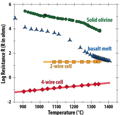
Barsoukov & Macdonalds, 2005, for instance). The very low resistance of the liquid basalt 156
required the use of the 4-wire method for accurate EC measurements, as the internal 157
resistance of a 2-wire measurement is significant (see Fig. SI 2). The graphite furnace was 158
heated manually by controlling the electrical power and acted as a grounded Faraday cage, 159
causing only a minor amount of inductive interference in the frequency range 50 to 250Hz. In 160
a typical run the sample was pressurized for one hour, followed by a heating and cooling 161
cycle, during which impedance spectra were acquired. The 2 thermocouples were switched 162
between the temperature monitor and the impedance spectrometer to avoid interference. 163
After each increase or decrease in temperature the sample was allowed to reach a stable 164
temperature over a period ~1 minute before the sample resistance was measured. Impedance 165
spectra were typically acquired in a frequency range from 1 MHz to 10Hz depending on the 166
signal response of the sample and the temperature (Fig. 2). The temperature was monitored 167
before and after the resistance measurement and was generally found to have remained 168
constant. The measurement was repeated when the temperature was found to have deviated 169
by more than 5°C during the resistance acquisition. Uncertainties on the sample conductivity 170
arise from the sample geometry, temperature measurement and deviation during the 171
measurement and from the determination of the resistance. The total uncertainty calculated 172
by propagating these errors is 0.2 Log units (Laumonier et al., 2015). At the end of the 173
experiment, the furnace power was switched off to quench the sample before slow 174 decompression. 175 176 177
Figure 1: The 12-millimeter assembly employed for in situ electrical conductivity measurements with
178
the MAVO 6ram press. The sample (green) diameter is 3 millimeters before compression. The electrical
179
path (red) includes platinum foil electrodes which sandwich the sample and are in contact with 2 S-type
180
thermocouples connected interchangeably to a temperature monitor and a gain phase impedance
181 analyzer. 182 183 184
Figure 2: Impedance spectra in the Nyquist plane and equivalent electrical circuits (Huebner &
185
Dillenburg, 1995) obtained at low (A: T<1200°C) and high (B: T>1200°C) temperatures on the pure
186
basalt sample. R, C and L in electrical circuits stand for resistance, capacitance and inductance
187
respectively. The real resistance (yellow R) is shown by a yellow symbol.
188
Electrical conductivity mechanisms for minerals and melts have been extensively described in 189
the literature (e.g. Roberts & Tyburczy, 1999; Gaillard, 2004; Yoshino et al., 2010b; Yoshino & 190
Katsura, 2013; Laumonier et al., 2015). It is worth to recall, however, the temperature 191
dependence of the electrical conductivity ! (S/m) according to the Arrhenius Law: 192
! = !! !"#!(!!!!∆! ℜ!) (Eq. 1)
where !0, Ea, P, ∆! and ℜ are a pre-exponential term (S/m), the activation energy (J/mol), the 194 pressure (bar), the activation volume (cm3/mol) and the gas constant (J/mol/K) respectively. 195 196 2.3. Post-experiment analysis 197
Once recovered, the assembly was cut in the middle along an axial plane of the sample, 198
mounted in epoxy resin and polished for textural and chemical analyses. The distribution of 199
the melt and the sample dimensions were characterized by Scanning Electron Microscopy 200
(SEM) with a typical acceleration voltage of 20 to 22 kV. Crystal size distribution and 201 orientation were measured by Electron Backscatter Diffraction on a ZEISS SEM, Leo Gemini 202 1530 with a Schottky field emission gun employing an accelerating voltage of 20 keV and a 203 beam current of about 2.0 -2.5 nA using a 60 mm aperture (more details about the methods in 204 Supplementary Information). 205 Chemical compositions of melt and minerals (olivine) were quantified by an Electron Probe 206 Micro Analyzer with unfocused (10 micrometers) and focused (1 micron) beams respectively, 207 with an acceleration voltage of 15 kV and beam current of 150 nA. The water content was 208
measured using the Cameca IMS 1280HR at the Swiss SIMS laboratory of the University of 209
Lausanne (Switzerland) under a 10kV Cs+ primary beam with a ~1.5 nA current, resulting in a 210
typical spot size of ~10 µm. To minimize the water background in the machine, samples were 211
mounted in indium with a reference material. Before each measurement, the surface was 212
cleaned using a 25µ rastered presputtering beam, for 240 seconds (more details about the 213 methods in Supplementary Information). 214 215 3. Results 216 Table 2 shows the experimental conditions and fitting parameters for the eleven experiments 217 conducted with in situ EC measurements. One run was performed at a constant temperature 218
(M523) while all others followed similar heating and cooling cycles. All experiments were 219
carried out at a pressure of 1.5 GPa, except M501 that was conducted at 3 GPa in order to 220
investigate the effect of pressure on EC. The explored melt fraction, based on the initial 221
fraction of added basaltic glass, ranges from 0 (olivine-only) to 100 vol.% (basaltic melt only). 222
223
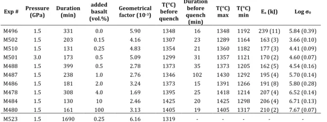
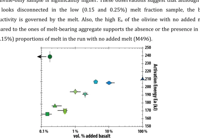
Exp # Pressure (GPa) Duration (min) added basalt (vol.%) Geometrical factor (10-3) T(°C) before quench Duration before quench (min) T(°C)
max T(°C) min Ea (kJ) Log σ0 M496 1.5 331 0.0 5.90 1348 16 1348 1192 239 (11) 5.84 (0.39) M502 1.5 203 0.15 4.16 1307 23 1289 1164 163 (3) 3.66 (0.10) M510 1.5 131 0.25 4.83 1354 21 1360 1182 177 (3) 4.41 (0.09) M501 3.0 173 0.5 5.09 1299 31 1357 1121 170 (2) 4.60 (0.07) M488 1.5 399 0.5 2.78 1373 35 1373 1205 162 (5) 4.54 (0.16) M487 1.5 238 1.0 2.76 1346 102 1430 1292 195 (4) 5.70 (0.14) M486 1.5 181 2.0 3.24 1373 15 1391 1266 191 (8) 5.80 (0.28) M478 1.5 308 4.0 1.69 1395 25 1418 1214 207 (4) 6.52 (0.14) M484 1.5 130 10 2.46 1425 20 1425 1298 206 (4) 6.71 (0.13) M480 1.5 161 100 3.13 1405 19 1405 1317 210 (2) 7.67 (0.07) M523 1.5 1690 0.25 6.16 1319 - - - - -
Table 2: Experimental conditions for EC measurements and fitted activation energy Ea and 224 preexponential factor !0 (S/m), with standard deviations into brackets. T°C max to T°C min defines the 225 temperature interval for the fitting of Ea and !0. 226 227 3.1. Electrical conductivity of melt-bearing olivine aggregates 228
The EC of the olivine-only sample (M496) for several heating-cooling cycles is shown in 229
Figure 3. During the first heating, the EC increased with temperature, corresponding to a low 230
activation energy (Ea ~ 50 kJ/mol), likely due to the presence of moisture up to ~700°C. 231
Between ~800 and ~1230°C, Ea is a factor of two higher than at lower temperatures (Ea ~ 100 232
kJ/mol) due to hopping (also called small polaron) conduction and potential grain boundary 233
effects (Wannamaker & Duba, 1993; Sakamoto et al., 2002; Yoshino et al., 2009). At 234
temperatures above 1230°C, high Ea (239 ±11 kJ/mol) indicates that ionic conduction (e.g. 235
Yoshino et al., 2009) is the dominant mechanism, although there may still be minor 236 contributions from other mechanisms (see also Gardés et al., 2014). 237 The conductivity of sample M510 that contained 0.25 vol.% of added basalt is similar to that 238 of pure olivine below the basalt liquidus temperature (1270°C), but it becomes significantly 239
higher than olivine at temperatures above 1300°C (Fig. 3). However, during the following 240
cooling and heating cycles, the conductivity remains higher than that for pure olivine, 241
probably due to the better wetting properties of melt once it has overshot the liquidus 242
temperature and distributed through the solid matrix. The effect of crossing the solidus 243 temperature of the basalt is not visible in the experiment involving 0.25 vol.% of added basalt, 244 probably due to the low amount and initial distribution of melt (Fig. 3). 245 In the case of the sample composed of basaltic melt only (M480), the jump observed around 246
880°C during the first heating can be explained by improved contact between sample and 247
electrodes upon relaxation of the glass once the glass transition temperature has been 248
crossed. Around 1090°C (grey arrow on Fig. 3), the slope suddenly increases from 74 ±9 to 249
248 ±10 kJ, probably coinciding with the solidus temperature of the basalt. The value of 248 250
kJ has no physical meaning because the basaltic glass may have partly crystallized, and the 251
formed crystals may have gradually melted at these temperatures. The very good 252
reproducibility of the conductivity measurements during the different heating and cooling 253
cycles attests to the accuracy of the measurements and the limited loss of melt from the 254 sample chamber (see also section 4.1). 255 256 257 Figure 3: Reciprocal temperature versus electrical conductivity of samples containing 0, 0.25 and 100% 258
of basaltic melt at 1.5 GPa. The activation energy (Ea) is indicated for the pure olivine sample, with
259
probable conduction mechanisms. Black and grey arrows correspond to feature most likely caused by
260 the glass transition and the solidus of the basalt respectively. The conductivity values obtained during 261 cooling are superimposed by the last heating path. The error in temperature is smaller than the symbols 262 while the maximum error in EC is 0.2 log unit. 263
264
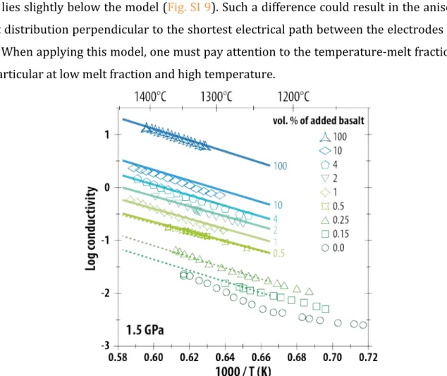
The logarithmic EC of the pure olivine aggregate and of olivine aggregates containing various 265
fractions of basaltic melt are displayed as a function of reciprocal temperature in Fig. 4. For all 266
melt fractions investigated, the EC increases with the temperature but is clearly very sensitive 267
to the fraction of melt: the higher the melt fraction, the higher the conductivity. For instance, 268
at 1300°C, the addition of 0.5 vol.% of basaltic melt increases the EC by one order of 269
magnitude compared to the pure olivine aggregate; the addition of 10 vol.% of melt increases 270
the EC by 1.8 log unit, and the pure basalt liquid end-member is by 2.6 orders of magnitude 271
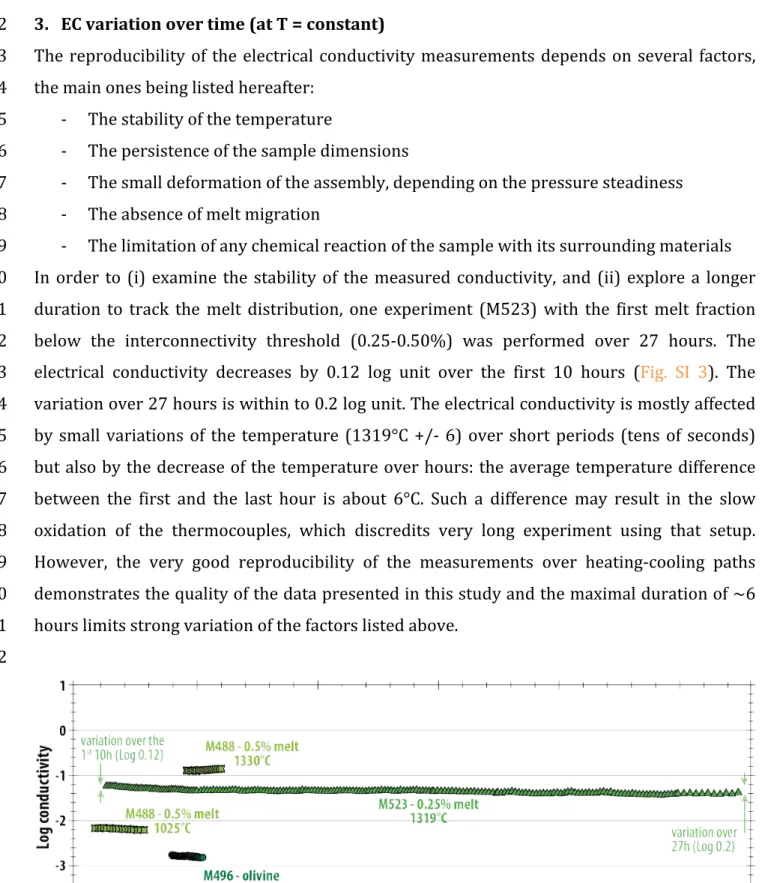
more conductive. These relations are not affected by run duration: experiment M523 was 272
performed at a single temperature of 1319°C for 27 hours, but the conductivity is consistent 273
with data from M510 which contained the same melt fraction but followed a temperature-274
time cycle similar to the other experiments (Fig. 4; see also Fig SI 3). M488 and M501 both 275
contained a basalt melt fraction of 0.5 vol.% and were conducted at 1.5 and 3.0 GPa 276 respectively have identical conductivities within the error. 277 278 Figure 4: Reciprocal temperature versus EC of basaltic melt and olivine aggregate with 0 to 10 vol.% of 279 added basaltic melt at 1.5 GPa (symbols). An olivine aggregate experiment containing 0.5 vol.% of added 280 basalt was also conducted at 3 GPa (empty diamonds). The range of conductivity measured at constant 281 temperature in experiment M523 is shown by the empty triangles. Lines correspond to the fit of the data 282
using equation (1) and fitting parameters are presented in Table 2.
283 284
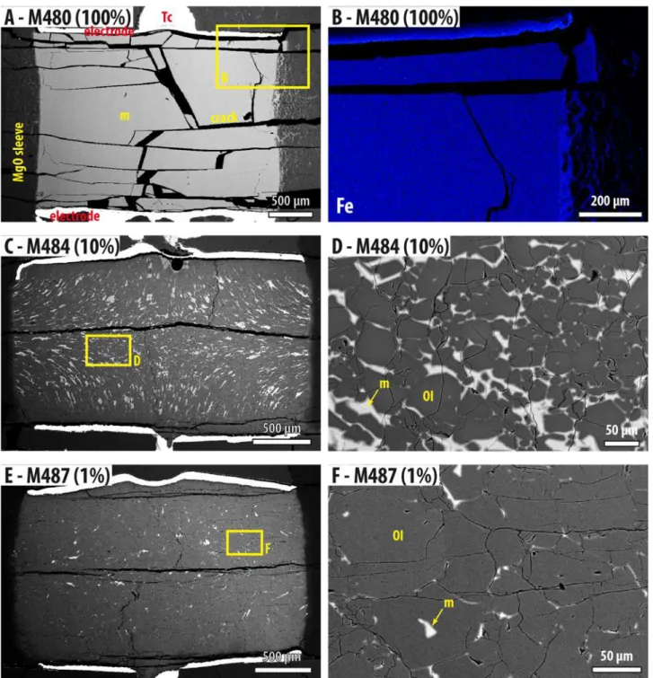
3.2. Textural results 285
SEM observations of the recovered experimental charges showed that the initial cylindrical 286
shape of the sample was preserved through the experiment with only minor irregularities, 287
mainly where the electrodes are in contact with the thermocouples (Fig. 5; Fig. SI 4). The 288
horizontal cracks observed throughout the sample may have been caused by tensile stresses 289
during decompression and were omitted from the calculation of the geometrical factor 290
(corresponding to aspect ratio of the sample, i.e. the surface divided by the length; Table 2). 291
The grain size ranges up to 100 microns, but shows no significant grain growth over the 292
duration of the experiments (Fig. SI 5). The effect of grain size on EC was not investigated 293 here. Low magnification images show a relatively homogeneous distribution of melt, which is 294 visible as pockets ~50 microns across in the experiment where ≤ 2 vol.% of melt was added 295 (Fig. 5A, C & F). The elongated melt pockets appear to follow the flow lines typically induced 296
by compressive deformation, i.e. sub-normal to the electrodes at the top and bottom of the 297
sample, rotating sub-parallel to the electrodes in the centre of the sample, suggesting a small 298
deviatoric stress was present during the experiments (Fig. 5A and Fig. SI 4C; see more in 299
Section 4.1). At higher magnification, we note the presence of melt as films and tubes, 300
displayed as lines and dots respectively in 2D sections (examples of the labels on Fig. 5B). The 301
melt appears to be fully interconnected for basalt melt fractions ≥ 2 vol.% but not 302
interconnected at fractions < 0.5% (Fig. 5 D & G). A comparison in the distribution of calcium 303
between experiments with 0.5 and 0.25 vol.% melt contents reveals the presence of small 304 melt-associated Ca-rich pockets in both samples but Ca-rich films are not visible in the sample 305 with 0.25 vol.% of added melt (Fig. 5 E & H). 306 307 3.3. Chemical composition and water content of experimental products 308
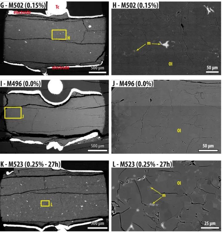
The chemical composition of olivine after experiments is almost identical to the starting 309
composition (Fig. SI 6). The slight increase of the Fo content, by up to ~0.01 (molar Mg/(Fe + 310
Mg) ), is probably related to minor reaction with the MgO capsule (see section 1 of 311 supplementary materials), slight loss of Fe to the Pt electrodes and/or a minor readjustment 312 in mineral/melt Fe-Mg partitioning. 313 The chemical composition of the melt in the experimental products is similar to that of the 314
starting basaltic melt (Table 1). There is some variation apparent in the concentrations of 315
MgO, Al2O3, and FeO and a small variation in the sodium concentration (electrical charge 316
carriers) but none of these differences exceed 10%, except for the experiments with a basalt 317
fraction of 0.5 vol.% that show changes that are slightly larger than this. The chemical 318
compositions and textural observations give no indication that interactions occurred between 319
olivine crystals and melt that could have significantly affected the EC measurements. 320
The water content measured in olivine is below the detection threshold, thus implying a 321
concentration of water lower than 10ppm in the solid material, in comparison with the dry 322
forsterite used as a calibration standard. In contrast, the glasses contain substantial amounts 323
of water, with the experiments containing the lower melt fractions producing the most 324
hydrous glasses (Fig. 6). The experiment with no crystals produced a glass with little water 325
(0.1 wt.% H2O), slightly more than the starting glass (0.03 wt.%). Experiments with lower 326
melt fractions resulted in glasses containing between 0.54 wt.% H2O (10 vol.% of added 327
basalt) and 0.74 wt.% H2O (2 vol.% of added basalt) (Fig. 6). The glasses from the experiments 328
with 0.25, 0.5 and 2 vol.% added melt have similar water contents but there is no clear a 329
correlation between the water content in the experimental glasses and the added melt 330
fraction (Fig. 6). 331
332
333
Figure 5: Back-Scattered Electron (BSE) images (A to D, F and G) and relative concentration maps for
334
calcium (E and H) in experiments involving 2, 0.5, and 0.25 vol.% of added basalt. On SEM images, the
335
metal electrodes are white, the melt (m) is light grey and olivine (Ol) is dark grey. Calcium mapping
336
highlights melt pockets and films around olivine crystals (black and dark blue areas). Rare
337
orthopyroxene crystals (Opx) are present at the top of the sample in image H, coming from impurity in
338
the starting material.
340
341
Figure 6: Water contents (bold font) of melts in experimental products reported with the number of
342 analyses (number in brackets). The average water content in melts from experiments with added melt 343 fractions between 0.25 and 0.10 is 0.68 ±0.09 wt. % (horizontal green line). 344 345 4. Discussion 346 4.1. Experimental limitations 347 4.1.1. Chemical contamination 348 The experiments were conducted for durations as short as possible (except M523) in order to 349 limit melt loss or chemical contamination of the sample with the surrounding host assembly. 350
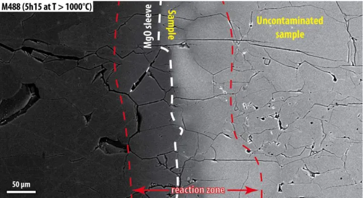
Only the experiment conducted with pure basaltic liquid (M480) shows a minor amount of 351
melt percolating into the MgO sleeve (Fig. SI 4 A & B). Based on the presence of melt after 27 352
hours at 1319°C, including regions close to the MgO sleeve, we believe that there is no 353 significant escape of liquid from the sample over the experimental duration. A stable sample 354 volume and EC measurement is, therefore, maintained over the duration of the experiments. 355 The contamination of the sample by the MgO sleeve is limited to a narrow peripheral layer of 356 100 to 150 micrometers in the longest duration experiment (excluding M523), representing 357 less than 5% of the sample diameter. On the other hand, the platinum electrodes alloy to some 358 degree with iron from olivine and the melt, the latter remaining homogeneous in composition 359
(see iron distribution in the 100% melt experiment, Fig. SI 4B) except in a narrow (< 50 360 microns) layer at the contact with electrodes. This alloying, however, does not influence the 361 electrical conductivity of the sample. 362 4.1.2. Textural equilibrium 363
Once above the basalt liquidus temperature of the first heating, the EC reaches a value 364
reproduced during later cooling and heating cycles (see the experiment with 0.25 vol.% of 365
basalt, Fig. 3). According to this observation, we conclude that the melt should have promptly 366
percolated through the sample and wetted the electrodes. The examination of the experiment 367
M523 shows that melt pockets are preserved even after 27 hours without further wetting of 368
the crystal aggregate (Fig. SI 4K & L). Coaxial strain in the experiments would have favored 369
the percolation of the melt through the aggregate as highlighted by preferentially oriented 370
melt pockets in samples involving 2 and 10 vol.% of added basalt. The melt distribution 371
geometry in the samples is complex and it is not clear how small amount of coaxial strain 372
would have contributed to enhance the EC in the samples. However, the consistent 373
orientation of these persistent melt pockets parallel to the electrodes (perpendicular to the 374
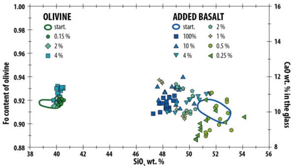
electrical path) should have not led to an increase in the bulk conductivity of the sample 375 (Zhang et al., 2014). 376 4.1.3. Melt fraction determination 377 The determination of post-experimental melt fractions by SEM observation is challenging due 378 to the image resolution, and the conversion from 2D to 3D. Post-experimental melt fraction 379 estimates are usually under-estimated at low magnification due to the difficulty in observing 380
the thin melt films and pockets, particularly for the samples with the lowest melt fractions 381 (Fig. SI 7). On the other hand, at higher magnification, heterogeneity in melt distribution, i.e. 382 the presence of scattered melt pockets of different sizes, leads to biased estimates of the melt-383 crystal ratio. This can lead to errors in the melt fraction determination that are larger than the 384 initial mass ratio of the mixed components. Consequently, though the glass fraction observed 385 on post-mortem SEM picture is similar to the one determined from the initial weight ratio of 386 olivine and basalt in the starting material of each experiment, we rely only on the latter (Fig. 387
5, Fig. SI 4 and Fig. SI 7). In addition, it is possible that the pure olivine aggregate does not 388
remain melt-free at high temperatures (for instance, T > 1350°C), since the solidus 389
temperature of an olivine aggregate particularly in the presence of even minor amounts of 390
H2O could easily be over stepped (Hashim, 2016). However, according to Chantel et al. (2016), 391
the very low amounts of melt that could be expected in the pure olivine aggregate (< 0.1%) 392
would not wet the grain boundaries, as reflected in the very high EC compared to samples 393
with a low added basalt fraction (Table 2 and Fig. SI 7) even though intergranular mass 394
transport is strongly influenced by minor amounts of hydroxyl as proven by the work of 395 Gardés et al. (2012). It is shown that activation energy of diffusion in hydrous-saturated grain 396 boundaries is reduced compared to dry grain boundaries. 397 398 4.2. Implications of the melt distribution 399 For experimental durations investigated in this study (<27 hours), melt pockets are preserved 400
regardless of the melt fraction (Fig. 5), including when the melt is not fully interconnected 401
(melt fraction < 0.5 vol.%). Complete redistribution of a small melt fraction appears to require 402
much longer timescales than employed in the experiments. Similar persistent melt pockets 403
were also observed by Garapic et al. (2013) after 430 hours at high temperature. 404
Alternatively, a threshold melt fraction may be required for the complete redistribution of 405
melt pockets, as discussed in the next section. Their stability excludes any textural evolution 406
that would affect the electrical results. 407
Although tubes are common features in all samples, films on the grain boundaries are not 408
recognized in the samples containing 0.25 vol.% of added basalt or less (Fig. 5). Such feature 409
seems determinant to switch from a low degree of interconnectivity where films are not 410
present to a high degree of interconnectivity where films are present alongside pockets and 411
tubes. The presence of films implies dihedral angles smaller than 10° (Cmíral et al., 1998). Our 412
observations therefore suggest that olivine does not exhibit dihedral angles less than 10° in 413
the presence of very small melt fractions. Furthermore, dihedral angles were observed to be 414
temperature-dependent in melt-bearing olivine aggregates ranging from 19° to 9° between 415
1300°C and 1450°C (Yoshino et al., 2009). In the olivine-basalt system, the disappearance of 416 films with lower melt fraction seems to record the interconnectivity threshold as supported 417 by the EC measurements (see next section). However, our experimental setup does not allow 418 us to distinguish between the individual effects of pockets or films on the bulk conductivity of 419 the partially molten assemblages. 420 421 4.3. Choice of the mixing law 422 The activation energy and pre-exponential factor were determined for each experiment based 423
on an Arrhenius relationship of EC (Eq. 1; Table 2; Fig.4). The calculated EC values closely 424
reproduce the experimental data (Fig. 4). For the pure olivine aggregate, only data points 425
obtained at temperatures higher than 1230°C were used to determine the fit, corresponding 426
to temperature where ionic conduction is assumed to be the dominant transport mechanism 427
(Fig. 3 and Section 6 of supplementary materials). The value of the EC fitted at 1350°C is 428
plotted against the added melt fraction in Figure 7: from 100 down to 0.5 vol.%, the EC of 429
partially-molten olivine aggregates defines a trend significantly higher than the models 430
commonly used in the literature, such as +Spheres, Tubes, and Cubes models (Grant & West, 431
1965; Waff, 1974) (Fig. 7), which can be modeled most closely using the Conventional Archie’s 432
law (Eq. 2): 433
!!"#$ = !! !!! (Eq. 2)
434
where !!"#$ is the EC of the system, !! the melt fraction in vol.%, !! the EC of the liquid and m 435
is a measure of how the ratio !!"#$
!! varies as a function of melt fraction and degree of
436
interconnection of the melt (Glover, 2010 and references therein). The value m will be < 2 for 437
a well-interconnected liquid phase and it will tend to unity only if the liquid phase is fully 438
interconnected and is the only conductive phase (Glover, 2010). In our case, at 1350°C and 439 added basalt fraction > 0.5 vol.% (high degree of interconnectivity), the power law exponent 440 m = 0.75 ±0.02 while the first term is the conductivity of the basaltic liquid, i.e. log !! = 0.89 441 ±0.03 (! in S/m). This low value of m indicates that the liquid phase is highly interconnected 442 and that another conduction mechanism contributes to the bulk conductivity so as to provide 443 a value of the exponent m < 1. The existence of another conduction mechanism than the melt 444 is also demonstrated by the higher EC than given by the parallel model (“PM” in Fig. 7), which 445
is supposed to represent the maximum EC where the melt is the unique conduction 446 mechanism. 447 448 449 Figure 7: Electrical conductivity versus the fraction of added basalt (in volume %) (Log scale) from the 450 current experimental data (blue to green symbols which are identical to legend of Fig. 4) compared with 451
the Modified Archie’s law (MA), Conventional Archie’s law (CA), Parallel model (PM), +Spheres (+S),
452 Cubes (C), Tubes (T) and -Spheres (-S) models (curves) from the literature at 1350°C. See text for model 453 references. Black segments represent the error on the model fraction estimated by image analysis (see 454 supplementary information). 455 456 The maximum value of m (0.84 ±0.05) is obtained when considering the experiments with 0.5 457 to 2 vol.% of added basalt that contain similar water contents (~0.68 ±0.09 wt.%). Based on 458
the experiments of Ni et al. (2011) at 1450°C, the effect of 1.1 wt.% of water would increase 459
the EC by 0.3 log unit only (Log σ = 1.0), and the resulting m exponent would be 0.86 ± . 460
Therefore, the value of the exponent m cannot be the result of the small water content 461
difference observed in the experiments. Since the melt composition does not vary 462
significantly, in particular in the Na content, the reason why the value of m is lower than unity 463
may reside in the solid phase, even though the EC of the latter is almost 3 log units lower than 464
the basalt melt. Grain boundary effects and/or the existence of an electric double layer 465
(Grahame, 1947) might enhance EC and would argue in favor of a low m exponent after the 466
Na-coating of crystallizing olivine but these concepts cannot be demonstrated by our 467
experiments. 468
The m value we find is comparable to that (0.89) experimentally determined by Yoshino et al. 469
(2010a), but significantly different from that calculated by Miller et al. (2015) of 1.3 ±0.3. Such 470
a value is inconsistent for melt fractions lower than 0.8% since the conductivity of the melt-471
bearing olivine aggregate becomes lower than that of olivine-only (Log σ = -2.05; Constable, 472
2006). The exponent calculated by Yoshino et al. (2010a) on an olivine-carbonatite system (m 473
= 1.14) implies a very good interconnectedness, but the existence of one conducting phase 474 only, probably due to the higher conductivity of carbonatite melt than basaltic one (more than 475 one order of magnitude). 476 477 4.4. Interconnectivity threshold of the melt fraction (0.5 vol.%) 478 For experiments with added basalt fractions of 0.25 and 0.15 vol.%, the EC is lower than the 479
trend previously described (dashed line, Fig. 7) but still higher than the olivine-only aggregate 480
defining a higher exponent of m = 1.37. We deduce that the basaltic melt is no longer fully 481
interconnected but remains still well-interconnected overall, and still contributes to an 482
increase in the bulk EC. Therefore, under our experimental conditions, an interconnectivity 483
threshold exists at a added basalt fraction of 0.5 vol.% in the olivine aggregates. No 484 mathematical law reproduces such a change in connectedness with the melt fraction. Such a 485 threshold is likely linked to the appearance/disappearance of films, switching to a low/high 486 degree of interconnectivity and resulting in different electrical transport properties. The low 487 degree of interconnectivity is explained by the persistence of tubes in the solid aggregate. The 488 threshold evidenced here occurs at very low melt fraction, and could be easily masked by the 489 high jump in EC observed upon melting observed in other study (e.g. Maumus et al., 2005). 490
The threshold depends on the melt distribution (tubes / films…), thus on the wetting 491
properties of the melt with the solid phase (Yoshino et al. 2009; Zhu et al. 2011). 492
493
4.5. Model of the EC of partially-molten olivine aggregate 494
Since the difference between the conventional and the modified Archie’s laws is negligible 495
above the interconnectivity threshold (added basalt fraction ~0.5 vol.%), we use the 496
conventional law to fit all data from this study with a high degree of interconnectivity: we 497
now incorporate the temperature dependence on the EC to the previous fit by regressing the 498
evolution of the Archie’s law parameters with temperature. The correlation of the two 499
parameters with temperature provides the following simplified equation: 500
!"# ! = !" + ! ∗ !"# !!+ (!" + !) (Eq. 3) 501
where !, T, !! are the electrical conductivity (in S/m), the temperature (in Kelvin) and the
502 melt fraction respectively, and a to d are fitting parameters determined from the experiments 503 (a = 3.66E-04 ±8E-6; b = 0.151 ±0.013; c = 4.52E-03 ±1E-4; d = -6.448 ±0.16). The mixing model 504 integrating both temperature and melt fraction is valid for temperatures higher than 1230°C 505 and melt fractions !! higher than 0.5 vol.%. 506
The same Equation 3 can be applied to fit calculate the EC of partially molten olivine 507
aggregate with melt fraction ranging between 0.5 down to 0.15 vol.% and temperature higher 508
than 1230°C. In that case, the fitting parameters are a’ = 1.57E-04 ±4E-6; b’ = 1.113 ±0.006; c’ = 509
3.92E-03 ±9E-5; d’ = -4.082 ±0.14. In this range of melt fraction with a lower degree of 510
connectivity, if m = 1.37, then the preexponential factor A = 2.9 log units, being a value too 511
high for the conductivity of basaltic melt. Hence, there must be other phase more conductive 512
than olivine to get m = 1.37, such as, for instance, grain boundary effects that become more 513 and more significant at lower melt fractions (Marquardt et al., 2015). 514 515
Both models reproduce very closely the experimental results (see Fig. SI 8) and is compared 516
with data from the literature (Fig. 8) except the solid end-member for which the Arrhenius fit 517
is used (Eq. 1; Table 2). 518
Conductivities for both solid and liquid end-members fall in the range of their respective 519
values defined by previous studies, though most of the melt measurements were performed 520
on basaltic liquids that do not appear to respect an Arrhenius law (Fig. 8) (Presnall, 1972; 521
Waff & Weill, 1975; Tyburczy & Waff, 1983; Pommier et al., 2010; Ni et al., 2011). The EC 522
measurements on the pure olivine aggregate reproduce closely those reported for olivine by 523
Poe et al. (2010) along the (100) and (001) axis orientations at lower temperatures (T < 524
1250°C) but the data diverge quite significantly at higher temperatures. A comparison 525
between our measurements and those reported for dry olivine and olivine containing 50 ppm 526
of H2O (Jones et al., 2012) is consistent with SIMS analyses indicating < 10 ppm H2O in our 527 olivine aggregates. Caution should be taken, however, when comparing transport mechanisms 528 determined for single crystals, with those of polycrystalline aggregates since models for this 529 conversion have not be thoroughly tested. Finally, the extrapolation of olivine EC measured at 530
low temperature (typically <1200°C) to natural upper mantle conditions by assuming a 531
constant Ea may be misleading, in particular at low melt fractions and high temperatures 532 where the contribution of olivine to EC is significant. 533 534 Figure 8: Electrical conductivity plotted against the reciprocal temperature for basalt, olivine aggregate 535
and partially molten olivine aggregates with various fractions of basalt. Thick curves are model
end-536
member conductivities (basalt and olivine aggregate), plotted with the experimental data (3 point stars
537
and circles respectively). Modeled mixtures from this study (purple to pink) are also shown. Previous
538
studies on basalt with comparable compositions are shown as thin blue curves (Presnall, 1972; Waff &
539
Weill, 1975; Tyburczy & Waff, 1983; Pommier et al., 2010; Ni et al., 2011), whereas previous olivine
540
measurements are shown by thin green curves (Sakamoto et al., 2002; Constable, 2006; Poe et al., 2010;
541
Jones et al., 2012) and partially molten olivine aggregate measurements (Yoshino et al., 2010; Caricchi et
542
al., 2011; Zhang et al., 2014). The two values from Zhang et al (2014) correspond to measurement in the
543
direction normal (lower value) and parallel (higher value of conductivity) to the shear direction. Melt
544
proportions from Yoshino et al. (2010a) and Caricchi et al. (2011) are expressed in weight %.
545 546
The comparison of the EC of partially molten olivine aggregate with the study of Yoshino et al. 547
(2010a) (10, 3 and 2 wt.% of basalt added to olivine aggregate), corresponding to volume 548
proportions of 8, 2.4 and 1.6 vol.% when assuming densities of 3.3 for olivine and 2.7 for the 549
basalt), show similar values at T < 1300°C, but the higher Ea they found and the presumed 550
absence of water in their experimental products results in lower EC at higher temperatures 551
(Fig. 8). One significant difference between the two studies is the starting grain size (up to 100 552
micrometers here against a few micrometers in Yoshino et al., 2010a). Our model also gives a 553
higher conductivity than deformed partially-molten olivine aggregates (Caricchi et al., 2011; 554
Zhang et al., 2014). In the study of Zhang et al. (2014), the electrical anisotropy of a peridotite 555
with 2 vol.% of basaltic melt is investigated during deformation. The EC in the direction 556
parallel to the shear direction is one order higher than in the one normal to the shear plane. 557
Such a difference comes from the good melt interconnection and agrees with our results (Fig.
558
8). In addition, the EC value of the experiment with 2 vol.% of added melt lowered by one 559 order of magnitude would provide a melt fraction close to 0.25 vol.%, therefore in the field of 560 low degree of interconnectivity, such as suggested by Zhang et al. (2014). 561 562 4.6. Estimation of the melt fraction in the upper mantle 563 4.6.1. Oceanic asthenosphere 564 Our model for the EC of melt-bearing olivine aggregates can be adapted for the interpretation 565 of melt-induced electrical anomalies located in the upper mantle, in situations where (i) the 566
melt is likely basaltic in composition and exceeds 0.15 vol.%, (ii) assuming the EC of 567
peridotite is similar to that of an olivine aggregate, (iii) the grain size has negligible effect on 568
the EC and (iv) regions are deformed by long-range tectonic stresses. The absence of a 569 measureable pressure effect on the EC between 1.5 and 3.0 GPa implies that the mixing model 570 developed in this study can be applied to understand the conductivity structures of the LAB 571 and LVZ. Our model implies an interpreted maximum melt fraction of 0.4 - 1 vol.% to explain 572 the conductive, off-axis region of the East Pacific Rise (off EPR), assuming a temperature of 573
1350°C (Evans et al., 2005; Baba et al., 2006; Sarafian et al., 2015) (Fig. 9A). The lower EC of 574
the Cocos plate LAB (log σ = -0.6 to -0.9 S/m) and higher assumed temperature (1420°C; Naif 575
et al., 2013) leads to a melt fraction range of 0.3 to 0.5 vol.%, implying that the melt would not 576
be fully interconnected (Fig. 9A). These melt proportions estimated for the top of the 577
asthenosphere in these two regions are lower than previous estimates (e.g. Evans et al., 1999, 578
2005; Baba et al., 2006; Hirschmann, 2010; Yoshino et al., 2010a; Ni et al., 2011; Naif et al., 579
2013) as a result of the mathematical models previously employed underestimating bulk EC 580
at low melt fractions. On the other hand, the melt fractions remotely estimated using our 581
model agree with estimates of <1% based on melt migration and incremental melting models, 582
in which there is a maximum melt fraction that can be retained by the solid matrix (Kelemen 583
et al., 1997). They also agree to the value of 0.5 vol.% estimated by Chantel et al (2016) based 584 on ultrasound velocity measurements. 585 586 4.6.2. East-Pacific Rise and Mid-Ocean Ridge regions 587 The melt fraction estimated beneath the EPR crest will depend strongly on the solidus of the 588
peridotite and, therefore, on the adiabatic gradient. We use a melting depth interval of 589
between 60 and 100 km (Langmuir et al., 1993; Baba et al., 2006; Key et al., 2013) and employ 590
the volatile-poor peridotite solidus determined by Hirschmann (2000) (Fig. 9B) to constrain 591
the pressure (2 to 3 GPa) and temperature (1330 to 1400°C) of the melting zone beneath the 592
EPR. Under such conditions, based on the conductivity value of Baba et al. (2006) and our 593
results, we estimate melt proportions of between 0.8 and 4 vol.%, which is consistent with the 594
value of Kelemen et al. (1997, and references therein), although less than half the value of 595
10% proposed by Key et al. (2013). 596
Contrary to the suggestion of Miller et al. (2015), high concentrations of volatiles in the melt 597
(> 0.7 wt%) and olivine aggregate are not required to explain conductive anomalies in the 598
oceanic upper mantle, under ridge or at the top of the asthenosphere. However, higher 599
concentrations of volatiles dissolved in the melt would significantly increase the bulk 600
conductivity (Gaillard 2004; Ni et al., 2011; Sifré et al., 2014; Laumonier et al., 2015) and the 601 temperature, melt fraction and volatile concentration would be highly correlated. It therefore 602 becomes impossible to resolve between the effects of temperature or volatile concentration 603 using EC alone and some additional constraint needs to be found, a problem that is beyond 604 the scope of this study. 605 606 Figure 9: (A) Reported values of electrical conductivity of various upper mantle anomalies: East Pacific 607
Ridge (EPR, Baba et al., 2006), Off axis EPR (Off EPR, Evans et al., 2005; Baba et al., 2006), Cocos plate
608
(Naif et al., 2013) and the NoMelt experiment (Sarafian et al., 2015) compared with the EC of partially
609 molten olivine aggregates (lines, this study) for various plausible basalt fractions (numbers on the right 610 of the lines). The temperature ranges of the Off EPR and NoMelt experiments displayed in the graph are 611 plotted according to a geotherm calculated from the NoMelt depth-conductivity and the olivine-only EC 612 from this study (see section 4.7). (B) Other geotherms from the literature and the approximated depth of 613
the LVZ are plotted for comparison (F&J05: Faul and Jackson, 2005; Kat10: Katsura et al., 2010; Sar15:
614
Sarafian et al., 2015), along with the position of the dry peridotite solidus (Hir00: Hirschmann, 2000;
615 Sar15: Sarafian et al., 2015). 616 617 4.7. Temperature estimation of the “NoMelt” upper mantle 618
Sarafian et al. (2015) reported the EC structure beneath the 70 Ma Pacific plate, located 619
between the Clarion and Clipperton fracture zones where no melt should be present 620
(“NoMelt” experiment). We estimate the temperature distribution of this site using our 621
olivine-only sample conductivity and assuming the absence of melt and significant 622
proportions of volatiles in constituting mantle minerals (Fig. 9A & B). The resulting 623
temperature increases almost linearly from 70 (1265°C) to 110 km (1362°C) and from 110 to 624
300 km (1486°C) with gradients of ~ 5°/km and 0.65°C/km respectively. The temperature 625
profile is about 50°C lower than the geotherm estimated by Sarafian et al. (2015) that was 626
based on the EC of olivine after Constable (2006); it is similar to that of Katsura et al. (2010) 627
and significantly higher than that proposed by Faul & Jackson (2005) from fitting the shear 628
modulus and attenuation data obtained experimentally on olivine Fo90. The geotherm we 629
calculate implies a temperature difference by about 100°C from the solidus of dry peridotite 630
(e.g. Hirschmann, 2000; Sarafian et al., 2015). Such a temperature difference excludes the 631 presence of dry, silicate melt in those regions. 632 633 4.8. Melt interconnectivity and mobility 634 The 0.5 to 1% of melt estimated using our model to explain the magnitude of the electrical 635 anomaly at the top of the asthenosphere would have a high degree of interconnectivity but 636 unable to segregate upwards only based on the absence of intense volcanism at the surface. 637 On the contrary, the melt produced beneath a Mid-Ocean Ridge (MOR) rises upwards due to a 638
buoyancy effect, which implies the existence of a minimum permeability threshold for melt 639
ascent in the production of MOR-Basalt, consistent with the efficient draining of the mantle at 640
melt fraction higher than 1% (Zhu et al., 2011). The permeability significantly increases 641
between 0.5-1 vol.% (LVZ) and 0.8-4 vol.% (beneath MOR) without taking into account the 642
anisotropic distribution of the melt. This melt fraction interval corresponds to a permeability 643
k (m2) bounded between Log k = -16.7 (at 0.5 vol.% of melt) and k = -14.3 (melt fraction of 4 644
vol.%) based on Miller et al. (2014). The permeability calculated for a 4 vol.% melt fraction 645
corresponds to a compaction length of the order of 70 km for a MORB-like melt at 1350°C 646 (McKenzie, 1985), which matches the thickness of the layer the melt has to percolate beneath 647 EPR axis. 648 649
The critical melt fraction (melt fraction above which melt is drained through the network, 650 Holtzman, 2016) may thus range between the melt fraction of the LVZ (sustainable melt in the 651 mantle) and the one of intense melt production beneath the MOR. According to our results, 652 such a critical melt fraction in the high conductivity regions ranges between 0.5 and 1 vol.% in 653
volume, significantly higher than 0.1% estimated by Hirschmann (2010). As suggested by 654
Miller et al. (2015), electrical and fluid flow pathways may act differently. The critical melt 655
fraction may also depend on the local and regional stress field. We also still lack knowledge 656
concerning the melt distribution (pervasive or scattered) in natural settings either beneath 657
the MOR or at the LAB. Furthermore, anisotropic distribution of silicate melts may also 658
significantly increase EC (Pommier et al., 2015a). The presence of “petit spot” volcanoes 659
within the oceanic crust might result from localized melt concentrations higher than the 660
critical melt fraction (about 1%) after eventual accumulation, that are thus synonymous with 661
non-pervasive melt distribution in the LVZ, which does not require a formation mechanism 662
that directly involves oceanic plate flexure (Hirano et al., 2006; Yamamoto et al., 2014). 663 664 5. Conclusions 665 The results of our in situ electrical conductivity measurements allow us to build a model for 666 the electrical conductivity of partially molten olivine aggregates as a function of temperature 667
(T>1230°C) and melt fraction (0.15 to 100 vol.%) based on the conventional Archie’s Law. 668
The low value of the exponent m (0.75 at 1350°C and melt fraction higher than 0.5 vol.%) 669
suggests that the conductivity of partially-molten olivine aggregate operates through several 670
mechanisms, the main one being achieved by the presence of melt. High volatiles 671
concentrations anisotropic distribution of the melt are not necessarily required in order to 672
explain high conductivities observed in upper mantle setting: we interpret the upper 673
asthenosphere electrical anomaly to result from the presence of 0.5 to 1 vol.% of melt, which 674
is consistent with the persistence of melt at depths. On the other hand, the conductivity of 675
regions beneath MOR results from the presence of higher amounts of melt (< 4 vol.%) that 676
ascend towards the crust, thus defining a percolation threshold. Since relatively high 677
concentrations of H2O and/or CO2 have been suggested to be present in the upper mantle 678
(leading to carbonatite melt for the case of CO2), our model and conclusions should also be 679
tested on hydrous peridotite and/or carbonatitic melts (Dasgupta et al., 2013; Sifre et al., 680
2014), as well as the effect of grain size and thus grain boundary effect on the electrical 681 conductivity, which might be tested using the approach of Marquardt et al. (2015). 682 683 6. Acknowledgements 684 ML was supported by the Alexander von Humboldt Foundation and the free state of Bavaria. 685
KM acknolwdges supported by the German Research Foundation (DFG) with grant no MA 686
6278/2-1 and grant no MA 6278/3-1. We thank H. Keppler, F. Heidelbach, G. Manthilake and 687
E. Gardés for fruitful discussions and the constructive comments from 2 anonymous 688 reviewers. This work would not have been possible without the technical skills of H. Fischer, 689 D. Krausse, R. Njul, H. Schulze and S. Übelhack. 690 691 7. References (55) 692 Baba, K., Chave, A. D., Evans, R. L., Hirth, G., & Mackie, R. L. (2006). Mantle dynamics beneath the East Pacific Rise 693
at 17 S: Insights from the Mantle Electromagnetic and Tomography (MELT) experiment. Journal of 694
Geophysical Research: Solid Earth (1978–2012), 111(B2).
695
Barsoukov, E., & Macdonald, J. R. (Eds.). (2005). Impedance spectroscopy: theory, experiment, and applications. 696
John Wiley & Sons. 697
Caricchi, L., Gaillard, F., Mecklenburgh, J., & Le Trong, E. (2011). Experimental determination of electrical 698 conductivity during deformation of melt-bearing olivine aggregates: implications for electrical anisotropy in 699 the oceanic low velocity zone. Earth and Planetary Science Letters, 302(1), 81-94. 700 Chantel, J., Mahtilake, G., Andrault, D., Novella, D., Yu, T., Wang, Y. (2016). Experimental evidence supports mantle 701 partial melting in the asthenosphere. Science Advances 2, e1600246. 702 Cmíral, M., Gerald, J. D. F., Faul, U. H., & Green, D. H. (1998). A close look at dihedral angles and melt geometry in 703 olivine-basalt aggregates: a TEM study. Contributions to Mineralogy and Petrology, 130(3-4), 336-345. 704
Constable, S. (2006). SEO3: a new model of olivine electrical conductivity. Geophysical Journal International, 705
166(1), 435-437.
706
Dai, L., Karato, S. (2014). High and highly anisotropic electrical conductivity of the asthenosphere due to 707 hydrogen diffusion in olivine. Earth and Planetary Science Letter 408, 79-86. 708 Dasgupta, R., Mallik, A., Tsuni, K., Withers, A.C., Hirth, G., Hirschmann, M.M. (2013). Carbon-dioxide-rich silicate 709 melt in the Earth’s upper mantle. Nature 493, 211-215.Evans, R. L., Hirth, G., Baba, K., Forsyth, D., Chave, A., & 710
Mackie, R. (2005). Geophysical evidence from the MELT area for compositional controls on oceanic plates. 711 Nature, 437(7056), 249-252. 712 Faul, U. H. (1997). Permeability of partially molten upper mantle rocks from experiments and percolation theory. 713 Journal of Geophysical Research: Solid Earth, 102(B5), 10299-10311. 714 Faul, U. H., & Jackson, I. (2005). The seismological signature of temperature and grain size variations in the upper 715 mantle. Earth and Planetary Science Letters, 234(1), 119-134. 716 Faul, U. H., & Scott, D. (2006). Grain growth in partially molten olivine aggregates. Contributions to Mineralogy 717 and Petrology, 151(1), 101-111. 718
Gaillard, F. (2004). Laboratory measurements of electrical conductivity of hydrous and dry silicic melts under 719
pressure. Earth and Planetary Science Letters, 218(1), 215-228. 720
Gaillard, F., Malki, M., Iacono-Marziano, G., Pichavant, M., Scaillet, B. (2008). Carbonatite melts and electricl 721
conductivity in the asthenosphere. Science 322 (5906), 1363-1365. 722
Garapić, G., Faul, U.H., Brisson, E. (2013). High-resolution imaging of the melt distribution in partially molten 723 upper mantle rocks: evidence for wetted two-grain boundaries. Geochemistry, Geophysics, Geosystems 14 (3), 724 556- 566. doi:10.1029/2012GC004547. 725 Gardés, E., Wunder, B., Marquardt, K., & Heinrich, W. (2012). The effect of water on intergranular mass transport: 726
new insights from diffusion-controlled reaction rims in the MgO–SiO2 system. Contributions to Mineralogy 727
and Petrology, 164(1), 1-16.
728
Gardés, E., Gaillard, F., & Tarits, P. (2014). Toward a unified hydrous olivine electrical conductivity law. 729
Geochemistry, Geophysics, Geosystems, 15(12), 4984-5000.
730
Glover, P.W.J. (2010). A generalized Archie’s law for n phases. Geophysics 75 (6), E247-E265. 731