Migration, Capital Formation, and House Prices

W

ORKING

P

APERS

SES

F

S

E

S

W

-

S

F

U

F

| U

F

2.2013

N° 441

Migration, Capital Formation,

and House Prices

Volker Grossmann, Andreas Schäfer and

Thomas M. Steger

Migration, Capital Formation, and House Prices

Volker Grossmann

, Andreas Schäfer

, and Thomas M. Steger

February 19, 2013

Abstract

We investigate the effects of interregional labor market integration in a two-sector, overlapping-generations model with land-intensive production in the non-tradable goods sector (housing). To capture the response to migration on housing supply, capital formation is endogenous, assuming that firms face capital adjust-ment costs. Our analysis highlights heterogeneous welfare effects of labor market integration. Whereas individuals without residential property lose from immi-gration due to increased housing costs, landowners may win. Moreover, we show how the relationship between migration and capital formation depends on initial conditions at the time of labor market integration. Our model is also capable to explain the reversal of migration during the transition to the steady state, like observed in East Germany after unification in 1990. It is also consistent with a gradually rising migration stock and house prices in high-productivity countries like Switzerland.

Key words: Capital formation; House prices; Land distribution; Migration; Welfare.

JEL classification: D90, F20, O10

∗_{Corresponding author: University of Fribourg; CESifo, Munich; Institute for the Study of Labor}

(IZA), Bonn. Address: University of Fribourg, Department of Economics, Bd. de Pérolles 90, 1700 Fribourg, Switzerland. E-mail: [email protected].

†_{University of Leipzig. Address: Institute for Theoretical Economics, Grimmaische Strasse 12,}

04109 Leipzig, Germany, Email: [email protected].

‡_{University of Leipzig; CESifo, Munich. Address: Institute for Theoretical Economics,}

1

Introduction

Immigration leads to both higher prices for non-tradable goods like housing and higher rental rates of land. Increased housing costs may reduce welfare of natives and trigger supply responses like residential investment. This paper investigates the effects of inter-regional labor market integration in a neoclassical two-sector, overlapping-generations model with land-intensive production in the non-tradable goods sector. To capture the response to migration on housing supply, capital formation is endogenous, assuming that firms face capital stock adjustment costs.

The goal of the paper is twofold. First, we investigate welfare effects of changes in the population density in response to labor market integration by emphasizing changes in the price of housing and the price of land. Welfare effects of interregional labor market integration are heterogeneous and depend on the ownership distribution of land. Whereas individuals without residential property lose from immigration due to increased housing costs, landowners may win. In other words, the effects of an un-equal distribution of land property are aggravated by immigration. Such distributional concerns have typically been neglected in the previous literature on labor market inte-gration. They potentially help to understand and address reservations to immigration of certain groups in the host economy’s population.

Second, we examine whether, and under which circumstances, the relationship be-tween interregional flows of migration and regional changes in the stock of physical capital is positive or negative. Historically, there are examples for both possibili-ties. For instance, the first era of globalization in the 19th century was characterized by simultaneous capital and labor flows from Europe to the US (e.g., O’Rourke and Williamson, 1999; Solimano and Watts, 2005). Moreover, at least in an early phase of the enlargement process of the European Union (EU), labor was migrating from Southern and Eastern EU members to Western EU countries like Germany or the UK. However, temporarily, capital was flowing in the other direction or was accumulated faster in some emigration countries. Our analysis shows how initial conditions and the time passed after labor market integrated determines whether we observe that

emi-gration goes along with accumulation or decumulation of capital. If the initial capital stock is close to the pre-integration steady state level, we observe emigration (immi-gration) and capital decumulation (accumulation) at the same time, consistent with factor flows in the first era of globalization, for instance. The exact pattern also de-pends on productivity differences and the initial population density. However, if the capital stock is initially low, an emigration outflow may occur at the same time as the capital stock accumulates. For instance, this is consistent with an investment boom observed in East Germany and labor migration at a large scale from East to West shortly after the German reunification in 1990 (e.g., Burda, 1996).

In the case where the initial level of capital is low, our analysis also suggests that house prices fall, associated with declining population density shortly after labor mar-ket integration. Consequently, the migration pattern is reversed in later phases. Thus, our model also provides a candidate explanation for the phenomenon of "reverse mi-gration", i.e., aggregate (net) outward migration followed by aggregate (net) inward migration later on. For instance, reverse migration is observed in some regions in East Germany after 1990 (e.g., Schäfer and Steger, 2012) and in Poland after becoming an EU member in 2004.1 _{Typically, scholars employ models with increasing returns to}

scale to explain non-monotonic time paths of a region’s population size (e.g., Schäfer and Steger, 2012), whereas standard neoclassical models do not explain reverse migra-tion (e.g., Braun, 1993; Burda 2006). Our model is capable to generate non-monotonic transitions despite resting on constant returns to scale.

The key novelty of the paper is to simultaneously examine the implications of migration on the dynamics of housing costs and land prices as well as their consequences on capital formation and welfare. In addition to analyzing welfare effects and explaining 1_{Poland experienced significant migration outflows most of the time in the post-WWII period}

which continued in the process of the EU enlargement. However, recently, the trend has been reversed. According to United Nations (2010), there has been a positive net migration inflow of about 56,000 between 2007 and 2011. Another example of reverse migration is Ireland. According to United Nations (2010), Ireland experienced a net migration outflow of about 177,000 between 1980 and 1995, with a subsequent net migration inflow until 2010 of 383,000. However, we do not associate an integration shock with non-monotonic adjustment over time with this phenomenon. It may rather be due to productivity advances and inward FDI in response to changes in the tax law. Thus, we will not discuss the Irish case further.

stylized facts, this enables us to suggest novel implications for structural estimations of the determinants and effects of migration. Whereas a large literature on the dynamic effects of migration has emphasized the impact on the level and distribution of wages, we deliberately abstain from modeling productivity or wage effects of migration in most parts of our analysis.2 _{Rather, we shift the focus to the (relative) price for}

land-intensive, non-tradable goods and the rental rate of land. For instance, Saiz (2003, 2007) and Nygaard (2011) find substantial effects of immigration on rental rates and house prices in the US and UK, respectively. Our theory is consistent with such price effects of migration.

There is a sizable literature on the relationship between capital formation and interregional labor mobility.3 _{One emphasis is on increasing returns, which are absent}

from our model.4 _{Closer to our paper, Rappaport (2005) and Burda (2006) study}

neoclassical one-sector models with capital adjustment costs, exogenous interest rates and interregional labor mobility. However, their focus is on wage convergence rather than on the effects of migration on housing costs and land prices as in our two-sector model. Rappaport (2005) argues that higher labor mobility, which triggers increased outflows of workers, does not necessarily increase the speed of income convergence. For a given capital stock, emigration leads to increased wages in the source country. However, emigration also drives down the shadow value of capital and therefore slows 2_{This is motivated by the mixed empirical evidence on wage effects of migration, indicating small}

effects. For instance, Friedberg (2001) and Dustmann, Fabbri, and Preston (2005) show that immigra-tion to Israel and the UK, respectively, only slightly reduces wages of low-skilled workers. It may even moderately raise wages of high-skilled workers. For the US, Borjas (2003) reports significant negative wage effects of immigration for low-skilled workers. By contrast, Ottaviano and Peri (2012), by taking into account the substitutability between migrants and natives of similar education and experience levels, do not find any negative effect. Grossmann and Stadelmann (2012) employ international data and find a negligible impact of bilateral skilled migration on bilateral (log) differences of GDP per capita, total factor productivity, and wages of skilled workers.

3_{For an extensive literature survey, see Felbermayr, Grossmann and Kohler (2012).}

4_{Faini (1995) contrasts models of exogenous and endogenous growth, arguing that income}

conver-gence is not necessarily less likely in the case of learning-by-doing effects. Reichlin and Rustichini (1998) employ an endogenous growth model with learning-by-doing effects to show that immigration enhances interregional wage differences due to a scale effect, benefitting the receiving destination. On the other hand, migration may change the skill composition of the workforce in a way which may also benefit the source economy. Schäfer and Steger (2012) emphasize how equilibrium selection and dynamics depend on both expectations and initial conditions in a multi-region model where increasing returns give rise to multiple equilibria.

down capital investment. The latter effect results in delayed income convergence. Burda (2006) studies the dynamics of labor migration and capital accumulation under factor adjustment costs. In his model, per capita income of the East German economy converges to the West German level as labor moves towards West Germany and capital accumulates in the East.

The paper is organized as follows. Section 2 presents the basic model in which individuals earn labor income only. Section 3 derives the dynamic system for the basic model, solves for the steady state, provides analytical results, and discusses implications for empirical estimations of the determinants and effects of migration. In section 4, we numerically simulate the transition path to the steady state in response to labor market integration conditional on productivity differences and . Section 5 extends the basic model to examine distributional effects of labor market integration when individuals differ in their ownership of land. Section 6 discusses how our model can replicate the recent experience of Switzerland after its major integration shocks in the last decade and may help to understand the ongoing public debate on immigration. The last section concludes.

2

The Basic Model

Consider a simple overlapping generations model with two-period lives of a perfectly competitive, small open ("domestic") economy. There are two sectors, a tradeable goods sector and a non-tradable goods sector. Labor can be employed in both sectors and reallocated without any frictions. There is international capital mobility at an (exogenous) interest rate   0. Moreover, there is a large ("foreign") economy from or to which migration may take place. We distinguish the cases of interregionally immobile and mobile labor and thereby investigate the effects of labor market integration. Time is discrete and indexed by  = 0 1 2 

2.1

Firms

In the non-tradable goods sector, denoted by superscript  , there is a mass one of firms. For instance, this sector could be interpreted as housing sector. It produces with labor, physical capital and a fixed factor which we refer to as land in the following. Output  _{in period  is given by}

_ = ¡_ ¢()1−− (1)

  0_{,   ∈ (0 1),  +   1, where  is the amount of physical (residential) capital,}  _{the amount of labor employed in the non-tradable goods sector, and  is land input}

(which equals land supply).5 The capital stock evolves according to

+1 = + (1− ) (2)

where  is gross (housing) investment in terms of the tradable good,   0 is the depreciation rate and 0  0 is given. There are (convex) capital-adjustment costs

in the non-tradable goods sector (see Abel, 1982; Hayashi, 1982). The typical firm, taking goods and factor prices as given, solves the following dynamic problem:

max {  }∞=0 ∞ X =0    −  −  −  h 1 + ³  ´i (1 + ) s.t. (1), (2), (3)

   0, where  _{denotes the price of the non-tradable good,  is the wage rate, and}

 _{is the price of land, respectively.}

There is also a mass one of firms in the tradable goods sector, denoted by superscript , which we choose as numeraire (i.e., output price 

≡ 1). For simplicity, firms 5_{The time index  is sometimes omitted, provided that this may not lead to confusion.}

produce with labor as the only input.6 _{Output } _{is given by}

 =  

 (4)

  0, where  _{denotes the amount of labor employed in the tradable goods sector.}

Since the labor market is perfect, the wage rate equals the (constant) labor productivity in the tradable goods sector,  = . Moreover, as labor is homogenous, also the distribution of wages within the economy is unaffected by migration.

For simplicity, we assume that firms in the non-tradable goods sector are owned by foreigners. In the basic model, the same applies to the fixed factor, land. In an extension of the model in section 5, we examine the consequences of migration for welfare of natives when land is owned by natives.

2.2

Households

Each individual lives for two periods ("working-age" and "retirement") and has one child when old, i.e., the size of the native population remains constant over time. Let 

1 and 1 denote the amount of tradable and non-tradeable goods consumed

by a working-age individual born in , respectively. Analogously, 2+1 and 2+1 are

consumption levels during retirement. Life-time utility of an individual born in period  is given by = (1   1) + · (  2+1   2+1) (5)

where  ∈ (0 1). The instantaneous utility function reads (_{ }_{) =  log}¡_¢_{+ (1}

− ) log¡¢ _{with  ∈ (0 1). In the first period, each individual supplies one unit of} labor when young to the sector with the highest wage and chooses how much to save (or borrow). Moreover, individuals decide at the beginning of the first period whether to stay or to migrate to the large economy, seeking to maximize utility.

For simplicity, in the case of integrated labor markets, we abstain from imposing 6_{In section 6, we modify the production technology such that output of the tradable good is}

produced with both labor and capital unter constant returns. First, however, in the basic model, we want to shut down any channel through wage effects.

limits to labor flows exogenously via assuming psychological migration costs, institu-tional migration barriers, monetary moving costs or labor adjustment costs of firms. We rather want to focus on endogenously changing house prices in response to migration to limit migration flows despite persistent wage differentials. Thereby, migration flows are endogenously smoothed along with adjustments in the capital stock. In any period, equilibrium utility of (similarly endowed) individuals is equalized across regions.

Recalling that  _{= 1, each individual solves}

max  112+12+1  s.t. 1+      1+  2+1+ +12+1 1 +  ≤  (6) where  is the present discounted value of income from the perspective of a young individual. Since in the basic model individuals receive labor income only, we have  =  = .

The number of workers (i.e., the number of young individuals) in period  is denoted by . Thus, total population size in period  is given by  := + −1. The number

of initially old natives, ₋₁  0, is given. In the case where labor is not interregionally mobile,  = −1 and  = 2−1 for all  ≥ 0, since each period the same number

of individuals is born. Denote the population density by  _:= 

, where  

−1  0 is

given.

2.3

Foreign Economy

The foreign economy is assumed to be in steady state and is large in the sense that migration from or towards the domestic economy has no effect on the population density in the (large) foreign economy, denoted by ∗_{. It is therefore time-invariant. Similarly,}

domestic saving decisions do not change the international interest rate, . Productivity levels in the tradable and non-tradable goods sector of the foreign economy, ∗ _{and }∗_,

may differ from the domestic levels,  and . In all other respects than productivity levels and the population density, the domestic and the foreign economy are identical initially.

3

Equilibrium Analysis

For simplicity, we assume that the following standard relationship between the interest rate and the discount rate holds:

(1 + ) = 1 (7)

Lemma 1. The goods demand structure of an individual born in  is given by

1= 2+1=  1 +  (8) _1= 1−  1 +      _2+1 = 1−  1 +    +1 . (9)

Individual welfare reads

= (1 + ) log µ ₍₁ − )1− 1 +   ¶ − (1 − )£log _ +  log _+1¤_{≡  (}     +1) (10)

All proofs are relegated to the appendix. Lemma 1 shows that life-time utility  is decreasing in the price of non-tradables (_{) in both periods of life. Thus, if wages}

are the only source of income (not being affected by immigration) and if immigration raises house prices, then immigration has an unambiguously negative effect on welfare. Obviously, this could change if immigration had positive wage effects, a channel from which we deliberately abstract in the basic model (see, however, section 6, where we allow for wage effects by assuming that capital is an input also in the tradable goods sector).

Denote by ∗ _{the (steady state) life-time utility of an individual who lives in the}

foreign economy. Moreover, denote by  the shadow price of capital, i.e., the multiplier to capital accumulation constraint (2) in the profit maximization problem (3) of the non-tradable goods sector.

Definition 1. _{An equilibrium consists of time paths for quantities {}   

+1      }∞=0 and prices {     }∞=0 such that the capital stock

evolves according to (2) and it holds in any period that

1. firms maximize the present discounted value of cash flow; 2. households maximize life-time utility;

3. if and only if labor is interregionally mobile, life-time utility of domestic residents equals life-time utility in the foreign economy,  (   +1) = ∗;

4. the wage rate is equal across sectors; 5. the labor market clears, 

 +  = ;

6. the market for non-tradables clears, 

 = 1+ 2−1.

Conditions 1, 2 and 5 are straightforward. Equilibrium condition 3 holds since individuals can costlessly migrate if labor is interregionally mobile.7 _{Condition 4 holds}

since individuals are perfectly mobile across sectors and seek the sector with the highest wage. Thus, in equilibrium, the wage rate in the tradable goods sector coincides with that in the tradable goods sector. To understand condition 6, recall that the non-tradable good cannot be used for investment purposes. Also note that, in period , 

1 is the total goods demand for non-tradables of young agents and 2−1 is the

total goods demand for non-tradables of old agents.

3.1

Exogenous Increase in Population Density

We now solve for the equilibrium. We start with the simple case where the population density,  _:= 

, is exogenous before we turn to endogenous migration. Define 

 _:=



 and 

 _:= 

, as the (residential) capital stock per unit of land ("capital density")

7_{Also recall that life-time income equals the wage rate in the basic model,  = . Taking into}

account fixed migration costs in terms of utility loss, , would not change the conclusions of our paper. In this case, the no-arbitrage condition would read  (   +1) − ∗= .

and gross investment per unit of land ("investment density"), respectively. Note that 0 = 0  0.

Proposition 1. _{Suppose that the sequence of population density {}_}∞_=0 is given. (i) The capital density ( 

 ), the investment density ( ), and the shadow value

of capital ( ) jointly evolve over time according to a saddle-point stable system which

is given by +1 =    + (1− )     (11)     = µ − 1 ( + 1)  ¶1   (12) +1 = 1 +  1_{− }− 1 1_{− } " +1 µ  (1_{− )} 1 +  ¶_¡ +1 ¢¡ +1 ¢−1 −  µ  +1  +1 ¶+1#  (13) The price of non-tradables ( 

 ) and the price of land (  ) are given by

_ =   − µ 1_{− } 1 +  ¶1−_¡ _ ¢−¡_¢1− (14) _ = _{ ≡ ˜}(_ ) (15) respectively, where  ≡ (1−−)(1−)1+ .

(ii) If  _{is time-invariant, then, in the long run, the capital density and the price}

of the non-tradable good are given by

 =  _{≡ ˜}( ) (16)  =  1−  ¡ ¢1−− _{≡ ˜}(  ) (17)

respectively, where  ≡ _{(1+)[(1+(1+)}(1−)_)+++1_] and  ≡

³

1− 1+

´1−

−_−_.

According to Proposition 1, for a given population density, _{, adjustment of}

the capital density, _{, to the steady state is gradual. Moreover, both for a given}

_{, according to (14) and (17), respectively. This is because immigration leads to}

a dilution effect with respect to the fixed factor (land) when producing non-tradable goods. The effect of an exogenous increase in population density on  _{is mitigated if}

there is a supply response in the form of capital formation (increase in _{), according}

to (14).

According to (15), in any period, the price of land, , is independent of the capital density, _{, and proportional to the population density, }_{. An increase in } _has

two counteracting effects on , which cancel out. First, an increase in  raises the value of the marginal product of land for a given price of non-tradables, _{. Secondly,}

however, as we have just argued,  falls with , which lowers the value of the marginal product of land. An increase in  _{raises the value of the marginal product}

of land for a given price of non-tradables, _{, and through an increase in } _{(as argued}

above), thereby raising the price of land.

Finally, the long run capital stock per unit of land, ˜, is proportional to the population density, _{. An increase in } _{triggers higher employment in both sectors.}

It therefore stimulates capital investments.

We are now ready to derive comparative-static results for the case where the pop-ulation density is exogenous.

Proposition 2. Suppose that the population density, , is exogenous.

(i) An increase in _{, and/or an increase in total factor productivity (TFP) in the}

tradable goods sector ( ) leads to both a gradual increase in the capital density, , and an upward jump of the land price, _{, which is constant thereafter. The price of}

non-tradables, , jumps upwards and then gradually declines to a level which exceeds the pre-shock level.

(ii) An increase in the TFP-level of the non-tradable goods sector, , has neither an impact on capital formation nor on the price of land, but leads to a downward jump of .

Fig. 1 illustrates the impact of an increase in population density  _(exogenous

steady state. As is easy to see, the locus implied by (11) in 

− −space which refers to a time-invariant capital density (∆ = 0) is unaffected. By contrast, the locus implied by (13), which refers to a time-invariant shadow price of capital (∆ = 0), shifts to the right. Consequently, for a given initial steady state capital density ( ˜

0 ),

the shadow price of capital jumps upwards, triggering gradual adjustment on the sad-dle path to the new steady state (with capital density ˜1  ˜0 ). The reason is that

an increase in  _{immediately raises the (relative) price of non-tradables. This gives}

rise to capital formation which in turn mitigates the initial jump in . The land price increases due to a higher value of the marginal product of land.

Figure 1: Phase diagram in _−−space and the impact of an increase in population density, _.

Qualitatively, the impact of an increase in productivity of the tradable goods sector (increase in the wage rate) is similar. By contrast, an increase in the TFP-level of the non-tradable sector (), by raising supply of non-tradable goods for given inputs, has a negative effect on _{. However, for given }_{, it also raises the marginal productivity}

of inputs. With respect to capital formation and the price of land, both effects cancel out.

3.2

The Effects of Labor Market Integration

We now turn to the case where labor is interregionally mobile (endogenous migration).

Proposition 3. Suppose that labor is interregionally mobile.

(i) The sequence {    }∞=0 is jointly determined by (11)-(14) and

(1 + ) log³  ∗ ´ = (1_{− )} ∙ log µ   ∗ ¶ +  log µ  +1  ∗ ¶¸  (18) where  ∗_{= ˜}_(∗  ∗_{ }∗_).

(ii) In steady state, the population density ˜ is given by ˜  = " ³  ∗ ´1−(1−)(1−) 1− µ  ∗ ¶# 1 1−− ∗ (19) With respect to the steady state, the following comparative-static results hold.

Corollary 1. Suppose that labor is interregionally mobile.

(i) ˜ is increasing in the relative productivity level across regions of both sectors,



∗ and



∗.

(ii) ˜ is proportional to the foreign population density, ∗.

An increase in relative productivity across regions of the tradable goods sector, _∗,

has two counteracting effects on the steady state labor force of the domestic economy when labor is interregionally mobile. First, since _∗ is the relative wage rate (and thus

relative income) of individuals across regions, the domestic economy becomes more attractive for potential migrants. Second, as implied by part (i) of Proposition 2, for a given population density, it also raises the price of non-tradables in the domestic region relative to the one in the foreign region; in turn, this lowers the attractiveness of the domestic economy for migrants. The first effect dominates the second one.

An increase in the relative productivity of the non-tradable goods sector, _∗, has

non-tradables across regions, which makes the domestic economy more attractive for immi-grants.

Finally, an increase in the foreign population density, ∗_{, raises the price of}

non-tradables in the foreign economy,  ∗_{, and therefore enhances attractiveness of the}

domestic economy for migrants.

We next examine the dynamic effects of labor market integration on the key vari-ables. We emphasize the role of initial conditions for factor flows, the price of non-tradables, and the rental rate of land.

Proposition 4. Suppose that, initially, the labor market is closed interregionally. Opening up the labor market leads to the following effects:

(i) If the economy is initially in steady state (i.e., 0 = ˜(−1 )) and −1 

() ˜_{, the long run levels of the capital density ( }_{), the price for non-tradables}

( ) and the price of land ( ) are higher (lower) than their initial levels.

(ii) If the initial capital density is below its post-integration steady state value (i.e., 0  ˜( ˜ )), then emigration may go along with capital formation during the

transition to the steady state equilibrium.

(iii) The price for non-tradables ( ) instantaneously jumps to its new steady state level.

Suppose first that the population density under a closed labor market is initially lower than its steady state value after labor market integration (

−1  ˜). According

to part (i) of Proposition 4, this means that the long run capital density will be higher than its initial level in response to labor market integration. Formally, ˜_(

−1 ) 

˜

_{( ˜}_{ ). The same is true for the prices of non-tradables (}_{) and land (}_{). The}

reason is that the long run values of these variables are increasing in population density (Proposition 1). The opposite holds if 

−1  ˜.

Next, suppose 

0  ˜( ˜ ), as presumed in part (ii) of Proposition 4. If, in

addition, the initial population density is not below the post-integration steady state value (i.e., 

−1 ≥ ˜), in the long run, we end up with an increased capital density.

period, we need to examine transitional dynamics. As we will see in the numerical analysis of section 4, a low initial capital density triggers outward migration as an immediate response to labor market integration while at the same time the standard neoclassical convergence mechanism induces capital formation. As emigration reduces the shadow price of capital, labor market integration retards investments, however. In the aftermath, as capital further accumulates, there will be reverse migration.

Finally, as also illustrated in section 4, the intuition for part (iii) of Proposition 4 lies in two counteracting and off-setting effects of labor market integration on the price of non-tradables, _{. An integration shock leads to an instantaneous jump in }_{. One}

period after the integration shock, the labor force and the capital stock evolve in the same direction during the remaining transition. Whereas a rising population density (_{) raises }_{, an increasing capital density (}_{) lowers }_{. That both effects exactly}

cancel is an implication of the fact that the wage rate is time-invariant in the basic model. In section 6, we modify the production technology in the tradable goods sector to relax this property. Note that the effect on  _{in the case of endogenous migration}

is different than in the case of exogenous migration, where a labor inflow first led to a jump in  _{with gradual decreases due to capital formation thereafter (part (i) of}

Proposition 2). As will be seen in section 6, this prediction does not apply to the Swiss case, suggesting that an analysis with endogenous migration could be more useful to understand stylized facts.

3.3

Implications for Structural Estimations

Our analysis has emphasized the interaction between migration flows (determining population density) and house prices, taking into account capital formation in the housing sector. The two-way interaction suggests that any empirical analysis of this relationship may run into severe endogeneity problems. We now discuss how our theory could help to address these problems. We start with the determinants of migration flows. The empirical literature on the determinants of migration has emphasized the

role of wage differences across regions (e.g., Grogger and Hanson, 2011).8 _{In our}

basic model, these are rooted in productivity differences in the tradable goods sector. According to our theory, differences in house prices determine migration flows as well, but the causality also runs in the opposite direction. According to the expression for the steady state price of non-tradable goods, ˜_{, in (17), differences in sectoral}

productivity across regions as well as differences in population density affect long-run differences in house prices. The exogenous determinants of both wage rates and house prices are reflected in (19) which gives us the long run population density in a region and can be rewritten as

log à ˜   −1 ! = 1log ³  ∗ ´ + 2log µ  ∗ ¶ + 3log µ ∗  −1 ¶  (20)

where 1 ≡ _{(1−)(1−−)}1−(1−)(1−), 2 ≡ _{1−−}1 , 3 = 1. Thus, Proposition 3 predicts that the

migration-induced long run growth rate in population density (or the growth rate of the stock of immigrants) of a region depends on the initial difference of (the log of) population density to other regions and on sectoral total factor productivity levels rel-ative to other regions. We are not aware of any empirical study on the determinants of migration which takes into account house price differences across regions through differences in population size. Moreover, Proposition 4 suggests that, during the tran-sition, migration patterns which evolve from labor market integration critically depend on the initial capital density as well.

We now turn to the effects of migration. Our theory suggests a structural equation system which, for instance, could be estimated by two-stage least squares. Measures of change of immigration policy provide exogenous variation to instrument migration flows at the first stage whereas the determinants of migration we just discussed should be used as additional controls. At the second stage, for instance, capital flows could be regressed 8_{Other important determinants of bilateral migration flows are similiar as in gravity-type}

estima-tions of trade flows, like distance between countries, whether source and destination share a common language, institutional mobility barriers, and other factors which affect mobility costs (for an overview on this literature, see Felbermayr et al., 2012). Beine, Docquier and Ozden (2011) also stress network effects from past migration as an important trigger of further immigration.

on the instrumented migration flows. Our model implies that the causal relationship of immigration (emigration) flows to capital inflows (outflows) is unambiguously positive, although capital formation and emigration could occur at the same time, according to part (ii) of Proposition 4. This is because emigration slows down capital formation which takes place due to convergence forces, when the capital density is low initially. Similarly, the causal effect of immigration (emigration) on the price of land, , and the price of housing, _{, is positive (negative).}

4

Numerical Analysis

We now turn to numerical analysis in order to illustrate the role of initial conditions for the relationship between capital formation and migration in response to labor market integration, already indicated in the discussion of Proposition 4. Moreover, we inves-tigate the evolution of the price for non-tradables, the price of land, the shadow price of capital, and gross investment over time.

4.1

Calibration

We employ the following baseline calibration. Assuming an annual real interest rate of 2 percent and a length of a generation of about 35 years suggests that  = 1; thus  = 05, according to (7). Empirical evidence points to a budget share on housing of about one third (e.g., Johnson, Rogers and Tan, 2001), which suggests  = 2₃. Moreover, we set  = 05, which reflects an annual depreciation rate of about 2 percent in a period of 35 years. We also employ the standard quadratic specification of capital stock adjustment costs, which means that we set  = 1. In addition, we assume  = 05 which implies that, in a steady state with _ =  = 05, one unit of gross investment requires 1 + ¡



¢

= 125 units of the tradable good. For output elasticities in the non-tradable goods sector, we set  = 05 and  = 03. Finally, we normalize the foreign (exogenous) population density to ∗ _{= 1.}9

9_{We do not have to calibrate the land size, . All endogenous variables can be expressed relative}

4.2

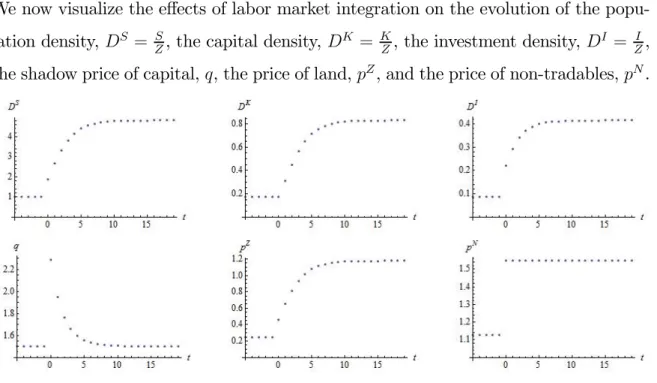
Labor Market Integration

We now visualize the effects of labor market integration on the evolution of the popu-lation density,  ₌ 

, the capital density, 

 ₌ 

, the investment density, 

 ₌ 

,

the shadow price of capital, , the price of land, _{, and the price of non-tradables, }_.

Figure 2 (a): The impact of labor market integration in period = 0on a high-productivity economy which initially has the same population density as abroad and is in steady state.

Note:  =  = 55,∗ _{= }∗ _{= 5, } 0 = ˜  (₋₁ ), and  −1= ∗= 1  ˜  .

In Fig. 2 (a), the economy is initially in its pre-labor-market-integration steady state, which corresponds to the case in part (i) of Proposition 4. Moreover, we assume that, initially, the population density coincides with that of the foreign economy, ₋₁ = ∗ _{= 1. Productivity levels are, however, 10 percent higher compared to the foreign}

economy, i.e. _∗ =



∗ = 11. That is, the initial population density is below its

post-integration long run level, 

−1  ˜, and the initial capital density reads 0 =

˜

(₋₁ ). This constellation may be interpreted as the case of an advanced country which opens up the labor market. As we will argue in section 6, an appropriate example which can be discussed in the light of our model is the case of Switzerland which opened the labor market to the EU in the 2000s.

Now, when the labor market is opened up in period  = 0, the population density, _{, jumps upwards and then gradually increases along with the capital density. The}

migration inflow, induced by a comparably high domestic wage rate, raises the demand for non-tradables and triggers an increase in the price of non-tradables, , as well as an increase in the price of land, _{. The upward jump in } _{represents a drag on further}

migration inflows. In line with part (iii) of Proposition 4,  _{instantaneously jumps to}

its new steady state level, as displayed in the last panel of Fig. 2 (a). Also the shadow value of installed capital, , goes up, fostering higher investment. Consequently, the capital stock rises.

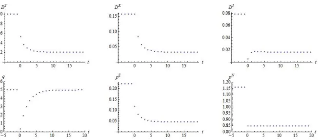
Figure 2 (b): The impact of labor market integration in period  = 0on a high-productivity economy which initially has the same population density as abroad and is in steady state.

Note:  =  = 5,∗ = ∗ = 55, 0 = ˜ 

(₋₁ ), and ₋₁= ∗= 1  ˜.

In Fig. 2 (b), as before, the economy is initially in its pre-labor-market-integration steady state and 

−1 = ∗ = 1. Productivity levels are now about 10 percent lower

compared to the foreign economy, i.e. _∗ =



∗ ∼= 09. That is, the initial population

density is below its post-integration long run level, 

−1  ˜, and the initial capital

density reads 0 = ˜(−1 ). When the labor market is opened up in period

 = 0, the population density, _{, jumps downwards and then gradually declines}

along with the capital density. The migration outflow, induced by a comparably low domestic wage rate, reduces the demand for non-tradables and triggers a decrease

in the price of non-tradables, _{, as well as a decrease in the price of land, }_{. The}

downward jump in  represents a drag on further migration outflows. Also the shadow value of installed capital, , goes down, fostering lower gross investment such that net investment turns negative. Consequently, the capital stock declines. In sum, if the initial capital stock is at the pre-labor-market-integration steady state level, we observe emigration (immigration), lower (higher) house and land prices, and capital decumulation (accumulation) at the same time.

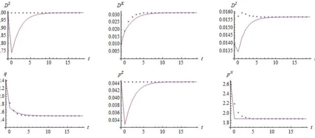
Figure 3: Solid lines show dynamic responses assuming labor market integration at  = 0

for an initially capital-poor economy with the same population density as abroad. Dotted lines show dynamic responses assuming that labor markets remain closed. Note:

 = ∗=  = ∗= 5,0  ˜ 

( ˜ ),₋₁ = ˜.

We now assume that domestic productivity levels are equal to the foreign economy, i.e.,  = ∗ _{and  = }∗_{. Eq. (19) then implies that the post-integration long run}

popu-lation density coincides with that of the foreign economy, ˜ = ∗ = 1. The initial population density is also equal to this value (

−1 = ∗), while the capital density

is lower than the post-integration value, 0  ˜( ˜ ). The solid time paths of

Fig. 3 illustrate economic development provided that the labor market is opened up at  = 0. The dotted lines show, in contrast, economic development under the alternative

assumption of closed labor markets. Fig. 3 (solid lines) illustrates part (ii) of Proposi-tion 4, i.e., the possibility that emigraProposi-tion may go along with capital accumulaProposi-tion after labor markets integrate. We see that the population density considerably falls below ∗ _{= ˜} _{immediately after the integration shock. Therefore, also the shadow value}

of capital drops, leading to a lower investment density, _{. Nevertheless, as  is still}

above its steady state level, which reflects the standard neoclassical convergence force, there is still capital accumulation. Over time, and after the immediate response of 

to integration, population density rises along with capital accumulation. This explains why the land price, _{, rises after its initial drop. The price of the non-tradable good,}

, again jumps immediately to the new steady state level. As argued in the discussion of part (iii) of Proposition 4, the effect of the gradually increasing  _{and } _{on }

cancel out such that  _{remains unchanged below its pre-integration level during the}

transition. This case provides a candidate explanation for reverse migration, which coincides, for instance, with the recent experience in Poland and East Germany. Turn-ing to the alternative scenario of closed labor markets (dotted lines), we see that 

remains constant,  is much higher, compared to the case of labor market integration and resulting emigration, such that capital gets accumulated more quickly. The land price, _{, does not drop and the price for non-tradables, }_{, declines gradually, which}

reflects the absence of emigration.10

It is worth noting that reverse migration cannot be explained by standard neoclas-sical models (Rappaport, 1995; Burda, 2006). Technically, the difference between our model and standard neoclassical models of migration and capital mobility based on some form of convex adjustment costs for both capital and labor is that, in our model, labor is a jump variable determined by the no-arbitrage condition  (   +1) = ∗

(see Definition 1) and not a sluggish state variable (e.g., Braun, 1993; Rapapport, 2005). 10_{Notice that this does not contradict Proposition 4 (iii), which assumes that the labor market is}

opened up such that (18) holds. This is not the case for the scenario represented by the dotted lines in Fig. 3.

5

Distribution of Land and Welfare

For simplicity, we have so far assumed that land is not owned by individuals in the domestic economy. Moreover, the previous analysis suggests that the price of the non-tradable good is higher than its initial level at all times after a shock which induces labor inflows. Thus, if individuals earn labor income only, the native population necessarily loses from immigration, according to (10).

In this section, by contrast, we assume that initially land is fully owned by the ₋₁ old natives. Landowners bequeath their landholding to their child when leaving the scene, such that the number of landowners and the land distribution among natives is time-invariant. Let () denote the landholding of individual . For the sake of realism, suppose that a non-negligible fraction of natives is landless (for such an individual , () = 0).

In period , a young individual  who stays in the domestic economy has a present discounted value of life-time income, (), which is given by

() =  +

 +1

1 + () (21) (recall that the wage rate is  =  and land is owned by old individuals). Life-time

utility of individual  born in  is  (()   +1), where function  is given by (10).

5.1

Equilibrium Analysis

We again start with the case where population density is exogenous. The dynamic system modifies as follows.

Proposition 5. _{Suppose that the sequence of population density {}

}∞=0 is given.

(i) The capital density ( 

 ), the investment density ( ), the shadow value of

capital ( ), the price of the non-tradable good (  ), and the price of land ( ) jointly

(1_{− )}+1 = (1 + ) −  µ  +1  +1 ¶+1 − _+1¡_+1 ¢−1 ∙  (1_{− )}  (1 + ) ¡ _+1+ ¡_+2+ _+1¢¢ ¸  (22) _ = 1  ³   ´µ_{1− } 1 +  ¶1−_£ (_+1+ _) + _¤1−¡_ ¢− (23) +1 = 1  µ 1 +  (1_{−  − ) (1 − )} −  ¶  −     (24)

(ii) If  is time-invariant, then, in the long run, the price of land, the capital density, and the price of the non-tradable good are respectively given by11

 = ˜ _(_{ )} 1_{− 2} ≡ ˆ _(_{ ) (25)}  = ˜ _(_{ )} 1_{− 2} ≡ ˆ _(_{ ) (26)}  = µ 1 1_{− 2} ¶1−− ˜ (  )_{≡ ˆ}(  ) (27) Comparing Proposition 5 with Proposition 1, the dynamics appear more compli-cated than in the case where natives do not own land. The reason is that individuals who own land have to anticipate the future price of land.

Comparison with Proposition 1 also reveals that, in the long run, the price of land (), the capital density () and the price of non-tradables () are higher than in the case where nobody owns land: ˆ _{ ˜}_{, ˆ} _{ ˜}_{, ˆ} _{ ˜}_{. The key ingredient}

of the model which gives rise to this result is the declining marginal productivity of land: if natives receive land rents in addition to wage income, this raises the demand for all goods. However, since land is a fixed factor, it becomes more scarce. This raises the price of land along with house prices. As a consequence of the latter, incentives to

11_{Recall from part (i) of Proposition 1 the parameter definition  =} (1−−)(1−)

1+ . Note that

accumulate capital are higher as well.

Note that the distribution of land does not affect the dynamic system. The reason lies in the assumption of homothetic preferences, which implies that aggregate goods demand is independent of the income distribution.

We now turn to the equilibrium analysis for the case of interregionally mobile labor.

Lemma 2. When landless individuals are indifferent whether or not to migrate, no landowner wants to migrate.

Lemma 2 suggests that the incentive to migrate is higher for landless individuals. The reason is simple. Land rents are received from the home region irrespective of the location decision, whereas wage income depends on the chosen location. Thus, income-related migration benefits come from wage differentials only. Differences in the log of income across regions are therefore higher for landless individuals. We focus on an equilibrium where only (some) landless individuals migrate. For such an equilibrium to exist, the share of landless individuals has to be sufficiently large. In this case, the no-arbitrage condition (18) for the migration decision (equilibrium condition 3 of Definition 1) still holds, where now the price of non-tradables abroad is given by  ∗ _{= ˆ}_(∗

 ∗_{ }∗_{). Consequently, the steady state population density is still given}

by (19) such that Corollary 1 applies. Thus, the implications on structural estimations, discussed in subsection 3.3, still apply.

Moreover, if we conduct the same experiments as for Fig. 2 and 3, the dynamics triggered by an integration shock are qualitatively the same as in the case where no individual owns land (available on request). That is, if labor markets are opened when the economy is in steady state initially, population density (_{), capital density (}_),

and prices for both non-tradables () and land () move into the same direction (Fig. 2). When the economy is not in steady state at the time labor markets integrate, population density and capital density may move in different directions instantaneously in response to integration (Fig. 3).

5.2

Welfare

We now analyze the effects of labor market integration on individual welfare, condi-tional on land endowment. For the long run, we find the following result.

Proposition 6. If labor market integration leads to an increase in the long run population density, landowners of the steady state generations win if and only if they own a sufficient amount of land; landless individuals lose.

Proposition 6 suggests an important distributional impact of immigration which is different from effects on the distribution of labor income often discussed in the literature. If housing demand increases in response to immigration, both land rents of landowners and the price of housing increase.12 _{If and only if the land estate of}

an individual is sufficiently high, the positive effect of immigration on land income dominates. Thus, there is a threshold amount of landholding, ¯  0, such that all individuals with ()  ()¯ win (lose) from labor market integration.

We now discuss welfare effects of integration over time for non-steady state gener-ations. To do so, we need to compare the time paths of house prices and land prices with and without integrated labor markets. Recall that house prices immediately jump to the new steady state level after labor market integration. In the scenario where the pre-integration capital stock was initially at the steady state level and population den-sity was low to begin with, the land price rises over time (Fig. 2). Thus, the threshold land endowment ¯ above which an individual gains from immigration falls over time. As consumers, individuals lose from integration in any period. But as the stock of immigrants rises, later generations of landowners earn higher income than earlier ones. When the economy is initially capital-poor, labor market integration leads to em-igration and retarded capital accumulation (Fig. 3). Also recall that the land price drops initially in response to integration but, in contrast to house prices, rises after-wards as the migration flow reverses. Without migration, the land price would have 12_{As discussed after Proposition 1, there are also two counteracting supply effects of immigration on}

the price of land, which cancel each other. First, when more houses are built, land becomes scarcer. This raises land prices for given house prices. Second, however, house prices decline. This has a depressing effect on the value of the marginal product of land.

been constant over time whereas the house price would have fallen gradually without integration due to capital accumulation. Thus, in the scenario of Fig. 3, where the steady states with and without migration coincide, we can conclude that non-steady state generations of landless individuals are better off with integration. Non-steady state generations of rich landowners, however, may lose during the transition.

6

The Case of Switzerland

Without exaggeration, immigration is one of the most debated issues in the Swiss public in the last 10 years and beyond. Switzerland is an interesting case because it is a high-wage country which has experienced a substantial labor market integration shock. In the year 2002, it signed a bilateral agreement with the European Union on the free movement of labor. With respect to the EU15 plus Malta and Cyprus, referred to as EU17 in the following, it came into full effect in 2007.13 _{This exogenous event}

in a small high-wage country serves as a kind of "natural experiment" to "test" the predictions of our model as visualized in Fig. 2 (a). (Recall that, in Fig. 2 (a), we study the impact of labor market integration on an economy with high productivity and an initial capital density which coincides with the pre-labor-market-integration steady state level).

Fig. 4 shows the annual net migration inflow into Switzerland from the year 2002 to 2010 by the region of origin. The integration process provoked net immigration from the EU17 at first to slightly increase after 2002, jumping upwards after 2007. In the "control group" of non-EU17 countries, net immigration shows only a slight upward trend. Consistent with the first panel in Fig. 2 (a), which displays the population density as a strictly concave function during the transition to the new steady state after labor markets integrate, net migration inflows decreased after the initial jumps 13_{Between 2002-2006, immigration to Switzerland was only slightly facilitated. Like before,}

residents were still preferred in the labor market, meaning that a potential employer had to prove that the firm does not find an adequate resident for the job. Moreover, immigration quotas were held in place. For most Eastern European countries free movement of labor has come into effect in May 2011. Burgaria and Romania even have to wait until mid 2016. See http://www.bfm.admin.ch/content/bfm/en/home/themen/fza_schweiz-eu-efta.html

in 2007 and 2008.

Figure 4: Net immigration flow to Switzerland (annual number of immigrants minus number of emigrants) between 2002-2010 from EU17 and non-EU17 countries. (Source:

bfs.admin.ch; own calculations)

Figure 5: Rental price index for Switzerland, monthly data, offer-based. (Source: ZKB, Zürcher Kantonal Bank; www.zkb.ch)

Moreover, rental prices for houses and apartments in Switzerland started to increase in 2004 and rose by 20 percent between 2002 and 2010, as displayed by Fig. 5.14 _This

sluggish price increase is not readily compatible with the transitional dynamics for the price of housing, , derived from our basic model. Fig. 2 (a) suggests that  jumps immediately to a higher steady state level in response to integration. However, the absence of transitional dynamics in  _{hinges on the simplifying assumption that only}

labor enters the production function of the tradable good (

 = ). Allowing for

capital as a second input in the tradable goods sector modifies the transition path of _{. Let }

 denote the stock of capital employed in the tradable goods sector. We

maintain a constant-returns to scale technology and modify the production function to

_ = ¡_¢¡_¢1−, (28)  _{∈ (0 1). Conducting the same experiment as in Fig. 2 (a), Fig. 6 shows that }

(left panel) increases smoothly during the transition to the new steady state. The price of non-tradable goods, , drops initially because the wage rate, , falls at  = 0 in response to migration inflows, as displayed in the right panel. This reduces the demand for the non-tradeable good, as can be seen from (9) and  = . The reduction in

the wage rate is, however, not persistent since the wage converges back to its initial steady state value, despite further massive immigration. This behavior of the wage rate is consistent with empirical evidence which, if anything, suggests a short-run drop in the wage rate and negligible long-run effects (e.g. Friedberg, 2001; Borjas, 2003; Dustmann et al., 2005). The underlying reason for the increase in  along the smooth transition is that firms, in both sectors, build up their capital stock because a larger labor force makes installed capital goods more valuable. All other properties of the transition paths are qualitatively similar to Fig. 2 (a).

is no official house price index in Switzerland. However, the Zürcher Kantonalbank, a local bank based in Zurich, publishes estimates based on own sales transactions data and data from an internet platform for buying and renting houses and appartments (www.zkb.ch).

Figure 6: The impact of labor market integration in period = 0under the same presumptions as in Fig. 2 (a), except that the production technology for the tradable good

is modified to (28) with = 05.

From Fig. 4 and 5 one also recognizes that rental prices started to increase (in 2004) before net immigration started to increase (in 2006). This observation is in line with our theory by noting that the Swiss labor market integration represents an expected integration shock. We kept the analysis deliberately as simple as possible by assuming an unexpected integration shock. Hence, the timing of events in the data (i.e., the price increase first, then the increase in net immigration rates) can easily be reconciled with our theory.

A sceptic may ask whether the observed magnitude of migration inflows can plau-sibly be held responsible for the rental price increase. Two aspects are noteworthy in this regard. An annual (net) migration inflow of 100 thousand people, like in the year 2008 where Switzerland had 7.7 million inhabitants, amounted to a 1.4 percent increase of the domestic population. Although this increase does not sound dramatic at the first glance, these migration inflows were highly concentrated in urban areas. For instance, the residential population in the canton of Zurich increased by about 9.1 percent between 2006 and 2011. The sales price index for residential property during this period rose by about 30 percent (data source: http://www.zkb.ch).

The considerably rising prices for housing services have provoked an intensive debate on the gains from migration in Switzerland. At the first glance, this seems remarkable as wage effects are barely visible and a large fraction of immigrants from EU countries

is tertiary educated. The debate seems reasonable, however, in view of our model. In particular, and consistent with the welfare effects suggested by Proposition 6, the association of tenants but not those of house owners have recently opposed further immigration. This indicates that immigration to Switzerland has triggered a new distributional conflict, which dominates recent policy and media debates. Previous debates on migration have centered on wage effects and the implications of low-skilled migration on the social policy system. Recently, by contrast, not only populist right-wing parties but also left-right-wing parties and interest groups argue in favor of sloright-wing down or even reversing migration flows. All important opponents to immigration started focussing on rental rates of housing.15 The parties in the middle do not express strong views. In the light of our model, this could be rationalized by the fact that their constituency is particularly heterogenous in terms of their land- and houseownership.

7

Conclusion

This paper has examined the impact of labor market integration on migration, capital formation, house prices, and land prices in an intertemporal model in which firms face capital adjustment costs. Our theory is compatible with no or weak wage effects. The mechanism which acts as a drag on migration flows and prevents that everyone moves to high-productivity regions, once this is legally made feasible, works through changes in the price of housing. The predictions of our model are, for instance, in line with the recent experience of Switzerland after integration of its labor market to the European labor market.

We have examined how initial conditions (i.e., initial levels of population density, productivity, and the capital stock) affect the direction and evolution of migration and capital flows over time. In particular, our theory provides a candidate explanation for reverse migration. According to the best of our knowledge, previous studies based on 15_{According to our analysis, redistribution of land or wealth, or more indirect redistribution}

mea-sures from rich landowners to poorer individuals, would be a way to spread the gains of landowners from immigration to a wider population. This points to the possibility that, from a normative point of view, redistribution measures may be preferable to reversing labor market integration.

neoclassical models which rest on constant returns to scale did not explain that labor market integration may lead to labor outflows in early phases of the transition to the new long run equilibrium and immigration in later phases. In our model, the number of people in the domestic economy is determined by the condition that life-time utility in the source and the destination are equalized. As a result, technically, population density is a jump variable which allows for non-monotonic transitions in a natural and intuitive way.

At a normative level, the paper has shown how heterogeneity of landownership determines the distributional consequences in response to labor market integration, caused by changes in the rental rate of land. This may help to understand political debates on and resistance to immigration even if immigration has negligible effects on the wage distribution.

As regards future research, we suggest to introduce externalities, implying that the aggregate output technologies exhibit increasing returns to scale, such that multiple equilibria may emerge. This modification could then be employed to examine how initial conditions and expectations interact for the dynamic evolution of migration, capital formation, house prices, and land prices.

Appendix

Proof of Lemma 1. The household’s problem is solved in two steps. In the first step, the intertemporal consumption problem is solved. Omitting subscripts, define a Cobb-Douglas consumption index,  :=¡¢¡_¢1− _{such that instantaneous utility}

is given by log . Consumption expenditure in a given period can be expressed as

  =  +  (29) where  denotes an appropriately defined price index (see below). Life-time utility of an individual born in  reads as  = log 1+  log 2+1.

individ-ual born in  in the first and second period of life by 1and 2+1, respectively.

First-period income is equal to the wage rate, 1 = . (Moreover, in the basic model, 2 ≡ 0.)

Let  denote individual savings in working age at time , i.e., := − 11.

We have 1= −  1  (30) 2+1 = (1 + ) + 2+1 2+1  (31)

The intertemporal problem may be expressed as follows:

max

 {log (

− )− log (1) +  log [(1 + ) + 2+1]−  log (2+1)}  (32)

Defining ≡ +

2+1

1+ , the first-order condition implies

1= 1 1 +  (33) 2+12+1 1 +  =  1 +  (34) In the second step, we analyze the static problems. Given the amount of first period consumption expenditure when young in , 1= _1+1 , the household solves

max  11 logh¡_1¢¡_1¢1−i s.t. 1 1 + =   1+      1 (35) Hence, _1 =  1_{− }     1 (36)

which combined with _1+1 = 1+  1 implies

_1=  1 +    1= 1_{− } 1 +      (37)

 + 1, 2+12+1= (1+)_1+ , the household solves max  2+12+1 logh¡2+1 ¢¡ 2+1 ¢1−i s.t.  (1 + ) 1 +  =   2+1+ +12+1 (38) Hence, we get 2+1=  1_{− }  +1  2+1 (39)

which combined with (1+)_1+ = 2+1+ +12+1 leads to

_2+1=  (1 + )  1 +     2+1 = (1_{− ) (1 + ) } 1 +    +1  (40)

Substituting (1 + )  = 1 and inserting the goods demand functions into the intertem-poral utility function confirms (8)-(10). It remains to be shown that there exists a price index as used above. Using  =¡¢¡_¢1−_{, the price index  may be expressed as}

 =   _{+ }_  = µ   ¶1− +  µ   ¶  (41) Noting that _ =  1−  _{one gets}  =¡¢1− "µ  1_{− } ¶1− + µ 1_{− }  ¶#  (42)

This concludes the proof. ¥

Proof of Proposition 1. The Lagrangian function to the optimization problem (3) of firms in sector  , implied by equilibrium condition 1 in Definition 1, is given by

L = ∞ X =0 µ 1 1 +  ¶µ   ¡  ¢ ()  1−− _{− } −  −  ∙ 1 +  µ   ¶¸ + [+ (1− ) − +1])  (43)

Using = , the associated first-order conditions _L  = L  = L  = L +1 = 0 imply _ =  ¡   ¢1−  ()1−−  (44) _ = _ (1_{−  − ) }¡_¢()−− (45) = µ − 1 ( + 1)  ¶1   (46) (1_{− )}+1+ +1 ¡ _+1¢(+1)−11−− +  µ_ +1  +1 ¶+1 = (1 + ) (47) Recall  ₌   and   ₌ 

. Then, first, (46) gives us (12). Substituting (46)

into (2) confirms (11). Substituting (1) as well as 

1 and 2 as given by (9) into

equilibrium condition 6 in Definition 1, 

 = 1 + 2−1, and using  =  implies ¡_ ¢()1−− = 1_{− } 1 +     (+ −1) (48)

Substituting (44) into (48) and solving for 

 we obtain

_ = (1− )

1 +  (+ −1) (49) Advancing (49) by one period and using it in (47), as well as recalling  ₌ 

,

 ₌ 

, 

 ₌ 

, and  = + −1 confirms (13). Moreover, substituting (49) into

(44) confirms (14). Substituting (44) into (45) and using (49) confirms (15).

We next show that, for a given population density (_{), the system (11)-(13) is}

saddle-point stable. To see this, use (12) in (11) to find

∆_+1:= _+1 _{− } = "µ − 1 ( + 1)  ¶1  −  # _  (50) Thus, ∆+1 is increasing in . Moreover, the locus which is given by ∆+1 = 0 in