HAL Id: inria-00536363
https://hal.inria.fr/inria-00536363
Submitted on 16 Nov 2010
HAL is a multi-disciplinary open access
archive for the deposit and dissemination of sci-entific research documents, whether they are pub-lished or not. The documents may come from teaching and research institutions in France or abroad, or from public or private research centers.
L’archive ouverte pluridisciplinaire HAL, est destinée au dépôt et à la diffusion de documents scientifiques de niveau recherche, publiés ou non, émanant des établissements d’enseignement et de recherche français ou étrangers, des laboratoires publics ou privés.
Quantifying the Sub-optimality of Uniprocessor Fixed
Priority Non-Pre-emptive Scheduling
Robert Davis, Laurent George, Pierre Courbin
To cite this version:
Robert Davis, Laurent George, Pierre Courbin. Quantifying the Sub-optimality of Uniprocessor Fixed Priority Non-Pre-emptive Scheduling. 18th International Conference on Real-Time and Network Sys-tems, Nov 2010, Toulouse, France. pp.1-10. �inria-00536363�
Quantifying the Sub-optimality of Uniprocessor Fixed Priority Non-Pre-emptive
Scheduling
Robert I. Davis
Real-Time Systems Research
Group,
Department of Computer Science,
University of York, York, UK.
rob.davis@cs.york.ac.uk
Laurent George
AOSTE Team, INRIA
Rocquencourt, BP 105,
Domaine de Voluceau, 78153,
Le Chesnay Cedex, France
lgeorge@ieee.org
Pierre Courbin
Ecole Centrale d'Electronique
de Paris (ECE), LACSC,
37 Quai de Grenelle,
75015 Paris, France
courbin@ece.fr
Abstract
This paper examines the relative effectiveness of fixed priority non-pre-emptive scheduling (FP-NP) in a uniprocessor system, compared to an optimal work-conserving non-pre-emptive algorithm; Earliest Deadline First (EDF-NP). The quantitative metric used in this comparison is the processor speedup factor, defined as the factor by which processor speed needs to increase to ensure that any taskset that is schedulable according to EDF-NP can be scheduled using FP-NP scheduling. For sporadic tasksets with implicit, constrained, or arbitrary deadlines, the speedup factor is shown to be lower bounded by 1/Ω≈1.76322 and upper bounded by 2.
We also report the results of empirical investigations into the speedup factor required to ensure schedulability in the non-pre-emptive case.
1. Introduction
In this paper, we are interested in determining the largest factor by which the processing speed of a uniprocessor needs to be increased, to ensure that any taskset that was previously schedulable according to an optimal work-conserving (i.e. non-idling), non-pre-emptive scheduling algorithm is schedulable according to fixed priority non-pre-emptive (FP-NP) scheduling. We refer to this resource augmentation factor as the processor speedup factor [17].
1.1. Pre-emptive scheduling
In 1973, Liu and Layland [22] considered fixed priority pre-emptive (FP-P) scheduling of synchronous1
tasksets comprising independent periodic tasks, with bounded execution times, and deadlines equal to their periods. We refer to such tasksets as implicit-deadline tasksets. Liu and Layland showed that rate monotonic priority ordering (RMPO) is the optimal fixed priority assignment policy for implicit-deadline tasksets, and that using rate monotonic priority ordering, FP-P can schedule any implicit-deadline taskset that has a total utilisation U ≤ln(2)≈0.693.
Liu and Layland [22] also showed that Earliest Deadline First (EDF-P) is an optimal dynamic priority
1A taskset is synchronous if all of its tasks share a common release
time.
pre-emptive scheduling algorithm for implicit-deadline tasksets, and that EDF-P can schedule any such taskset that has a total utilisation U ≤1.
In 1974, Dertouzos [9] showed that EDF-P is an optimal uniprocessor scheduling algorithm, in the sense that if a valid schedule exists for a taskset, then the schedule produced by EDF-P will also meet all deadlines.
Research into real-time scheduling during the 1980’s and early 1990’s focussed on lifting many of the restrictions of the Liu and Layland task model. Task arrivals were permitted to be sporadic, with known minimal inter-arrival times, (still referred to as periods), and task deadlines were permitted to be less than or equal to their periods (so called constrained deadlines) or less than, equal to, or greater than their periods (so called arbitrary deadlines).
In 1982, Leung and Whitehead [19] showed that deadline monotonic2 priority ordering (DMPO) is the optimal fixed priority ordering for constrained-deadline tasksets. Exact schedulability tests for FP-P scheduling of constrained-deadline tasksets were introduced by Joseph and Pandya in 1986 [16], Lehoczky et al. in 1989 [21], and Audsley et al. in 1993 [1].
In 1990, Lehoczky [20] showed that DMPO is not optimal for tasksets with arbitrary deadlines; however, an optimal priority ordering for such tasksets can be determined in at most n(n+1)/2 task schedulability tests using Audsley’s optimal priority assignment (OPA) algorithm3 [1], [2]. Exact schedulability tests for tasksets
with arbitrary deadlines were developed by Lehoczky [20] in 1990 and Tindell et al. [23] in 1994.
Exact EDF-P schedulability tests for both constrained and arbitrary-deadline tasksets were introduced by Baruah et al. [3], [4] in 1990.
1.2. Non-pre-emptive scheduling
In 1980, Kim and Naghibdadeh [18], and in 1991, Jeffay et al. [15], gave exact schedulability tests for implicit-deadline tasksets under Earliest Deadline First non-pre-emptive (EDF-NP) scheduling. These tests were
2 Deadline monotonic priority ordering assigns priorities in order of
task deadlines, such that the task with the shortest deadline is given the highest priority.
3This algorithm is optimal in the sense that it finds a schedulable
extended by George et al. [12] in 1996, to the general case of sporadic tasksets with arbitrary deadlines.
While EDF-P is an optimal uniprocessor scheduling algorithm, in the non-pre-emptive case no work-conserving algorithm is optimal. This is because in general it is necessary to insert idle time to achieve a feasible schedule. The interested reader is referred to [12] for examples of this behaviour.
In 1995, Howell and Venkatrao [14] showed that for non-concrete4 periodic tasksets, the problem of
determining a feasible non-pre-emptive schedule is NP hard. Further they showed that for sporadic tasksets, no optimal on-line inserted idle time algorithm can exist. In other words, clairvoyance is needed to determine a feasible non-pre-emptive schedule.
While no work-conserving algorithm is optimal in the strong sense that it can schedule any taskset for which a feasible non-pre-emptive schedule exists; in 1995, George et al. [13] showed that EDF-NP is optimal in the weak sense that it can schedule any taskset for which a feasible work-conserving, non-pre-emptive schedule exists. Hence we can regard EDF-NP as an optimal work-conserving, non-pre-emptive scheduling algorithm, for non-concrete tasksets.
George et al. [12] derived an exact schedulability test for fixed priority non-pre-emptive (FP-NP) scheduling of arbitrary-deadline tasksets, based on the approach of Tindell et al. [23] for the pre-emptive case. George et al. showed that unlike in the pre-emptive case, deadline monotonic priority ordering is not optimal for constrained-deadline tasksets scheduled by FP-NP. Further, they showed that Audsley’s optimal priority assignment algorithm [2] is applicable, and can be used to determine an optimal priority ordering for tasksets with arbitrary-deadlines scheduled using FP-NP.
Subsequent research by Bril et al. [5] has refined exact analysis of FP-NP, correcting issues of both pessimism and optimism, and extending the schedulability tests to co-operative scheduling where each task is made up of a number of non-pre-emptive sections.
1.3. Sub-optimality and speedup factors
Combining the result of Dertouzos [9] with the results of Liu and Layland [22], shows that the processor speedup factor required to guarantee that FP-P scheduling can schedule any implicit-deadline taskset schedulable by EDF-P is 1/ln(2)≈1.44270.
In 2009, Davis et al. [7] derived the exact speedup factor for FP-P scheduling of constrained-deadline tasksets; 1/Ω≈1.76322 (where Ω is the mathematical constant defined by the transcendental equation
Ω = Ω) / 1 ln( , hence, Ω≈0.567143). Also in 2009, Davis et al. [8] showed that the speedup factor for FP-P scheduling of arbitrary-deadline tasksets is lower bounded by 1/Ω≈1.76322 and upper bounded by 2. Further, if deadline monotonic priority assignment is assumed (which is not optimal for arbitrary-deadline tasksets), then the exact speedup factor required is 2.
4A periodic taskset is referred to as non-concrete if the times at which
each task is first released are unknown.
In this paper, we derive upper and lower bounds on the speedup factor required such that any taskset that was previously schedulable according to an optimal work-conserving (i.e. non-idling) non-pre-emptive scheduling algorithm (i.e. EDF-NP) can be guaranteed to be schedulable according to fixed priority non-pre-emptive (FP-NP) scheduling. These bounds are valid for all three classes of non-concrete taskset; Implicit-deadline, constrained-Implicit-deadline, and arbitrary-deadline. While these results are mainly theoretical, they also have practical utility in enabling system designers to quantify the maximum penalty for using fixed priority non-pre-emptive scheduling in terms of the additional processing capacity required. This performance penalty can then be weighed against other factors such as implementation overheads when considering which scheduling algorithm to use.
1.4. Organisation
The remainder of this paper is organised as follows. Section 2 describes the system model, notation and analysis used. Section 3 illustrates the concept of processor speedup factors via a simple example. Section 4 derives a lower bound on the processor speedup factor required for FP-NP scheduling, while Section 5 derives the corresponding upper bound. Section 6 reports on an empirical investigation into the speedup factor required for FP-NP scheduling, verifying the theoretical lower bound. Section 7 concludes with a summary of the results and suggestions for future work.
2. System model, notation, and analysis
In this section, we outline the scheduling model, notation and terminology used in the rest of the paper. We then recapitulate schedulability analysis for both FP-NP and EDF-FP-NP scheduling.2.1. Scheduling model, terminology and notation
In this paper, we consider the non-pre-emptive scheduling of a set of sporadic tasks (or taskset) on a uniprocessor.
Each taskset comprises a static set of n tasks (τ1..τn), where n is a positive integer. We assume that the index i of task τ also represents the task priority used in fixed i priority scheduling, hence τ has the highest fixed-1 priority, and τ the lowest. n
Each task τ is characterised by its bounded worst-i case execution time Ci, minimum inter-arrival time or period Ti, and relative deadline Di. Each task τ i therefore gives rise to a potentially infinite sequence of invocations (or jobs), each of which has an execution time upper bounded by Ci, an arrival time at least Ti after the arrival of its previous invocation, and an absolute deadline Di time units after its arrival.
In an implicit-deadline taskset, all tasks have i
i T
D = . In a constrained-deadline taskset, all tasks haveDi≤Ti, while in an arbitrary-deadline taskset, task deadlines are independent of their periods, thus each task may have a deadline that is less than, equal to, or greater than, its period. The set of arbitrary-deadline tasksets is therefore a superset of the set of constrained-deadline tasksets, which is itself a superset of the set of implicit deadline tasksets.
The utilisation Ui, of a task is given by its execution time divided by its period (Ui=Ci/Ti). The total
utilisation U, of a taskset is the sum of the utilisations of all of its tasks:
∑
= = n i i U U 1 (1)The following assumptions are made about the behaviour of the tasks:
o The arrival times of the tasks are independent and unknown a priori (non-concrete), hence the tasks may share a common release time.
o Each task is released (i.e. becomes ready to execute) as soon as it arrives.
o The tasks are independent and so cannot block each other from executing by accessing mutually exclusive shared resources, with the exception of the processor.
o The tasks do not voluntarily suspend themselves.
A task is said to be ready if it has outstanding computation awaiting execution by the processor.
A taskset is said to be schedulable with respect to some scheduling algorithm and some system, if all valid sequences of task invocations (or jobs) that may be generated by the taskset can be scheduled on the system by the scheduling algorithm without any deadlines being missed.
Under EDF-NP scheduling, whenever a job completes execution, or when the processor is idle and a job becomes ready to execute, the ready job with the earliest absolute deadline is selected to execute. By contrast, under FP-NP the highest priority ready job is selected.
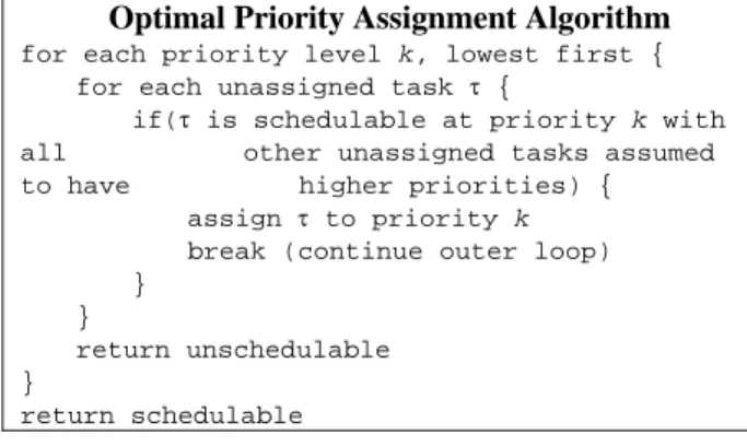
When a taskset is scheduled according to FP-NP, task priorities need to be assigned according to some algorithm. Audsley’s Optimal Priority Assignment (OPA) algorithm [1], [2], (see Figure 1 below) provides the optimal policy for sporadic tasksets with implicit-deadlines, constrained-deadlines or arbitrary-deadlines.
Optimal Priority Assignment Algorithm for each priority level k, lowest first {
for each unassigned task τ {
if(τ is schedulable at priority k with
all other unassigned tasks assumed
to have higher priorities) {
assign τ to priority k
break (continue outer loop) }
}
return unschedulable
}
return schedulable
Figure 1: OPA algorithm
A priority assignment policy P is said to be optimal with respect to some class of tasksets, and a fixed priority scheduling algorithm FP-X if there are no tasksets in the class that are schedulable according to FP-X using any other priority ordering policy that are not also schedulable using the priority assignment determined by policy P.
A taskset is said to be feasible with respect to a given
system model if there exists some scheduling algorithm that can schedule all possible sequences of task activations that may be generated by the taskset on that system without missing any deadlines.
A scheduling algorithm is said to be optimal with respect to a system model and a tasking model if it can schedule all of the tasksets that comply with the tasking model and are feasible on the system.
We note that EDF-NP is optimal in the weak sense that it can schedule any sporadic taskset for which feasible work-conserving, non-pre-emptive schedules exist [13].
A schedulability test is termed sufficient, with respect to a scheduling algorithm and system model, if all of the tasksets that are deemed schedulable according to the test are in fact schedulable on the system under the scheduling algorithm. Similarly, a schedulability test is termed necessary, if all of the tasksets that are deemed unschedulable according to the test are in fact unschedulable on the system under the scheduling algorithm. A schedulability test that is both sufficient and necessary is referred to as exact.
2.2. Schedulability analysis for FP-NP
Exact schedulability analysis for an arbitrary-deadline sporadic taskset under FP-NP was given by George et al. [12] and Bril et al. [5]. Below, we provide a simple sufficient schedulability test for FP-NP scheduling, derived from these exact tests. This sufficient test is used in the derivation of an upper bound on the speedup factor for FP-NP scheduling given in Section 5. First, we introduce the concepts of worst-case response time, priority level-i active period, and ∆-critical instant, which are fundamental to analysis of FP-NP scheduling.
For a taskset scheduled under FP-NP scheduling, the worst-case response time Ri of a task τ is given by the i longest possible time from release of the task until it completes execution. Thus task τ is schedulable if and i only if Ri≤Di, and the taskset is schedulable if and only if ∀i Ri ≤Di.
The term priority level-i active period refers to a continuous period of time [t1,t2) during which tasks, of priority i or higher, that were released at the start of the active period at t1, or during the active period but strictly before its end at t2, are either executing or ready
to execute.
A ∆-critical instant for a task τ refers to a pattern of i task arrivals such that task τ is released simultaneously i with all tasks of higher priority than i, and then subsequent releases of task τ and the higher priority i tasks occur as early as possible given the constraints on minimum inter-arrival times. Further, some infinitesimal amount of time ∆ prior to this simultaneous release, a lower priority task τ is released, and this task has the k longest execution time of any such lower priority task. Thus the longest time that task τ and higher priority i tasks can be blocked from executing by lower priority tasks is given by : ⎪⎩ ⎪ ⎨ ⎧ = < Δ − = ∀∈ n i n i C Bi k lpi k 0 ) ( max ) ( (2)
where lp(i) is the set of tasks with priorities lower than i. Bril et al. [5] showed that for FP-NP scheduling, the longest response time of a task τ occurs for some i invocation of the task within the priority level-i active period starting at the ∆-critical instant for task τ . i Lemma 3 in [5] states that the worst-case length of a priority level-i active period Ai is given by the minimum solution to the following fixed point iteration:
j i hep j j m i i m i T C A B A
∑
∈ ∀ + ⎥ ⎥ ⎥ ⎤ ⎢ ⎢ ⎢ ⎡ + = ) ( 1 (3)where hep(i) is the set of tasks with priorities higher than or equal to i. Iteration starts with an initial value Ai0
guaranteed to be no larger than the minimum solution, for example Ai0 =Ci, and ends when m
i m i A
A +1 = . From Equation (3), we can form the following simple sufficient test for FP-NP scheduling of arbitrary-deadline tasksets. Each task τ is schedulable provided that: i
k i hep k k i i i T C D B D
∑
∈ ∀ ⎥ ⎥ ⎥ ⎤ ⎢ ⎢ ⎢ ⎡ + ≥ ) ( (4) If Equation (4) holds, then this indicates that the solution to the fixed point iteration of Equation (3) must be ≤Di. As the worst-case length of a priority level-i active period is then ≤Di, it follows that the worst-case response time Ri of task τ must also be i ≤Di, andhence the task must be schedulable. If all of the tasks are schedulable according to Equation (4), then the taskset is schedulable. (For an exact schedulability test for FP-NP, see [5]).
2.3. Schedulability analysis for EDF-NP
Baruah et al [3], [4] gave an exact schedulability test for EDF-P based on the concept of the processor demand bound function h(t). George et al. [12] extended this test to EDF-NP via the addition of a blocking factor B(t).
i n i i i C T D t t h
∑
= ⎟ ⎟ ⎠ ⎞ ⎜ ⎜ ⎝ ⎛ + ⎥ ⎦ ⎥ ⎢ ⎣ ⎢ − = 1 1 , 0 max ) ( (5) ⎪⎩ ⎪ ⎨ ⎧ ≥ < Δ − = ∀ ∀ > ∀ ) ( max 0 ) ( max ) ( max ) ( : i i i i i t D i D t D t C t B i (6)George et al. [12] showed that an arbitrary-deadline taskset is schedulable under EDF-NP if and only if
1 ≤
U and a quantity referred to as the processor LOAD is ≤1, where the processor LOAD is given by:
LOAD ⎟ ⎠ ⎞ ⎜ ⎝ ⎛ + = ∀ t t B t h t ) ( ) ( max (7)
Further, if U ≤1 and the value of (h(t)+B(t))/t is ≤1
for all values of t in the interval ( L0, ], (where L is the length of the synchronous priority level-n active period, given by the minimum solution to Equation (3)), then LOAD ≤1. Thus the only values of t that need to be checked are those in the interval ( L0, ] that correspond to times when h(t)+B(t) can change, i.e.
i i D
kT t
i = +
∀ for integer values of k. We note that recently significant developments have been made, reducing the number of values of t that need to be checked [11]; however, this simple description of the analysis is sufficient for the purposes of this paper. (We
note that for schedulable tasksets, the maximum value of
t t B t
h() ())/
( + does not necessarily occur in the interval
] , 0
( L , but does occur in the interval [Dmin,H] where
min
D is the shortest task deadline and H is the taskset hyperperiod or Least Common Multiple of task periods [10]).
2.4. Definitions
Definition 1: Let fOPT(Ψ) be the lowest processor speed such that taskset Ψ is schedulable according to an optimal scheduling algorithm. Assume that f A(Ψ) is
similarly the lowest processor speed that will schedule taskset Ψ using scheduling algorithm A. The processor speedup factor f A for algorithm A is given by the maximum increase in processor speed required over an optimal algorithm for any taskset Ψ.
(
( )/ ( ))
max Ψ Ψ = Ψ ∀ OPT A A f f f (8)For any scheduling algorithm A, we have f A ≥1, with smaller values of f A indicative of a more effective scheduling algorithm, and fA =1 implying that A is an
optimal algorithm.
In the remainder of the paper, unless otherwise stated, when we refer to the processor speedup factor, we mean the processor speedup factor for FP-NP scheduling using an optimal priority assignment policy, as compared to EDF-NP, an optimal (in the weak sense [13]), work-conserving non-pre-emptive scheduling algorithm. Definition 2: A taskset is said to be speedup-optimal if it requires the processor to be speeded up by the processor speedup factor in order to be schedulable using FP-NP scheduling. Hence for a speedup-optimal taskset Ψ ,
A OPT
A f f
f (Ψ)/ (Ψ)= .
Definition 3: Let S be some arbitrary taskset, now assume that αFP−NP(S) is the maximum factor by which the execution times of all of the tasks in S can be scaled, such that the taskset is schedulable under FP-NP. Similarly, let αEDF−NP(S) be the maximum scaling factor under EDF-NP. The speedup factor
) (S
fFP−NP for the taskset is given by:
) ( / ) ( ) (S S S fFP−NP =αEDF−NP αFP−NP (9)
3. Example
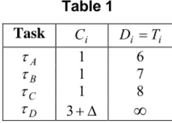
The concept of a speedup factor for a given taskset S can be illustrated by means of the following example. Consider the taskset S comprising the tasks defined in Table 1, with priorities assigned in the order that the tasks appear in the table (i.e. τ has the highest priority, A and τ the lowest). D
Table 1 Task C i Di =Ti A τ 1 6 B τ 1 7 C τ 1 8 D τ 3+Δ
∞
The worst-case arrival pattern for tasks τ , A τ , and B τ C under FP-NP scheduling is shown in Figure 2. Note the 1st job of each task is shaded in grey, while the 2nd job of
Figure 2: FP-NP schedule
Now consider the maximum factor by which the execution times of the tasks can be scaled and the taskset remain schedulable according to FP-NP. This factor is
− −NP(S)=(6/5) FP
α (i.e. a value infinitesimally less than 6/5).
Figure 3: FP-NP schedule, maximal scaling Figure 3 shows the FP-NP schedule for the scaled taskset. Scaling by any larger factor, for example, a factor equal to 6/5 would result in the first job of task
C
τ being unable to start executing before the 2nd job of
task τ is released at time t = 6. It would then be further A delayed by the 2nd job of task
B
τ , and hence fail to met its deadline at time t = 8. In fact, there is no priority ordering which results in taskset S, scaled by a factor of 6/5, being schedulable. This can be seen by considering the behaviour of the OPA algorithm. While task τ is D schedulable at the lowest priority, and can therefore be assigned priority 4, none of the other tasks are schedulable at priority 3.
Figure 4: EDF-NP schedule, maximal scaling With EDF-NP scheduling, the maximum scaling factor commensurate with taskset S remaining schedulable is αEDF−NP(S)=8/6. Under EDF-NP, the first job of task τ has a later absolute deadline than the C first jobs of tasks τ and A τ , and therefore executes B
after those jobs and after the first job of τ which is D released at time t=−Δ. The first job of task τ is not C
however delayed by the 2nd jobs of tasks
A
τ and τ , as B these jobs have later absolute deadlines. With a scaling factor of 8/6, the first job of task τ just completes by C its deadline (see Figure 4). Further analysis is required to prove that the scaled taskset is schedulable under EDF-NP; however, as the priority level 3 active period ends at
12 =
t , we need only check all deadlines in the interval
[0, 12] to show schedulability. Note, Figure 4 shows the ∆-critical instant for tasks τ , A τ , B τ , and all deadlines C
are met in the interval [0, 12]. Further, task τ is D trivially schedulable as it has an infinite deadline, and the taskset utilisation is less than 1.
Using Equation (9), the speedup factor for the taskset given in Table 1 is fFP−NP(S) = (8/6)/(6/5)− = + ) 36 / 40
( = (10/9)+ (i.e. a value infinitesimally larger than 10/9). In the next section, we generalise this example and show how tasksets with a similar structure but with a large number of tasks require a much larger speedup factor.
4. Lower bound speedup factor for FP-NP
In this section, we derive a lower bound on the processor speedup factor required for FP-NP scheduling using optimal priority assignment [1], [2]. This lower bound is valid for sporadic and non-concrete periodic tasksets with implicit-, constrained-, and arbitrary-deadlines. In Section 5, we derive an upper bound with the same scope.To derive a lower bound, we need only select a single taskset and determine the required speedup factor for that taskset. The taskset S that we use is a generalisation of the taskset used as an example in Section 3. In this case, there are n tasks, with the parameters given in Table 2. Tasks τ to 1 τn−1 are represented by τ in the i first row of the table. All of these tasks have the same small execution time ε<< X , and related periods/deadlines. Further, all of the tasks have periods equal to their deadlines, so this is an implicit-deadline taskset. Task τ has an execution time of n X +Δ, where X is a free variable that we can alter to maximise the required speedup factor.
Table 2 Task Ci Di =Ti i τ ) 1 ( 1 − = n ε ) 1 ( ) 1 ( 1 − − + + n i X n τ X+Δ
∞
The execution of taskset S under FP-NP is depicted in Figure 5 below. Note, jobs of task τn−1 are marked with
an ε .
Figure 6: FP-NP schedule, maximal scaling Lemma 1: The maximum factor αFP−NP(S) by which the execution times of the tasks in taskset S (Table 2) can be scaled and the taskset remain schedulable according to FP-NP. is given by: + → − − ⎟ = ⎠ ⎞ ⎜ ⎝ ⎛ − + + = 1 1 1 ) ( 0 ε ε α X X S NP FP (10) Figure 6 depicts the FP-NP schedule for the scaled taskset.
Proof: Scaling by a factor equal to (1+X)/(1+X+ε) would result in the first job of task τn−1 being unable to
start executing before the 2nd job of task
1
τ is released at time t= 1+X It would then be further delayed by the 2nd jobs of tasks
1
τ to τn−2, and hence fail to met its deadline at time t=2+X −ε. In fact, there is no priority ordering which results in taskset S, scaled by a factor of (1+X)/(1+X +ε), being schedulable. This can be seen by considering the behaviour of the OPA algorithm, given the scaled taskset: Task τ is n
schedulable at the lowest priority, and can therefore be assigned that priority. However, considering the remaining tasks in turn, none of them are schedulable at priority n-1. Task τ is not schedulable at priority n-1, as 1 its 1st job would miss its deadline at t= 1+X . Task
2
τ is not schedulable at priority n-1, as its 1st job is then
unable to start before the 2nd job of task
1
τ arrives, and so misses its deadline at t=1+X +ε . In general, with a scaling factor of (1+X)/(1+X +ε), for each task with index i from 2 to n-1, assuming that task τ is assigned i priority n-1, ensures that the 1st job of task
i
τ is unable to start before the 2nd job of task
1 −
i
τ arrives, and so the 1st job of task
i
τ misses its deadline.
By contrast, with a scaling factor of
−
+ + + )/(1 ) 1
( X X ε , task τn−1 is schedulable at priority n-1, as it is able to start executing just prior to the arrival of the 2nd job of
1
τ at t= 1+X . Further, with this scaling factor, all of the other tasks are schedulable with priorities assigned according to their indices (i.e. in Deadline Monotonic priority order). This can be seen by checking the deadlines of all jobs up to the end of the priority level n-1 active period, which occurs at:
− ⎟ ⎠ ⎞ ⎜ ⎝ ⎛ + + + + = ε X X X tA 1 ) 1 ( ) 2 ( (11)
As tA<2(1+X)=2D1, the priority level n-1 active period comprises the 1st job of task
n
τ and the 1st and 2nd
jobs of tasks τ to 1 τn−1. All of these are schedulable
(see Figure 6). The priority level-n active period is of similar length, and hence task τ is trivially schedulable n given its infinite deadline □
Lemma 2: The maximum factor αEDF−NP(S) by which
the execution times of the tasks in taskset S (Table 2) can be scaled and the taskset remain schedulable according to EDF-NP. is given by:
− −NP(S)=(1/Ω) EDF
α (12)
Proof: There are two key conditions which limit the maximum scaling factor under EDF-FP (otherwise the taskset would become unschedulable):
1. The 1st jobs of all tasks must be complete by the
deadline of task τn−1, Dn−1=2+X −ε.
2. Utilisation of the scaled taskset must not exceed 100%.
Considering the first condition, we have:
X X S NP EDF + − + ≤ − 1 2 ) ( ε α (13)
The utilisation of the un-scaled taskset is given by the sum of the utilisation of each task:
) 1 1 1 ( 1 ) 1 ( 1 1 1 − − + + − =
∑
− = n i X n U n i (14)The RHS of Equation (14) is recognisable as the left Riemann sum of the function 1/z, over the interval
) 2 , 1 [ +X +X , hence: ⎟ ⎠ ⎞ ⎜ ⎝ ⎛ + + = = +
∫
+ ∞ → X X dz z U X X n 1 2 ln 1 2 1 (15)Thus, considering the second condition, we have:
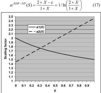
⎟ ⎠ ⎞ ⎜ ⎝ ⎛ + + ≤ − X X S NP EDF 1 2 ln / 1 ) ( α (16)
As Equation (13) is monotonically non-increasing in X and tends to 2 for small X, and Equation (16) is monotonically non-decreasing in X and tends to 1/ln(2) for small X, then the maximum value is obtained when the RHSs of Equations (13) and (16) are equal, i.e. when: = + − + = − X X S NP EDF 1 2 ) ( ε α ⎟ ⎠ ⎞ ⎜ ⎝ ⎛ + + X X 1 2 ln / 1 (17) 1 1.1 1.2 1.3 1.4 1.5 1.6 1.7 1.8 1.9 2 2.1 2.2 2.3 2.4 2.5 0 0.1 0.2 0.3 0.4 0.5 0.6 0.7 0.8 0.9 X S cal in g f a ct or a1(X) a2(X)
Figure 7: Constraints on the scaling factor as a function of X
Figure 7 plots Equations (13) and (16) (labelled a1(X) and a2(X) respectively) against X. As n→∞, ε→0,
the solution to Equation (17) is given by the intersection of the lines plotted in Figure 7, thus
76322 . 1 ) / 1 ( ) ( = Ω − ≈ −NP S EDF α , (where Ω is the
mathematical constant defined by the transcendental equation ln(1/Ω)=Ω, hence, Ω≈0.567143). Further,
310232 . 0 1 1 2 ≈ Ω − − − Ω = ε X (18)
We now show that taskset S (Table 2) is schedulable under EDF-NP, when scaled by a factor of
− −NP(S)=(1/Ω) EDF
α . Proof is made significantly
easier by the commonality between taskset S and the speedup-optimal taskset V for the constrained-deadline case of FP-P scheduling, described in Theorem 2 of [7]. In fact, tasks τ to 1 τn−1 are identical in these two
tasksets, only task τ differs. In taskset V, the n parameters of task τ are: n Cn=X , Dn= 2+X , and
∞ =
n
T , whereas in taskset S, the parameters of task τ n are: Cn = X+Δ, and Dn =Tn =∞ Theorem 4 in [7]
proves that taskset V is schedulable under EDF-P when scaled by a factor of 1/Ω. Hence for taskset V,
1 ) ( max ⎟≤ ⎠ ⎞ ⎜ ⎝ ⎛ = ∀ t t h LOAD t P (19)
We make use of this result to show that taskset S, scaled by a factor of (1/Ω)− is schedulable under EDF-NP. As tasks τ to 1 τn−1 are identical, their contribution to the processor demand bound h(t) is the same for any time t. We now compare the contribution from task τ n in each case. In the pre-emptive case, (taskset V), τ n contributes to h(t) as follows: ⎩ ⎨ ⎧ + ≥ Ω + < ≤ = ) 2 ( / ) 2 ( 0 0 ) ( X t X X t t hnP (20)
whereas, in the non-pre-emptive case, (taskset S), τ n contributes only to the blocking factor:
0 ) / ( ) (t = X Ω − t≥ B (21) Recall that in the non-pre-emptive case, a taskset is schedulable provided that U ≤1 and:
1 ) ( ) ( max ⎟≤ ⎠ ⎞ ⎜ ⎝ ⎛ + = ∀ t t B t h LOAD t NP (22)
Comparing Equations (19) and (22), and the contributions of task τ in each case (Equations (20) and n (21)), it follows that Equation (22) holds for all values of
) 2
( X
t≥ + for taskset S scaled by a factor of (1/Ω)−. This is because, for all values of t≥(2+X) the value of
t t B t
h() ())/
( + is the same as that for taskset V, assuming both tasksets are scaled by the same factor. To prove the schedulability of taskset S scaled by a factor of
−
Ω) / 1
( , it remains only to show that (h(t)+B(t))/t≤1 for all values of t in the interval [0,(2+X)). Here, we need only check values of t that correspond to task deadlines. As 2+X >2D1, this amounts to checking the 1st deadline of each of the n-1 highest priority tasks. At
each of these deadlines Di, we have:
1 1 1 , 0 max 1 ) ( 1 1 ⎟ − ⎟ ⎠ ⎞ ⎜ ⎜ ⎝ ⎛ ⎟ ⎟ ⎠ ⎞ ⎜ ⎜ ⎝ ⎛ + ⎥ ⎦ ⎥ ⎢ ⎣ ⎢ − ⎟ ⎠ ⎞ ⎜ ⎝ ⎛ Ω =
∑
− = − n T D D D h n k k k i i (23) as ∀ ,i k Di =Ti and Di <2Dkit follows that:1 1 ) ( − ⎟ ⎠ ⎞ ⎜ ⎝ ⎛ Ω = − n i D h i (24) Hence the scaled taskset is schedulable provided that,
i ∀ from 1 to n-1, Di ≥h(Di)+B(Di) ⎟ ⎠ ⎞ ⎜ ⎝ ⎛ − + ⎟ ⎠ ⎞ ⎜ ⎝ ⎛ Ω ≥ − − + + − 1 1 1 1 1 n i X n i X (25) Substituting for (1/Ω)− =(2+X−ε)/(1+X) and
) 1 /( 1 − = n
ε , and rearranging, we have:
⎟ ⎠ ⎞ ⎜ ⎝ ⎛ − + ⎟ ⎠ ⎞ ⎜ ⎝ ⎛ − − + ≥ + ⎟ ⎠ ⎞ ⎜ ⎝ ⎛ − − + + 1 1 1 2 ) 1 ( 1 1 1 n i X n X X n i X (26) which simplifies to:
0 ) 1 ( 1 2 1 1 1 2 ≥ − + − − − − + n i n i n i (27) and then to:
0 ) 1 ( 1 2 2 ≥ − + − − − n i n i n (28)
For n≥2, the first term in inequality (28) is non-negative ∀i from 1 to n-2, while the second term is always positive. Further, for i = n-1, the first and second terms cancel out, thus the inequality holds ∀i from 1 to n-1. Taskset S is therefore schedulable according to EDF-NP when scaled by a factor of (1/Ω)− □
Theorem 1: A lower bound on the speedup factor required for FP-NP scheduling of an implicit-deadline taskset is: − + − − − − = = Ω =(1/Ω) 1 ) / 1 ( ) ( ) ( S S f FP NP NP EDF NP FP α α (29) Proof: Follows from Lemmas 1 and 2 and the definition of the speedup factor □
Corollary 1: We observe that as taskset S is an implicit-deadline taskset, and all implicit-implicit-deadline tasksets are also constrained-deadline and arbitrary-deadline tasksets, the lower bound of Theorem 1 applies to all three classes of taskset.
It remains an open question whether or not the lower bound given in Theorem 1 is tight. While the taskset used to derive the bound is valid, whether or not it is a speedup optimal taskset (see Definition 2) remains to be proved / disproved. If the bound is not tight, then there exists a different taskset construction that requires a larger speedup factor.
5. Upper bound speedup factor for FP-NP
In this section, we derive an upper bound on the speedup factor required for FP-NP scheduling of arbitrary-deadline sporadic and non-concrete periodic tasksets.Theorem 2: An upper bound on the processor speedup factor required such that FP-NP scheduling, using optimal priority assignment can schedule any arbitrary-deadline sporadic or non-concrete periodic taskset schedulable under EDF-NP according to Equation (7), is 2.
Proof: Let S be any taskset that is schedulable according to Equation (7) on a processor of unit speed under EDF-NP. For each task τ , in S, consider the processor k demand bound and blocking factor for an interval of length 2Dk. As taskset S is schedulable according to EDF-NP, it follows that:
k i n i i i k k T C D D D D B(2 ) max 0, 2 1 2 1 ≤ ⎟ ⎟ ⎠ ⎞ ⎜ ⎜ ⎝ ⎛ ⎟ ⎟ ⎠ ⎞ ⎜ ⎜ ⎝ ⎛ + ⎥ ⎦ ⎥ ⎢ ⎣ ⎢ − +
∑
= (30) Next, consider taskset S scheduled according to FP-NP scheduling on a processor of speed 2 using Deadline Monotonic priority assignment (rather than OPA). DMPO implies that ∀i≤k Di≤Dk .From Equation (30) above, assuming speed 2, and separating out the contribution from all tasks of lower or equal priority to k we have:
+ ⎟ ⎟ ⎠ ⎞ ⎜ ⎜ ⎝ ⎛ + ⎥ ⎦ ⎥ ⎢ ⎣ ⎢ − +
∑
∈lepk i i i i k k T C D D D B ) ( 1 2 , 0 max ) 2 ( k i k hp i i i k C D T D D ≤ ⎟ ⎟ ⎠ ⎞ ⎜ ⎜ ⎝ ⎛ + ⎥ ⎦ ⎥ ⎢ ⎣ ⎢ −∑
∈ ( ) 1 2 , 0 max (31)where lep(k) is the set of tasks with priorities lower than or equal to k. As the tasks are in DMPO, we note that all of the tasks in lep(k) have deadlines ≥Dk.
We now consider just the first and second terms in Equation (31). Observe that the contribution to the second term from every task τ in i lep(k)
withDi >2Dk is zero. Further, there is a contribution from each task τ with i Dk ≤Di ≤2Dk of at least Ci. From the definition of B(t) (Equation (6)), the definition of Bk (Equation (2)), and the fact that the
tasks are in DMPO, it follows that the sum of the first two terms in Equation (31) are ≥Bk, the blocking factor for FP-NP scheduling: k D D D i i i i k i i k i D D i C B D D D D C k i k k i + ≥ ⎪⎭ ⎪ ⎬ ⎫ ≥ < Δ −
∑
≤ ≤ ∀ ∀ ∀ > ∀ 2 : 2 : ) ( max 2 0 ) ( max 2 ) ( max where ⎪⎩ ⎪ ⎨ ⎧ = < Δ − = ∀∈ n k n k C Bk i lpk i 0 ) ( max ) ( (32) Substituting Bk for the first two terms in Equation (31) and transforming the third term by noting that⎣ ⎦
x +1≥⎡ ⎤
x and ∀i∈hp(k) Di≤Dk we have: k i k hp i i k k T C D D B ⎥ ≤ ⎥ ⎤ ⎢ ⎢ ⎡ +∑
∈ ( ) (33)Equation (33) is identical to Equation (4); the sufficient schedulability test for task τ in an arbitrary-deadline k taskset S, scheduled under FP-NP. Repeating the above argument for each task τ in S therefore proves that the k taskset is schedulable on a processor of speed 2 under FP-NP, with Deadline Monotonic priority assignment. As optimal priority assignment for FP-NP can schedule any taskset that is schedulable using FP-NP with Deadline Monotonic priority ordering □
Corollary 2: We observe that as the upper bound in
Theorem 2 holds for arbitrary-deadline tasksets, it must also hold for implicit-deadline, and constrained-deadline tasksets.
6. Empirical results
In this section, we confirm by experiment the results presented in Section 4 concerning the lower bound speedup factor for FP-NP. We consider the task set proposed in Table 2 where n−1 tasks have worst-case execution times equal to 1/(n−1), and task τ has a n worst-case execution time equal to X+Δ and an infinite period and deadline.
Our experiments indicate that a value of X ≈0.31
results in the maximum speedup factor for a given number of tasks. Based on this value, we verify the lower bound given in this paper for a large number of tasks.
Taskset S investigated in this section is based on the task model presented in Table 2. This model is theoretical, while our empirical assumptions are as follows:
o Δ is equal to 0.001.
o The infinite values of period and deadline for task τ are replaced in the experiments by n values such that τn does not interfere with other tasks.
Finally, to avoid the problem of rounding, we have used integer values, thus given that Δ is the time granularity, each task parameter {Ci,Di,Ti} is normalized according to Δ. For example, with three tasks and X = 1, Table 3 gives the task set studied.
Table 3: Example of taskset studied with
001 . 0 = Δ and X =1 Task Ci Di =Ti 1 τ 500 2000 2 τ 500 2500 3 τ 1001 ∞
In order to determine the speedup factor fFP−NP(S), we compute the maximum factors αEDF−NP(S) and
) (S
NP FP−
α via an approach based on binary search (dichotomy). Algorithm 1 describes this approach, as used in our experiments. To check the schedulability of task set S, the function checkFeasibility() uses following exact tests: • For EDF-NP [12]: 1 ) ( ) ( max ] , 0 [ ⎟⎠≤ ⎞ ⎜ ⎝ ⎛ + ∈ ∀ t t B t h L t (34) • For FP-NP [6]: i i i q i Q q i W C qT D R i i < − + = ∀ ∈max ( ) , , ] , 0 [ max (35) where max =
⎡
/⎤
−1 i i i A T Q , Ai is computed according to Equation (3) and Wi,q is given by the minimum solution to the following fixed point iteration:i i i m q i m q i T C B W W + ⎥ ⎥ ⎥ ⎤ ⎢ ⎢ ⎢ ⎡ +Δ = +1 , , (36)
with Bi determined by Equation (2) and Wi0q =qTi
, .
Finally, the speedup factor is computed via Equation (9) f FP−NP(S)=αEDF−NP(S)/αFP−NP(S).
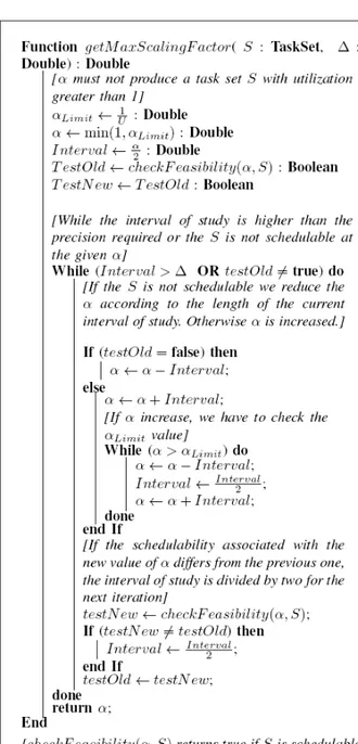
Algorithm 1: Determines the maximum scaling factor of a taskset S with a precision Δ via
binary search (dichotomy).
Figure 8 shows the maximum speedup factor obtained for n=5 tasks. It shows the value of X for which the speedup factor was empirically found to be a maximum i.e. X =0.31.
Figure 9 represents, for this optimum value
31 . 0
=
X , the speedup factor obtained as a function of the number of tasks (from 10 to 400 tasks). We observe that the maximum speedup factor for FP-NP tends towards 1.76322, the lower bound of fFP−NP(S)
characterized in Section 4, as the number of tasks increases. Note that the saw tooth appearance of the curve is an artefact of the quantisation of the execution time values used in the experiment. When the number of tasks is large, this causes a noticeable quantisation of the scaling factors that can be explored.
Figure 8: Constraints on the scaling factor as a function of X for n=5 1.76322 1.2 1.3 1.4 1.5 1.6 1.7 1.8 0 100 200 300 400 Number of tasks S p e e du p f act or f o r F P -N P Lower Bound Speedup factor (Empirical value)
Figure 9: Speedup factor for X =0.31 as a function of the number of tasks
7. Conclusions and future work
In this paper, we examined the relative effectiveness of fixed priority non-pre-emptive scheduling. Our metric for measuring the effectiveness of this scheduling algorithm is a resource augmentation factor known as the processor speedup factor. In this case, the processor speedup factor is defined as the minimum amount by which the processor needs to be speeded up so that any taskset that is schedulable by an optimal work-conserving non-pre-emptive scheduling algorithm (e.g. EDF-NP) can be guaranteed to be schedulable under FP-NP scheduling. Recall that EDF-FP-NP is optimal in the weak sense [13], in that it can schedule all sporadic or concrete periodic tasksets for which a feasible non-pre-emptive, work-conserving schedule exists. It is not optimal in the strong sense as it cannot schedule all tasksets for which a feasible work-conserving, non-pre-emptive schedulable exists. The speedup factors derived in this paper are with respect to this weak form of optimality.
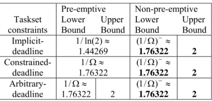
Table 4: FP scheduling speedup factors Pre-emptive Non-pre-emptive Taskset
constraints Lower Bound Upper Bound Lower Bound Upper Bound Implicit-deadline 11.44269 /ln(2)≈ Ω ≈ − ) / 1 ( 1.76322 2 Constrained-deadline ≈ Ω / 1 1.76322 ≈ Ω)− / 1 ( 1.76322 2 Arbitrary-deadline ≈ Ω / 1 1.76322 2 ≈ Ω)− / 1 ( 1.76322 2
Table 4 shows the processor speedup factor needed for fixed priority scheduling with optimal priority assignment, for both the pre-emptive case (FP-P v. EDF-P), see Davis et al. [7], [8], and for the non-pre-emptive case (FP-NP v. EDF-NP), derived in this paper.
The major contribution of this paper is in proving that the processor speedup factor for fixed priority non-pre-emptive scheduling of sporadic or non-concrete periodic tasksets with optimal priority assignment, is upper bounded by 2, and lower bounded by (1/Ω)− = 1.76322. We note that these bounds hold for tasksets with implicit-, constrained-, and arbitrary-deadlines.
The seminal work of Liu and Layland [22] characterises the maximum performance penalty incurred when an implicit-deadline taskset is scheduled using Rate-Monotonic, fixed priority pre-emptive scheduling instead of an optimal algorithm such as EDF-P. The research in this paper provides an analogous characterisation of the maximum performance penalty incurred when tasksets are scheduled using fixed priority non-pre-emptive scheduling instead of an optimal work-conserving non-pre-emptive scheduling algorithm e.g. EDF-NP.
We note that the two cases in Table 4 where a tight bound is known correspond to the only cases where optimal priority assignment can be achieved independently of schedulability testing. In the arbitrary-deadline case for P scheduling and all cases of FP-NP scheduling, Audsley’s OPA algorithm is required to find the optimal priority ordering. This dependence of priority ordering on schedulability testing makes it more difficult to reason about the properties of a theoretical speedup-optimal taskset that requires the exact speedup factor to be schedulable. In these cases, the exact sub-optimality of fixed priority scheduling remains an open question.
7.1. Acknowledgements
This work was funded in part by the EPSRC project TEMPO (EP/G055548/1) and the EU funded ArtistDesign Network of Excellence. The authors would like to thank Alan Burns for his insightful comments on an earlier draft.
References
[1] Audsley N.C., "Optimal priority assignment and feasibility of static priority tasks with arbitrary start times", Technical Report
YCS 164, Dept. Computer Science, University of York, UK, 1991.
[2] Audsley N.C. “On priority assignment in fixed priority scheduling”, Information Processing Letters, 79(1): 39-44, May 2001.
[3] Baruah S.K., Mok A.K., Rosier L.E., “Preemptively Scheduling Hard-Real-Time Sporadic Tasks on One Processor”. In
Proc. RTSS, pages182-190, 1990.
[4] Baruah S.K., Rosier L.E., Howell R.R., “Algorithms and Complexity Concerning the Preemptive Scheduling of Periodic Real-Time Tasks on one Processor”. Real-Time Systems, 2(4), pages 301-324, 1990.
[5] Bril, R.J., Lukkien, J.J., and Verhaegh, W.F., “Worst-case response time analysis of real-time tasks under fixed-priority scheduling with deferred pre-emption”. Real-Time Systems. 42, 1-3 (Aug. 2009), 61-3-119.
[6] Davis, R. I., Burns, A., “Controller area network (CAN) schedulability analysis: Refuted, revisited and revised,” Real-Time Systems, vol. 35, pp. 239–272, 2007.
[7] Davis R.I., Rothvoß T., Baruah S.K., Burns A., “Exact Quantification of the Sub-optimality of Uniprocessor Fixed Priority Pre-emptive Scheduling.” Real-Time Systems, Volume 43, Number 3, pages 211-258, November 2009.
[8] Davis, R.I., Rothvoß, T., Baruah, S.K., Burns, A., “Quantifying the Sub-optimality of Uniprocessor Fixed Priority Pre-emptive Scheduling for Sporadic Tasksets with Arbitrary Deadlines”. In proceedings of Real-Time and Network Systems
(RTNS'09), pages 23-31, October 26-27th, 2009.
[9] Dertouzos M.L., “Control Robotics: The Procedural Control of Physical Processes”. In Proc. of the IFIP congress, pages 807-813, 1974.
[10] Fisher, N., Baker, T. P., Baruah, S. “Algorithms for Determining the Demand-Based Load of a Sporadic Task System”. In Proceedings of the 12th IEEE international Conference on
Embedded and Real-Time Computing Systems and Applications
(RTCSA), pages 135-146, 2006.
[11] George, L., Hermant, J., “A norm approach for the Partitioned EDF Scheduling of Sporadic Task Systems.” In Proc. ECRTS, 2009.
[12] George, L., Rivierre, N., Spuri, M., “Preemptive and Non-Preemptive Real-Time UniProcessor Scheduling”, INRIA Research Report, No. 2966, September 1996.
[13] George, L., Muhlethaler, P., Rivierre, N., “Optimality and Non-Preemptive Real-Time Scheduling Revisited,” Rapport de Recherche RR-2516, INRIA, Le Chesnay Cedex, France, 1995. [14] Howell, R.R., Venkatrao, M.K., “On non-preemptive scheduling of recurring tasks using inserted idle time”, Information and computation Journal, Vol. 117, Number 1, Feb. 15, 1995. [15] K. Jeffay, D. F. Stanat, C. U. Martel, “On Non-Preemptive Scheduling of Periodic and Sporadic Tasks”, In Proc. RTSS, pages 129-139, 1991.
[16] Joseph M., Pandya P.K., “Finding Response Times in a Real-time System”. The Computer Journal, 29(5), pages 390–395, 1986. [17] Kalyanasundaram B., Pruhs K., “Speed is as powerful as clairvoyance”. In Proceedings of the 36th Symposium on
Foundations of Computer Science, pages 214-221, 1995.
[18] Kim, Naghibdadeh, “Prevention of task overruns in real-time non-preemptive multiprogramming systems”, Proc. of Perf., Assoc. Comp. Mach., 1980, pp 267-276.
[19] Leung J.Y.-T., Whitehead J., "On the complexity of fixed-priority scheduling of periodic real-time tasks". Performance
Evaluation, 2(4), pages 237-250, 1982.
[20] Lehoczky J., “Fixed priority scheduling of periodic task sets with arbitrary deadlines”. In Proc. RTSS, pages 201–209, 1990. [21] Lehoczky J.P., Sha L., Ding Y., “The rate monotonic scheduling algorithm: Exact characterization and average case behaviour”. In Proc. RTSS, pages 166–171, 1989.
[22] Liu C.L., Layland J.W., "Scheduling algorithms for multiprogramming in a hard-real-time environment", Journal of
the ACM, 20(1) pages 46-61, 1973.
[23] Tindell K.W., Burns A., Wellings A.J., “An extendible approach for analyzing fixed priority hard real-time tasks”.