HAL Id: hal-03105551
https://hal.archives-ouvertes.fr/hal-03105551
Submitted on 11 Jan 2021
HAL is a multi-disciplinary open access archive for the deposit and dissemination of sci-entific research documents, whether they are pub-lished or not. The documents may come from teaching and research institutions in France or abroad, or from public or private research centers.
L’archive ouverte pluridisciplinaire HAL, est destinée au dépôt et à la diffusion de documents scientifiques de niveau recherche, publiés ou non, émanant des établissements d’enseignement et de recherche français ou étrangers, des laboratoires publics ou privés.
Do slum upgrading programmes improve living
standards? Evidence from Djibouti
Sandrine Mesplé-Somps, Laure Pasquier-Doumer, Charlotte Guénard
To cite this version:
Sandrine Mesplé-Somps, Laure Pasquier-Doumer, Charlotte Guénard. Do slum upgrading pro-grammes improve living standards? Evidence from Djibouti. European Journal of Development Research, 2020, �10.1057/s41287-020-00305-9�. �hal-03105551�
Do slum upgrading programmes improve employment?
Evidence from Djibouti
Forthcoming in The European Journal of Development Research
2020, July
Sandrine Mesplé-Somps,1 DIAL, LEDa, IRD, Université Paris-Dauphine, Université PSL, 75016 Paris, France, [email protected]
Laure Pasquier-Doumer, DIAL, LEDa, IRD, Université Paris-Dauphine, Université PSL,75016 Paris, France, [email protected]
Charlotte Guénard, UMR Développement and Sociétés, Université Paris 1-IEDES, IRD, JATP, 94736 Nogent-sur-Marne, France, [email protected]
Abstract
Slum upgrading programmes are high on the international community’s agenda. Yet their impact evaluations remain few and far between, especially when the programmes include different components such as roads, water supply, electricity, and community facilities. In addition, employment is rarely considered as an outcome in the evaluation of slum upgrading programmes, although it is often one of the main priorities of slum upgrading policies. This article analyses the effects on employment of such a programme in a Djibouti slum. It uses a difference-in-difference approach to evaluate the average impact and heterogeneous effects of the programme. We find that the project is unlikely to have improved access to employment in general and to formal wage jobs in particular, as was expected at the start of the project. It has also failed to increase earned income. Nonetheless, we show that self-employed activities have developed, more particularly in places adjacent to the project roads.
Keywords: slums, urban project, impact analysis, employment, Djibouti. JEL: R23, J68
1
2 Introduction
Over one-third of the urban population in developing countries lives in slums (UN-Habitat, 2013). The proportion is estimated to be much higher in Sub-Saharan Africa, at over two-thirds of the urban population. In addition, the downward trend observed in these indicators since 2000 is slower in Sub-Saharan Africa than in developing countries as a whole.
After several decades of urban planning policies around the world, urban specialists have now largely demonstrated the undesirable effects of certain public urban planning policies. As summarized by Clerc, Criqui and Josse (2017), "destruction and re-housing often displace inhabitants away from the centres, while the supply of public or assisted housing remains vacant or benefits the upper classes. Social housing or subsidised private constructions exist, but are often unsuitable: outlying, quickly abandoned, without job prospects, poorly connected to transport, lacking social ties."
As opposed to functionalist town planning, it is now accepted that an "urban project" whose aims (defined in consultation with inhabitants) are to "rehabilitate and improve in situ working-class neighbourhoods with support for self-construction, provision of services, public spaces, land regularization, etc. is more appropriate than policies of tabula rasa and the creation of new housing neighbourhood ex nihilo" (Clerc, Criqui and Josse, 2017). Slum upgrading – also known as in situ rehabilitation – projects are still high on the international community’s agenda.
Slum upgrading projects vary from small, single-sector interventions to integrated programmes comprising many activities and targeting different problems at the same time. Integrated programmes generally provide basic services such as water supply, electricity, wastewater drainage, waste disposal, roads, and the construction of community facilities. They also sometimes include social programmes ranging from vocational training to land
3
titling programmes. Integrated programmes were implemented early on in Latin American cities such as Mexico City, Lima, and Medellin, as pointed out by Deboulet (2016). The development of these programmes is rooted in the assessment of the limitations of relocation programmes and the necessity to implement in situ programmes (Jaitman, 2015), but also in the idea that only a combination of actions can achieve the outcomes targeted (Jaitman and Brakarz, 2013).
In spite of their growing popularity, quantitative evaluations of such projects remain few and far between (Marx et al., 2013). One reason is that integrated slum upgrading programmes do not lend themselves well to experimental methods. Their multiple components mean that they are usually implemented in one or a few specific areas instead of a number of areas that can be randomly chosen. Within the target area, the programme generally provides public goods that cannot easily be randomly allocated. To our knowledge, only Atuesta and Soares (2018) have evaluated the impact of such integrated projects. They analyse the impact of the Favela-Bairro programme (Rio de Janeiro, Brazil), which finances infrastructures ranging from water and sanitation to public lighting, roads, and pavements. They find no overall effect of the programme on housing values, and do not investigate its potential effects on employment. Our paper aims to fill the knowledge gap concerning the effect of integrated programmes on slum dwellers’ well-being using quasi-experimental methods to study the impact of an integrated slum upgrading programme in Djibouti, which included the development of infrastructures and the provision of community facilities.
Another contribution made by this paper is to provide information about the effect of slum upgrading programmes on employment, as slum dwellers’ labour market integration is often one of the main priorities of slum upgrading policies. Indeed, slum dwellers face great difficulties accessing the labour market and engaging in income-generating activities. Their
4
poor integration with the rest of the city, combined with limited employment opportunities within the slum, generates massive unemployment.
Most of the slum upgrading programmes that consider employment as a targeted outcome relate to vocational training and microfinance programmes. The underlying rationale is that slum dwellers’ lack of marketable skills, high-quality education, and creditworthiness makes it hard for them to find a job or generate an activity. Evaluations of these types of programmes have recently been developed, but they are not conclusive as to the impact of the programmes on employment and entrepreneurship (Banerjee et al., 2015).
In contrast to these programmes, integrated programmes address the issue of access to employment by improving public facilities and infrastructures. Their objective is to connect slums with the rest of the city, and to facilitate the creation of economic activities within the neighbourhood. Improved transport networks reduce slum dwellers’ distance from employment areas, thus increasing employment opportunities. Roads and pavements foster vehicle and pedestrian mobility, which facilitates commercial activities by making them more connected to suppliers and customers (inside and outside the slums). The improvement of urban facilities such as safe water, electricity, and sanitation can increase household productivity and therefore the labour supply. Last but not least, infrastructure investment can generate jobs and business opportunities, especially when the local labour force is called upon to develop and maintain the infrastructures. For these reasons, infrastructure programmes could have an impact on slum dwellers’ employment. As in the Djibouti programme under study, one of the main expectations among the local population and policy makers with regards to integrated programmes is improving employment in the slum. From a policy perspective, it is highly relevant to assess whether this is the case. However, evaluations of such programmes are still scarce. To the best of our knowledge, only one paper examines the effect of infrastructure on employment in an urban context.
Gonzalez-5
Navarro and Quintana-Domeque (2016) analyse the impact of paving streets in Acayucan (Mexico). Using random assignment to determine which 28 roads to surface out of 56 selected by the municipality in neighbourhoods on the city outskirts, they estimate the impact of surfacing roadways on the number of hours each adult works and on their earnings. They find no effect of infrastructure on labour outcomes. It is difficult to draw any conclusions from this single study as to the effect of urban infrastructure projects on employment. Our paper aims to contribute to this strand of the literature by providing evidence from an African country. The project evaluated by Gonzalez-Navarro and Quintana-Domeque (2016) moreover covers just one component – namely road surfacing – which may not be sufficient to make all the channels linking infrastructure to labour outcomes efficient. The project evaluated in our paper is made up of two complementary components: the development of basic infrastructures (mainly roads, public lighting, power grids, and water pipes) and the provision of community facilities (a health centre, a community centre, and a police station).
The objectives of this paper are twofold. First, it evaluates the overall impact of the project, named Integrated Urban Development Project (IUDP), on six labour outcomes using a quasi-experimental approach, drawing from original household surveys conducted before the programme and one year after its completion. Second, it analyses whether project impact varies according to the intensity of treatment of the main project components. To control for endogenous issues, we implement difference-in-difference estimators with fixed effect and matching estimators like Lokshin and Yemtsov (2005), van de Walle and Mu (2011), and Khandker et al. (2009) who analyse the impact of rural roads. We also control for attrition bias and provide evidence of the heterogeneous impact of the project within the neighbourhood. We show that the project had no effect on the level of employment of the project beneficiaries, as measured by the probability of being employed or underemployed.
6
Neither did it improve their earnings. However, it does appear to have stimulated enterprise within the neighbourhood by fostering the development of self-employment, in particular for individuals close to the new roads.
The remainder of the article is structured as follows. The first section discusses the project and its components, its target outcomes, and their transmission channels. The second section presents the data, and the third section, the methodology. The fourth section details the results of the impact analysis. Section five concludes.
1. The IUDP project and its background
Djibouti is a small country (876,000 inhabitants)2 located in the Horn of Africa. Most of its economic activities revolve around the Port of Djibouti in the country’s capital, Djibouti City, the main route to the Red Sea for neighbouring Ethiopia. Djibouti’s geostrategic position has also made it the site of international military bases for forces intervening in East Africa and the Middle East. In total, 60% of the population is concentrated in the capital. The 2016 United Nations Development Programme (UNDP) Human Development Index (HDI) ranked Djibouti 172nd out of 188 countries. In 2017, 21% of the population was living in extreme poverty, compared to 42% in 2012 and 2002 (DISED, 2012 and 2018). The approximately 5% economic growth rate, which is heavily reliant on foreign direct investment (FDI) and concentrated in port and hotel activities, does not benefit the poor. With job opportunities slim and capital-intensive FDI generating few jobs, the unemployment rate stands at 47% both nationwide and in the capital (DISED, 2018), with the government being the main employer (41% of jobs). In addition, contrary to what can generally be observed in developing countries, self-employed work is marginal and over two-thirds of employed workers are wage employees.
7
In response to this situation, the Djibouti government launched the National Initiative for Social Development (INDS) in 2008, defining new priorities in terms of access to basic social services, job creation, and assistance to the most vulnerable groups. Urban poverty reduction has been a pillar of this initiative. One of the government’s raft of urban poverty reduction programmes is the Integrated Urban Development Project (IUDP) in the district of Balbala, the most highly populated in the capital city, accounting for over three-quarters of the city’s poor (DISED, 2012).
The IUDP was set up for the inhabitants of three neighbourhoods in the district of Balbala, totalling some 28,000 people and covering an area of 150 hectares. The terrain is rugged, with no real main roads and a number of riverbeds – wadis – that crisscross the area, making it hard to get from one place to another. Another particularity of these neighbourhoods is their inhabitants’ poor labour market integration: less than one-quarter of the working-age population was employed before project implementation and less than 10% of 15-to-25-year-olds worked.
The project was designed following consultations with some of the area’s inhabitants and institutions working on social development. The main need expressed was improved labour market access for Balbala’s inhabitants.
The 5-million-euro IUDP project was funded by the French Development Agency and implemented by the Djibouti Social Development Agency (ADDS). It was conducted in two phases, the first from November 2010 to December 2011 and the second from April 2012 to January 2014. The first phase of work built facilities – a health centre, a community centre, and a police station – while the second phase constructed heavier infrastructures, i.e. a small public square, access roads, drainage, and investment to bring the water and electricity supply up to standard. The electrification work consisted in improving the grid to supply
8
electricity to the new facilities and public lighting on the main paved road. All in all, the project installed 550 metres of new power grid. For the water supply, three box drains and three inverts were built, along with 2.2 kilometres of drinking water pipelines. The roads were designed to improve the flow of public transport to the city centre and the mobility of pedestrians and small vehicles such as motorbikes within the neighbourhoods themselves. A total of 5.7 kilometres of roadways were built (see Map 1). These new roadways have brought 73.5% of the zone’s housing within 150 metres of a paved road. Prior to the project, only 36.3% of the housing was on a block that was not disconnected (i.e. less than 150 metres from a paved road). Now, 91% of the housing is near a through road.
9
Map 1. Roadways built or improved by the IUDP and location of infrastructures
Note: The roadways built or improved are in red. The community centre, the health centre and the police station are shown as three squares in the neighbourhood centre. The dots represent the survey blocks close to the new roads. The triangles represent the survey blocks whose distance from the roads has remained unchanged by the IUDP.
Source: Authors based on HYDREA (2014).
The IUDP was expected to have an impact on the employment of individuals living in the beneficiary neighbourhoods by means of three main channels. The first channel was clearly the roadbuilding work and consequent development of public transport, which were expected to shorten the time spent by inhabitants to reach the employment area located in the city centre. This was to reduce job-seeking costs, make information on job vacancies more accessible, and hence increase the employment rate. This channel was in line with inhabitants’ perceptions of their job-seeking difficulties: the main reasons given by the unemployed for not actively looking for a job was the job-seeking cost, representing 5% of
10
the average income in the area, and the lack of access to information. In addition, the roads in the project were expected to stimulate commercial activities along their route by making connections between customers and suppliers easier and by developing traffic. Second, public lighting, pavements, and better access to electricity were expected to foster activities within the neighbourhoods by boosting pedestrian mobility and the use of electrical machinery. Improved access to drinking water was projected as freeing up time for productive activities, especially for women in charge of collecting water.
2. Data
The sampling frame was designed to ensure the representativeness of the sample of households interviewed in the IUDP zone, to measure the different trends depending on the extent of exposure to the programme, and to obtain a control zone first as similar as possible to the IUDP zone in terms of housing conditions and disconnection characteristics, and second not too close to the IUDP zone in order to avoid the potential spread of its impacts to neighbouring areas. Moreover, we made sure that the control zone chosen did not benefit from any particular programme during the project period. We eventually settled on two neighbourhoods: Hayableh, north of the IUDP zone, and the Vietnam district, to the east (see Map 2). Although Hayableh seems quite close to the IUDP zone, these two neighbourhoods are not connected due to steep terrain between them. Hayableh could have potentially been impacted by the IUDP project if the latter had allowed for an improvement of the roads not within the area, but those bordering the neighbourhood.
11 Map 2. IUDP zone and control zone
Note: The IUDP zone is in orange on the map. The grey zones are the neighbourhoods from which the control group blocks were drawn.
Source: Authors.
The sampling frame used was area sampling, stratified at the block level. Once a block was selected, all the households on the block were interviewed to facilitate the identification of the housing/households to be interviewed by the ex post survey. The probability of selecting a block depended on the number of households living on it and its stratum, defined by two criteria: (i) the level of housing insecurity defined by a score based on four indicators (wall material, type of water supply, type of lighting, and occupancy status), and (ii) the level of disconnection defined by the distance from the nearest main road. Three levels of disconnection were hence defined: next to a main road (less than 150 m), near a main road (151 m to 250 m), and disconnected (more than 250 m from a main road).
12
The baseline survey was conducted in February and March 2010. A total of 975 households were interviewed, with 655 in the IUDP zone and 320 in the zone chosen as the control zone. The ex post survey was conducted from November 2014 to February 2015, just under a year after the end of the work and delivery of all the infrastructure components of the project. Its purpose was to interview the households already surveyed in 2010 and still in their 2010 housing,3 and to interview the households surveyed in 2010 that had moved between 2010 and 2014. Tracking was designed to provide information on the living conditions of both the households that left the IUDP zone after the end of the project and those who left their neighbourhood before the end of the project. We included 82 individuals from the latter in the control group, while 19 from the former were included in the treatment group, based on the assumption that they left the IUDP zone due to the project. Those who left the zone before the end of the project could also have been impacted by it; we run robustness tests by including them in the treated group.
Of the 975 households surveyed in 2010, 742 were tracked in 2014, with 508 in the treatment zone and 234 in the control group. Household attrition was 22.4% in the IUDP zone and 26.8% in the control zone.4 The employment impact was estimated for a panel of individuals aged 15 and over. This panel of individuals was put together ex post from the panel of households by tying in individuals from one and the same household in 2010 and 2014 based on their surname, gender, age, and relationship to the household head. The panel contains 2,125 individuals aged 15 years and over, including 628 in the control zone.
3 The criterion used to determine whether a household was the same in 2010 and 2014 is that at least the
household head or his/her spouse was the same in terms of name, gender, and date of birth in both periods.
4
One of the reasons for these relatively high attrition rates was the unsuccessful tracking survey: only 41 households were found and interviewed out of the 233 households that moved from 2010 to 2014. This particularly low number of tracked households is explained by the fact that households that moved were mainly tenants. Given that tenants are generally less integrated in a neighbourhood, enumerators did not manage to get a hold of their telephone numbers.
13
Attrition for this panel of individuals is 41% in the IUDP zone and 46% in the control zone, due to the combined effect of household attrition and changes in household composition. For the identification of the heterogeneous impact of the programme, the treatment households are those living on the blocks whose distance from a road was reduced to less than 150 meters thanks to the project. These 47 blocks (1,087 individuals) are represented by the dots on Map 1. The control group is made up of the households living on the 26 blocks (336 individuals) whose distance from the road was not changed by the IUDP.
Six indicators are examined to measure the impact of the project on employment: the rate of employment, the rate of underemployment, the percentage of wage earners, the percentage of wage earners in the formal sector, the percentage of self-employed individuals, and the average earned income for the population as a whole. The rate of underemployment, defined as the proportion of gainfully employed workers working less than 35 hours a week, is also used as it often reflects labour market imbalances in developing countries better than the employment or unemployment rates. Employment conditions are measured by the percentage of wage earners (total and in the formal sector), the percentage of self-employed workers, and earned income. Earned income is defined as the wage plus remuneration in kind/bonuses for wage earners, and business profits for self-employed workers.
14
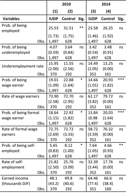
Table 1. Employment impact indicators, descriptive statistics
2010 2014
(1) (2) (3) (4) Variables IUDP Control Sig. IUDP Control Sig.
Prob. of being employed 25.53 31.51 ** 23.58 26.25 ns (1.73) (1.75) (1.46) (1.92) Obs. 1,497 628 1,497 628 Prob. of being underemployed 4.07 3.64 ns 3.42 3.48 ns (0.59) (0.84) (0.54) (0.91) Obs. 1,497 628 1,497 628 Underemployment rate 15.95 11.55 ns 14.49 13.25 ns (2.00) (2.56) (2.05) (0.00) Obs. 370 192 352 161 Prob. of being 19.01 22.88 * 14.66 20.93 *** wage earner (1.09) (1.64) (1.01) (1.82) Obs. 1,497 628 1,497 628 Rate of wage earners 73.90 72.70 ns 62.17 79.72 ns (2.58) (2.95) (3.82) (0.00)
Obs. 370 192 352 161 Prob. of being formal
wage earner
18.64 22.92 * 13.84 20.03 *** (1.15) (1.82) (0.98 (1.64) Obs. 1,497 628 1,497 628 Rate of formal wage
earners
72.75 72.72 ns 58.72 76.32 ns (2.69) (3.33) (3.59) (0.00) Obs. 370 192 352 161 Prob. of being
self-employed 5.65 8.12 * 7.64 4.66 ** (0.83) (1.00) (1.05) (0.93) Obs. 1,497 628 1,497 628 Rate of self-employment 21.82 25.76 ns 32.39 17.76 ns (2.50) (3.09) (3.44) (0.00) Obs. 370 192 352 161 Earned income (thousands DJF) 48.1 49.8 ns 64.46 66.6 ns (43.2) (40.6) (77.4) (38.4) Obs. 370 192 351 160 Note: Standard deviations in brackets. *** p<0.01, ** p<0.05, * p<0.1, ns: not significant.
The probabilities are calculated for the entire population aged 15 and over, whereas the rates concern the reference population. The “Sig.” columns test the significance of the difference between the previous two columns.
Source: 2010 & 2014 IUDP surveys, balanced individual panel. Authors’ calculations.
In 2010, the area has a strikingly small share of gainfully employed workers, accounting for just 25.5% of the labour force (cf. column (1) Table 1). More than a quarter (27%) of the households in the area do not have a single household member with a paid job. The share of individuals outside the labour force is remarkably high: half of all adults and 83% of young
15
people are inactive. This phenomenon affects women more than men.5Among employed workers, 15.9% are underemployed. Most of those who are employed are wage earners (73.9%), working in a small range of occupations and in the formal sector (72.8%) (cf. column (1) Table 1).6 Contrary to what can generally be observed in other developing countries, informal employment, defined as self-employment, is very low, with just 21.8% of workers considered as informal. These figures highlight the challenge facing policymakers to provide Balbala’s inhabitants with access to jobs and to develop productive activities in the district.
3. Methodology
The impact evaluation method uses a difference-in-difference approach. This method is valid when the observed trend differences between the control group and the treatment group are due solely to the impact of the IUDP. The equation estimated therefore takes the following form for the impact indicators measured at the individual level:
𝑦𝑖,𝑗,𝑔,𝑡 = 𝛼 + 𝛽𝑇 ∗ 𝐷2014+ 𝜂𝑇 + 𝜗𝐷2014+ 𝛾𝑋𝑗,𝑡+ 𝜖𝑖,𝑗,𝑔,𝑡 (1)
where 𝑦𝑖,𝑗,𝑔,𝑡 is an impact variable for individual i in household j living on block g in t
(𝑡 = 2010, 2014) and 𝜖𝑖,𝑗,𝑔,𝑡 is an idiosyncratic error term at the individual level. T is a
dummy variable that takes the value 1 when the individual lives in the IUDP zone and 0 otherwise. 𝐷2014 is a dummy variable that takes the value 1 for 2014 and 0 for 2010. Project
impact is captured by the interaction between variable T and time dummy variable 𝐷2014.
The coefficient of interest is therefore 𝛽 and represents the average impact of the IUDP. Vector 𝑋𝑗,𝑡 comprises variables that can vary over time. It includes the gender of the household head, variables capturing the household’s demographic composition (number of
5
The inactivity rate stands at 58% for women compared with 38% for men.
6
Women are mostly saleswomen (39%) and domestic servants (28%), while men are mainly in the armed forces (13%), security guards (11%), drivers (11%), refuse collectors (8%), and construction workers (5%).
16
male and female adults aged 25 to 49 and number of young people aged 15 to 24), and the highest level of education within the household. The descriptive statistics of the control variables are presented in Table A1 of the Appendix.
To control for potential differences in neighbourhood, household, and individual characteristics, we include individual fixed effects in the model. This specification is the first estimator implemented. Equation (1) is then written:
𝑦𝑖,𝑗,𝑔,𝑡= 𝛼 + 𝛽𝑇 ∗ 𝐷2014+ 𝜇 𝑖+ 𝜗𝐷2014+ 𝛾𝑋1𝑋
𝑗,𝑡+ 𝜖𝑖,𝑗,𝑔,𝑡 (2)
where 𝜇 𝑖 is a dummy variable at the individual level. Collinearity with treatment variable T means that this variable no longer appears in the equations.
Even if the control group had been chosen to have similar housing conditions and disconnection characteristics to the IUDP zone, Table 1 shows that the proportion of employed workers was higher in the control zone in 2010 than in the IUDP zone. Differences between the two neighbourhoods could well skew the impact evaluation insofar as they reflect different trends. Yet, we examine parallel trends by testing whether the two zones followed similar paths prior to the project launch (between 2007 and 2010). The results of the parallel trend test are presented in Table A2 (Appendix) and cannot reject the null hypothesis of parallel trends for all the indicators tested, except wage earners (the coefficient is however significant only at 10%). This test confirms the validity of the selection of the control group and the difference-in-difference method. However, the results on wage earners should be taken with caution.
To better control for a potential bias due to time-variant unobservables, we use the semi-parametric difference-in-difference estimator (Abadie, 2005). This estimator matches the IUDP zone individuals with the control zone individuals on the probability of being in the IUDP zone, 𝜋(𝑋2) ≡ ℙ(𝑑𝑡 = 1 |𝑋2), where 𝑋2 is a vector of observable characteristics at
17
the household level in 2010. In the case where 𝜋(𝑋2) < 1 and where ℙ(𝑑𝑡> 0), the
following sample 𝔼 (ℙ(𝑑∆𝑦𝑡 𝑡=1)𝑥
𝑑𝑡−𝜋(𝑋2)
1−𝜋(𝑋2)) gives an unbiased estimator of the average impact of the project. The estimator is a weighted average of the variation between 2010 and 2014, ∆𝑦𝑡 of variable 𝑦, with the households in the control group weighted by their probability of
being in the IUDP zone. Vector 𝑋2 comprises the following variables measured in 2010: gender, marital status, status in employment, level of education, speaking French or English, number of years lived in the household’s neighbourhood, household size, level of disconnection within the neighbourhood, and household’s standard of living measured by a standard-of-living score.7
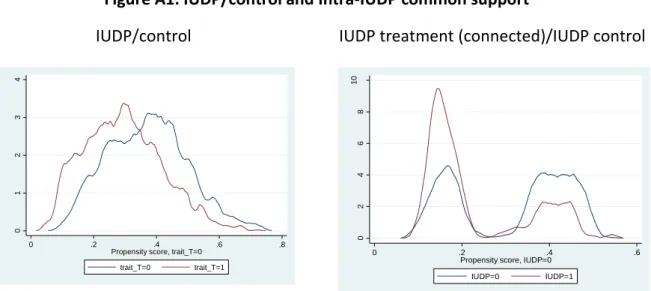
The estimations are restricted to a sample verifying the common support condition by dropping the treatment observations whose propensity score is higher than the maximum pscore for the controls or lower than the minimum pscore for the treatment (see graphs in the Appendix), and standard errors are calculated using the Abadie method (2005).
Another source of potential bias, attrition, is examined closely. First, we implement the Heckman (1979) selection model. The chosen exclusion variable is the desire expressed in 2010 to move out of the neighbourhood if possible, which is an important predictor of attrition (Table A3 in the Appendix). Second, we employ the nonparametric method following Lee (2009) that estimates explicit lower and upper treatment effect bounds in the presence of non-random sample attrition. This approach relies on two assumptions: the random assignment of treatment and monotonicity in the effect of treatment on attrition. This means that attrition should be lower in the treatment group than in the control group,
7 This standard-of-living score is calculated by multiple-component analysis using the following variables:
ownership of durable goods, frequency of consumption of fruit, vegetables, fish, and meat, level of household amenities (running water, electricity, and availability of a private toilet), and number of rooms in the dwelling occupied.
18
since people should be less eager to move out of the improved zone. It rests on a trimming procedure so that the share of observations with an observed outcome is equal for the treated and control groups. The lower and upper bounds of the treatment effect are computed (in the group that suffers less from attrition, either the largest or the smallest values of the outcome are regarded as ‘excess observations’ and are excluded from the analysis).
Given the fact that the individuals were not exposed to the treatment with the same intensity, the heterogeneity of the treatment method is also applied to obtain a body of evidence and capture the impact of the project through the extent of project exposure.
To address the potentially heterogeneous impact of the project, we identify different groups of individuals depending on the intensity of their exposure to the project components. Here again, the impact estimation follows the difference-in-difference principle. Yet unlike the previous approach, the control group and the treatment group are within the IUDP zone. Bear in mind that: (i) the neighbourhood’s connectivity is the central outcome of the IUDP in all the causality chains linking the outputs of the project to the targeted impacts on employment, and (ii) facilities such as public lighting, electricity, and water supply were installed alongside the new roadways. With these two key elements in mind, we identify the treatment group, which is made up of the individuals who benefitted from access to the new road network. Hence, the IUDP zone individuals are separated into two groups: the treatment group made up of the individuals “connected” as a result of the IUDP; and the control group comprising the individuals who have remained “disconnected,” and those who already lived in households close to roads before the project and consequently had no reason to change their way of life following the construction of the new roadways. The threshold to define “being connected as a result of the IUDP” is living less than 150 meters
19
from the new roads (represented by red points in map 1). We add distance to the health centre, community centre, and police station to the control variable vector in order to control for the potentially heterogeneous impact of these amenities on employment outcomes.8 The causal impact could potentially be difficult to assess due to the endogenous placement of the new roads. However, by implementing estimators with fixed effects and matching estimators, we control for both the economic and political characteristics that could drive the placement of the new roads. Moreover, the parallel trend test in Table A2 in the Appendix cannot reject the null hypothesis for all the indicators, confirming the validity of our method whatever the outcomes. Finally, we examine whether the results on the heterogeneous impact are robust to a potential attrition bias.
4. Results
Let us first analyse the overall impact of the IUDP project when individuals in the IUDP zone are compared with individuals in the control zone. The descriptive statistics of the outcome variables for the treatment group and the control group are shown in columns (1) to (4) of Table 1, while the diff-in-diff estimators are presented in columns (1) to (3) of Table 2. It can first be observed that the IUDP neighbourhood saw no improvement in access to employment from 2010 to 2014. The proportion of employed workers even dropped slightly over the period from 25.5% in 2010 to 23.6% in 2014 (Table 1). Looking at the estimations of the employment indicators in Table 2, no significant treatment impact is found on the employment rate, except for the one using the Heckman method with fixed effects. However, the Lee bounds on this outcome are -0.26 and 0.60 (not reported in the
8
The results remain unchanged when considering the continuous distance to the main road as an alternative specification (results not shown but available from the authors).
20
table); thus, the results appear not to be robust to a potential attrition bias.9 We can conclude that the IUDP project did not contribute to improving the likelihood of being employed.
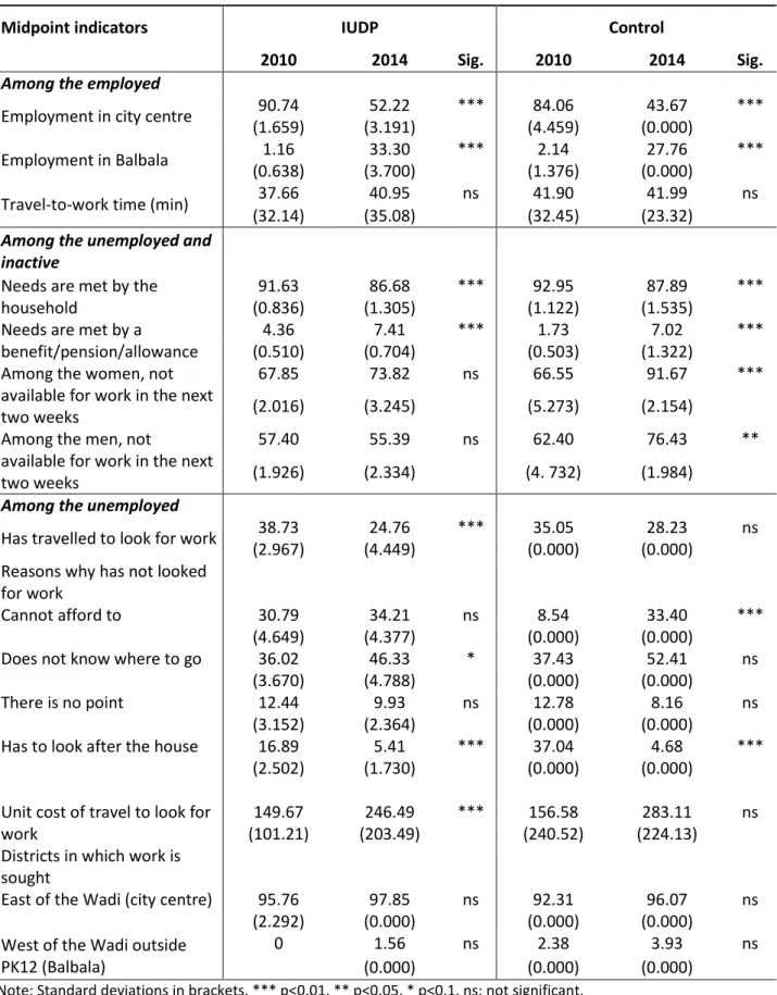
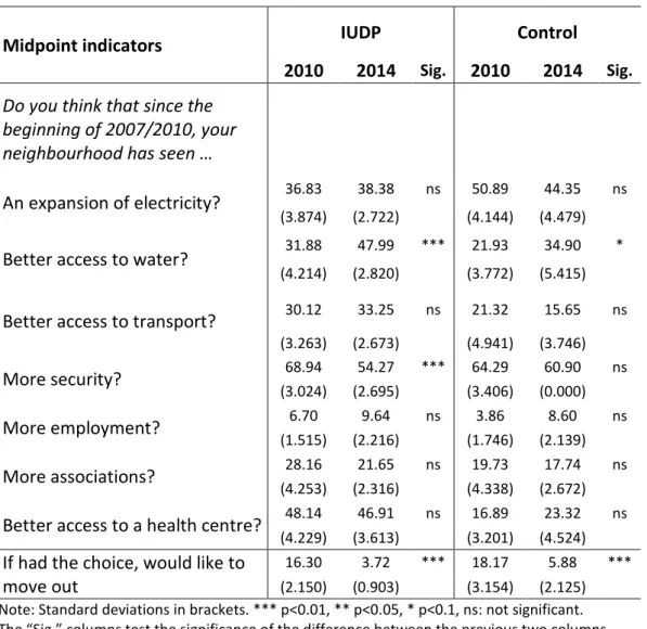
The effect of treatment on underemployment is non-significant in all the estimators (models [1] to [3]). This is hardly surprising given the small proportion of individuals who were underemployed in 2010: 16.0% of employed workers (Table 1) and 4.1% of individuals aged 15 and over. An analysis of the midpoint outputs of the project provides insight into why the IUDP project appears on average to have had no impact on employment variables (Table A5 in the Appendix). Bear in mind that the main channel is the reduction in job-seeking costs and more accessible information on vacancies due to the neighbourhoods’ improved connectivity. Yet job-seeking costs do not appear to have actually fallen. The unit cost for one trip to look for work shot up in the IUDP zone, virtually at the same rate as in the control zone. Consequently, the proportion of unemployed individuals travelling to look for work fell from 39% in 2010 to just 25% in 2014. If connecting the IUDP zone had no effect on the cost of travel to look for work, it is because job-seeking is conducted massively in the city centre (98% of cases in 2014 for the IUDP zone’s unemployed).10 The gains that could be made within the IUDP neighbourhoods are therefore marginal compared with the total cost of the trip. In addition, the main reason given by the discouraged unemployed to explain why they were not looking for work was not the cost of searching for a job, but not knowing where to look. Neither did improved connectivity bring individuals closer to the employment areas. The project did not reduce employed workers’ travel-to-work time. It remained stable, as in the control zone. More generally, individuals did not perceive any improvement in access to
9
Note that the monotonicity assumption seems not to be rejected, with the attrition rate equal to 46.0% in the control group and 40.5% in the treated group.
10
Djibouti City comprises two main areas, located on either side of the Ambouli Wadi: (i) the peninsula, where economic activity was initially concentrated, and (ii) the hills of Balbala, where the city has mostly spontaneously expanded since the 1970s.
21
transport in the neighbourhoods (Table A7 in the Appendix). Even if connecting the IUDP zone had reduced the cost of transport to access employment, the massive use of interpersonal networks11 to find work meant that this cost reduction would not necessarily have driven an increase in the employment rate in the zone.
The mismatch between the skills of the population in the IUDP zone and job vacancies could also explain the lack of impact of the IUDP on employment. In 2010, 70% of the unemployed had no work experience. Just 1% of the unemployed spoke English, a language often required to work in the foreign-owned ports and hotels that form the main employment areas.
Our finding tallies with the results found by Gonzalez-Navarro and Quintana-Domeque (2016) on the effect on employment of paving streets in Acayucan: paving did not significantly reduce travel-to-work cost and time.
However, these kinds of infrastructure projects could foster new local activities within the improved neighbourhoods. This effect is not evident from the average impact of the IUDP project. We find a positive and significant impact on the probability of holding a self-employed job for the Heckman estimator only (column (3), Table 2), and two negative impacts on the probability of being a wage earner or a wage earner in the formal sector for the matching estimator only (column (2), Table 2). When considering that those who left the IUDP zone before the end of the project could potentially have been impacted by this project (i.e. they are included in the treated group), the positive impact on the probability of holding a self-employed job is more robust. The coefficients are positive and significant in the three specifications (Table A4 in the Appendix). However, the lower Lee bound equals -0.06, so that the results appear not to be robust to a potential attrition bias.
11
22
The potential positive impact on self-employment corroborates the descriptive statistics in Table 1. The rate of self-employment increased by 10.6 percentage points, from 21.8% in 2010 to 32.4 % in 2014.
The IUDP therefore appears to have generated self-employment for the population benefitting from the project. Despite the small size of the sample of new self-employed workers, their characteristics can be outlined. Two-thirds were without work in 2010. Most of those in work in 2010 were men (77% of employed individuals in 2010) and wage earners in the city centre before becoming self-employed (73%). Most of those out of work in 2010 who were self-employed in 2014 were women (61%) working in a trade (61%) or service (25%), half of which were based in Balbala. The downturn in the proportion of wage earners among IUDP beneficiaries cannot be explained by individual transitions from wage employment to self-employment, as 78% of the wage earners in 2010 who were no longer in wage work in 2014 were no longer gainfully employed in 2014. In addition, most of those who were still in work were self-employed (60%) and working mainly in the city centre. The project had no effect on earned income. Real earned income may well have risen in the IUDP zone from 2010 to 2014, but the control zone also followed a similar trend.12
These initial results may conceal heterogeneous project effects, depending on the extent to which the investments financed by the project impacted the inhabitants of the IUDP zone. As already mentioned in the methodology section, those living closest to the main component of the project, i.e. the roads, could be expected to have benefitted more from the project. Columns (4) to (6) of Table 2 show the three estimators identified when the treatment group is composed of individuals who have been “connected” by the project, and when the control
12
However, when considering that those who left the IUDP zone before the end of the project were potentially impacted by this project (i.e. they are included in the treated group), the coefficients associated with earned income are positive and significant for specifications (1) and (3) (Table A4 in the Appendix).
23
group includes people who live in the IUDP zone, but whose distance from a road in 2014 was the same as in 2010. The descriptive statistics for the outcome variables of these two new treatment and control groups are shown in columns (1) and (2) of Table A5 in the Appendix. Broadly speaking, the same results as before are found for employment and underemployment. The individuals connected by the project compared with those whose distance from the road did not change experienced neither an increase in their probability of finding a job, nor a decrease in their underemployment.13
Yet the project seems to have significantly impacted self-employed activities. As can be seen in columns (4) to (6) of Table 2, the three estimators are all positive and significant in terms of the probability of being self-employed. Moreover, the Lee bound estimations show that this positive impact is robust to attrition bias, with the lower and upper bounds respectively equal to 0.03 and 0.05.14 We can thus consider the significantly positive effect of the project on the probability of working as a self-employed worker to be robust. This means that individuals have managed to develop local commercial activities or small-scale production in places adjacent to the project roads due to pavements that ease mobility within the zone and the setting up of informal activities. By contrast, the impact on the probability of being a wage earner is much less robust, as only one coefficient is negative and significant among the three estimators. Lastly, no significant impact is found on either the probability of being a formal wage earner or the real earned income of the new “connected” inhabitants.15 In a way, our results are close to those of Mu and van de Walle (2011) who find that the main effect of the rehabilitation of rural tracks in Vietnam is the development of activities
13
As suggested by one of the reviewers, we ran a robustness test by adjusting standard errors for spatial correlation; the coefficient associated with the unemployment variable becomes significantly negative.
14 This significant result compared to the non-significant bounds for the first specification comes from lower
attrition rates inside the IUDP of connected individuals (39.4%) and other inhabitants of the zone (46.4%).
15
However, when standard errors are adjusted for potential spatial correlation, the coefficients for wage earners and formal sector wage earners are significantly negative.
24
adjacent to the roads and the emergence of local markets with commercial activities. Similarly to Rand (2011) in Nicaragua, we observe that the individuals moving out of unemployment are women that predominantly achieve this through self-employment. On the other hand, and contrary to the effects of rural road projects in Georgia (Lokshin and Yemtsov, 2005), Bangladesh (Khandker et al., 2009), or Nicaragua (Rand, 2011), the IUDP project had no effect on transport time or costs; consequently, we observe no effect on formal jobs outside the neighbourhood. This can also be explained by Djibouti's unfavourable economic context, as the job supply is fairly limited. Both the lack of effect on formal employment and the small scale of the impact on informal activities in the neighbourhood explain the lack of effect of the IUDP project on living standards. This result is similar to that of Asher and Novosad (2020) in the case of rural India. Roads can only have a significant effect on poverty if the people targeted do not suffer from other constraints that prevent them from developing their own activities or finding wage employment.
25 Table 2. Employment impact indicator estimations
Employment impact indicators
Difference-in-difference with the control zone
Heterogeneity of treatment (difference-in-difference between
“connected” in 2014 versus same distance from road as in 2010 within
the IUDP zone)
(1) (2) (3) (4) (5) (6) Individual fixed effects (a) Matching (b) Heckman with fixed effects (a)
Individual fixed effects(c) Matching(b) Heckman with fixed effects (c) Employed 0.007 -0.014 0.043* -0.001 0.008 0.006 (0.029) (0.019) (0.025) (0.030) (0.026) (0.029) Underemployed 0.014 -0.010 -0.008 -0.016 -0.006 -0.011 (0.024) (0.012) (0.013) (0.018) (0.016) (0.016) Wage earners -0.020 -0.028* -0.004 -0.039 -0.041* -0.034 (0.023) (0.017) (0.020) (0.025) (0.021) (0.024)
Formal sector wage
earners -0.028 -0.036** -0.020 -0.027 -0.026 -0.020 (0.024) (0.017) (0.019) (0.025) (0.021) (0.025) Self-employed 0.035 0.012 0.046*** 0.035* 0.049** 0.037* (0.023) (0.013) (0.016) (0.020) (0.019) (0.019) Earned income (log) 0.375 -0.091 0.579 -0.057 -0.119 -0.044 (0.396) (0.273) (0.370) (0.454) (0.388) (0.436) Observations (individuals) 2,125 2,101 2,125 1,460 1,440 1,460
Note: population: individuals aged 15 years and over. Robust standard errors in brackets, clustered at the block level. * p<0.10, ** p<0.05,*** p<0.01.(a) The vector of control variables includes the household head’s gender and three variables capturing the household’s demographic composition – the number of adult men and women aged 25 to 49, the number of young people aged 15 to 24, and the highest level of education within the household.
(b) The propensity score is obtained based on the following variables measured in 2010: gender, marital status, status in employment, speaking French or English, level of education, number of years of residence in the neighbourhood, household size, a standard-of-living score measured by ownership of durable goods, frequency of consumption of fruit, vegetables, fish, and meat, level of household amenities (water supply, electricity, and availability of a private toilet), number of rooms in the dwelling occupied, and extent of disconnection. The estimations are restricted to a sample verifying the common support condition by dropping the treatment observations whose propensity score is higher than the maximum pscore for the controls or lower than the minimum pscore for the treatment, and standard errors are calculated using the Abadie method (2005). Consequently, 16 (9) treatment observations of the 2,101 (1,440) individuals for whom 2010 variables were available were dropped from the average (heterogeneous) estimation (col. 2 and col 5, respectively).
(c) The vector of control variables includes the household head’s gender and three variables capturing the household’s demographic composition – the number of adult men and women aged 25 to 49, the number of young people aged 15 to 24, the highest level of education within the household, and the distance to public amenities (health centre, community centre, and police station).
26 Conclusion
The purpose of this study was to evaluate the impact of an integrated urban upgrading project conducted in a slum in Djibouti City. The originality of the project lay in its combination of infrastructure construction and improvement to electrical and water supply facilities along the roads built. The method adopted consists in a difference-in-difference comparison of the IUDP zone with a control zone. We also examine the heterogeneity impact inside the IUDP zone, depending on project intensity through household distance from the roads.
The IUDP does appear to have stimulated microenterprise within the neighbourhoods by fostering the development of self-employment, in trade in particular. The main beneficiaries of this growth in self-employment were women who were outside the labour force before the IUDP. Yet there were not enough of these job creations to offset the downturn in wage employment in the zone and thereby improve access to employment. Indeed, the integrated upgrading project had no effect on individuals’ employment levels, as measured by the probability of being employed or underemployed. Neither did it improve their earnings. In time, the creation of self-employed activities may grow in the zone and reduce the unemployment and inactivity rates in the medium run. Nevertheless, since connectivity did not significantly reduce travel-to-work times, the project is unlikely to improve access to formal wage employment, as was expected at its outset.
While there is no denying that building infrastructures and roads in a neighbourhood improves the inhabitants’ quality of life and desire to stay there, our paper comes to a similar conclusion to Jaitman and Brakarz (2013) as to the absence of a significant impact of infrastructure upgrading programmes on employment and earnings. Although further evidence needs to be collected in order to draw a general conclusion as to the impact of
27
slum infrastructure upgrading programmes on employment, some observations can be made regarding these kinds of programmes. First, if all the channels are to be efficient, new infrastructures must allow for a reduction in the job-seeking cost and better access to information on vacancies. New roads are not sufficient to meet these objectives in contexts where interpersonal networks are used massively to get information on jobs and where transport is not or only slightly subsidized. As shown by Abebe et al. (2018) in Addis Ababa, transport subsidies coupled with job application workshops can change the spatial patterns of job search and employment. Second, whereas relocation programs are said to have fewer positive effects than in-situ upgrading programmes, we show that such upgrading programmes cannot be an efficient alternative if they are not associated with efficient social interventions. Improving connectivity with employment areas is not enough when the employability of slum inhabitants is very low. Although integrated programmes usually provide such interventions, they are generally undersized and poorly managed, as in the IUDP case. This paper calls for the implementation and evaluation of integrated infrastructure programmes including large social components.
Third, as advocated by van de Walle (2002), our results on the development of small activities, especially for poor women, argue for a better understanding of the distributive effects of these rehabilitation programmes. Looking back, this study can also hopefully contribute to drawing some lessons in terms of implementation and methodology for such impact evaluations.
28 References
Abadie A. (2005), “Semiparametric Difference-in-Differences Estimators”, Review of Economic Studies, 72(1): 1 – 19.
Abebe G. T., S. Caria, M. Fafchamps, P. Falco, S. Franklin and S. Quinn (2018), “Anonymity or Distance? Job Search and Labour Market Exclusion in a Growing African City”, Spatial Economic Research Centre, Discussion paper 224, 98p.
Asher S. and P. Novosad (2020) "Rural Roads and Local Economic Development." American Economic Review, 110 (3): 797-823.
Atuesta L. H. and Y. Soares (2018), “Urban upgrading in Rio de Janeiro: Evidence from the Favela-Bairro programme”, Urban Studies 55(1): 53-70.
Banerjee A., E. Duflo, R. Glennerster and C. Kinnan (2015), "The Miracle of Microfinance? Evidence from a Randomized Evaluation" American Economic Journal: Applied Economics, 7 (1): 22-53.
Clerc V., L. Criqui and G. Josse (2017), “Urbanisation autonome : pour une autre action urbaine sur les quartiers précaires“, Métropolitiques, Décembre, 7p.
Deboulet A. (2016), “Repenser les quartiers précaires“, Agence Française de Développement, collection Etudes n°13, 276p.
DISED (2012), Profil de la pauvreté en République de Djibouti, septembre, 43 p.
DISED (2018), Résultats de la quatrième enquête djiboutienne auprès des ménages pour les indicateurs sociaux (EDAM4-IS), Juin, 34 p.
Gonzalez-Navarro M. and C. Quintana-Domeque (2016), “Paving Streets for the Poor: Experimental Analysis of Infrastructure Effects”, The Review of Economics and Statistics, 98(2): 254-267.
Heckman J. (1979), “Sample Selection Bias as a Specification Error”, Econometrica, 47: 153-16.
Jaitman L. (2015), “Urban infrastructure in Latin America and the Caribbean: public policy priorities”, Latin American Economic Review, 24(1), 13.
Jaitman L. and J. Brakarz (2013), “Evaluation of slum upgrading programs, literature review and methodological approaches”, Inter-Americans Development Bank, Institutions for Development Sector technical note n° IDB-TN-604, November, 78 p.
Khandker S., Z. Bakht, and G. Koolwal (2009), “The poverty impact of rural roads: evidence from Bangladesh”, Economic development and cultural change, 57 (4), 685-722.
Lokshin M., and R. Yemtsov (2005), “Has rural infrastructure rehabilitation in Georgia helped the poor?” World Bank economic review, 19 (2), 311-333.
Lee D. S. (2009), “Training, Wages, and Sample Selection: Estimating Sharp Bounds on Treatment Effects”, Review of Economic Studies, 76(3): 1071–1102.
Marx B., T. Stoker and T. Suri (2013), “The Economics of Slums in the Developing World”, The
Journal of Economic Perspectives 27(4): 187-210.
Mu R. and D. van de Walle (2011), "Rural Roads and Local Market Development in Vietnam", Journal of Development Studies 47, 709-734.
29
Rand J. (2011) “Evaluating the employment-generating impact of rural roads in Nicaragua”, Journal of Development Effectiveness, 3(1): 28-43.
UN-Habitat (2013), Planning and Design for Sustainable Urban Mobility Global Report on Human Settlements 2013, United Nations Human Settlements Programme, Routledge, 317 p. van de Walle D. (2002), “Choosing Rural Road Investments to Help Reduce Poverty”, World Development, 30(4): 575–589.
Appendix
Descriptive statistics of control variables
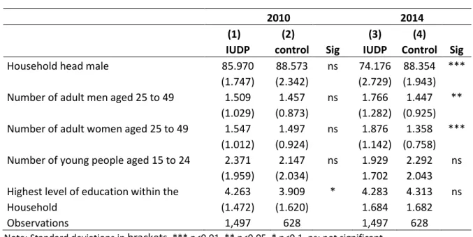
Table A1. Descriptive statistics, control variable
2010 2014
(1) (2) (3) (4)
IUDP control Sig IUDP Control Sig
Household head male 85.970 88.573 ns 74.176 88.354 ***
(1.747) (2.342) (2.729) (1.943)
Number of adult men aged 25 to 49 1.509 1.457 ns 1.766 1.447 **
(1.029) (0.873) (1.282) (0.925) Number of adult women aged 25 to 49 1.547 1.497 ns 1.876 1.358 ***
(1.012) (0.924) (1.142) (0.758) Number of young people aged 15 to 24 2.371 2.147 ns 1.929 2.292 ns
(1.959) (2.034) 1.702 2.043
Highest level of education within the 4.263 3.909 * 4.283 4.313 ns
Household (1.472) (1.620) 1.684 1.682
Observations 1,497 628 1,497 628
Note: Standard deviations in brackets. *** p<0.01, ** p<0.05, * p<0.1, ns: not significant. The “Sig.” columns test the significance of the difference between the previous two columns.
Source: 2010 & 2014 IUDP surveys, balanced individual panel. Authors’ calculations.
Test of the parallel trend assumption
The survey protocol was designed to test the parallel trend assumption as far as possible. This was done by putting retrospective questions to the individuals interviewed in 2010 about their situation three years before, in 2007. This was a placebo test to check whether living in the IUDP zone in 2010 made the indicators evolve differently between 2007 and 2010 from those for the inhabitants of the control zone. The tested assumption holds if this difference is not significant. These retrospective questions concerned the employment
30
status of the individuals aged 15 and over. Memory biases should be limited because the questions were asked at the individual level and not at the household level, and because 2007 was a landmark year with the 30th Anniversary of Independence Day. The sequential ordering of the questions should help limit this bias as well. People employed in 2010 were asked whether they had the same job on the 30th Anniversary of Independence Day (June 2007). If not, we asked them three questions to characterize their job. For the unemployed in 2010, we asked them whether they were employed, unemployed, or out of the labour force on the 30th Anniversary of Independence Day. If they were employed, we asked them the same three questions as for the 2010 and 2014 jobs.
Column (1) of Table A2 presents the results for the 2010-2014 panel of individuals. The null hypothesis of parallel trends cannot be rejected for all the variables except wage earner; the coefficient is however significant only at 10% (see results in Table A2).
Column (2) of Table A2 also presents the results of the test of this assumption on the sample of individuals living in the IUDP zone. The parallel trend assumption holds for all the employment indicators.
Table A2. Test of parallel trends between the IUDP zone and the control zone and within the IUDP zone
Variables (1) IUDP/Control zone (2) Intra-IUDP IUDP treatment (connected)/IUDP control Employed -0.011 0.024 (0.033) (0.032) Wage earner -0.041* 0.034 (0.024) (0.024) Self-employed -0.016 0.012 (0.017) (0.015) Observations 2,125 1,460
Robust standard errors in brackets; *** p<0.01, ** p<0.05, * p<0.1. Source: IUDP survey, 2010.
31 Matching common support
Figure A1. IUDP/control and Intra-IUDP common support
IUDP/control IUDP treatment (connected)/IUDP control
Source: 2010 & 2014 IUDP surveys, balanced household panel. Authors’ calculations.
0 1 2 3 4 d e n si ty 0 .2 .4 .6 .8
Propensity score, trait_T=0 trait_T=0 trait_T=1 0 2 4 6 8 10 d e n si ty 0 .2 .4 .6
Propensity score, IUDP=0
32 Attrition
Table A3. Selection equation, first-stage Heckman model, 2010-2014
(1) (2)
Variables IUDP/Control Intra-IUDP
Would like to move (1 = yes) 0.601*** 0.512*** (0.0585) (0.0754) Male head of household 0.00145 0.0249
(0.0619) (0.0747) Number of adult men -0.0775*** -0.101***
(0.0221) (0.0254) Number of adult women -0.105*** -0.0538**
(0.0211) (0.0256) Number of young people -0.0158 0.0218
(0.0117) (0.0146) Highest level of education in the household (reference: no education) Primary incomplete 0.298** 0.353** (0.120) (0.165) Primary complete 0.231*** 0.365*** (0.0880) (0.109) Lower secondary 0.282*** 0.362*** (0.0702) (0.0889) Upper secondary 0.492*** 0.511*** (0.0720) (0.0918) Higher 0.273*** 0.299*** (0.0807) (0.0981) Treatment 0.105** 0.000233 (0.0448) (0.000356) Distance to the health centre,
community 0.211*** centre, police station (0.0561) Constant -0.354*** -0.525***
(0.0938) (0.129)
Lambda coefficients (Mills ratio)
Employed -0.089 -0.250**
Underemployed -0.027 -0.067
Wage earner -0.052 -0.217**
Self-employed -0.044 -0.027
Formal employment -0.030 -0.135
Earned income (log) -1.106 -2.653*
Observations 3,913 2,678
Robust standard errors in brackets. *** p<0.01, ** p<0.05, * p<0.1. Source: IUDP survey, 2010 and 2014.
33 Robustness test
Table A4: Employment impact indicator estimations when those that left before the end of the project are included in the “treated” category
Employment impact indicators
Difference-in-difference with the control zone
Heterogeneity of treatment (difference-in-difference between “connected” in 2014 versus same distance from road as
in 2010 within the IUDP zone) (1) (2) (3) (4) (5) (6) Individual fixed effects (a) Matching (b) Heckman with fixed effects (a) Individual fixed effects(c)
Matching(b) Heckman with fixed effects (c) Employed 0.046 -0.075 0.055** 0.000 0.023 0.024 (0.029) (0.331) (0.025) (0.030) (0.036) (0.034) Underemployed 0.003 -0.008 -0.003 -0.015 -0.006 -0.007 (0.015) (0.011) (0.013) (0.018) (0.017) (0.016) Wage earners -0.023 -0.106 0.001 -0.038 -0.034 -0.043 (0.025) (0.330) (0.019) (0.025) (0.022) (0.031) Formal sector wage earners -0.030 -0.122 -0.019 -0.026 -0.018 -0.024 (0.024) (0.330) (0.020) (0.025) (0.022) (0.029) Self-employed 0.068*** 0.028** 0.053*** 0.035* 0.058* 0.052*** (0.018) (0.012) (0.017) (0.020) (0.031) (0.020) Earned income (log) 0.997** -1.024 0.761** -0.045 0.080 0.284
(0.431) (5.417) (0.360) (0.445) (0.519) (0.516) Observations (individuals) 2125 2107 2125 1485 1492 1460
34
Impact indicator levels in the treatment and control groups
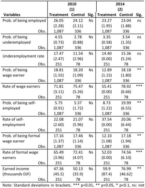
Table A5. Employment impact indicators intra-IUDP zone, 2010 - 2014
2010
(1)
2014 (2)
Variables Treatment Control Sig. Treatment Control Sig.
Prob. of being employed 26.05 24.12 Ns 23.27 23.04 ns (2.28) (2.11) (1.95) (1.88) Obs. 1,087 336 1,087 336 Prob. of being underemployed 4.55 2.78 Ns 3.35 3.54 ns (0.73) (0.88) (0.58) (1.35) Obs. 1,087 336 1,087 336 Underemployment rate 17.47 11.54 Ns 14.40 15.36 ns (2.47) (2.96) (0.00) (5.24) Obs. 251 78 251 78 Prob. of being 18.81 18.20 Ns 12.89 18.18 ** wage earner (1.55) (1.09) (1.15) (1.80) Obs. 1,087 336 1,087 336 Rate of wage earners 71.81 75.47 Ns 55.41 78.92 *** (3.11) (5.26) (0.00) (6.66)
Obs. 251 78 251 78 Prob. of being
self-employed 5.75 5.37 Ns 8.73 19.99 ** (0.91) (1.72) (1.22) (6.55) Obs. 1,087 336 1,087 336 Rate of self-employment 22.08 21.07 Ns 37.54 20.06 ** (2.60) (5.96) (0.00) (6.44) Obs. 251 78 251 78 Prob. of being formal
wage earner
17.16 17.46 Ns 12.10 17.18 ** (1.37) (1.14) (1.08) (1.94) Obs. 1,087 336 1,087 336 Rate of formal wage
earners 65.49 72.41 Ns 52.03 74.56 *** (3.96) (4.07) (0.00) (6.10) Obs. 251 78 251 78 Earned income (thousands DJF) 47.36 50.13 Ns 59.9 76.99 ** (45.5) (35.9) (87.4) (46.62) Obs. 251 78 251 78 Note: Standard deviations in brackets. *** p<0.01, ** p<0.05, * p<0.1, ns: not significant.
The probabilities are calculated for the entire population aged 15 and over, whereas the rates concern the reference population. The “Sig.” columns test the significance of the difference between the previous two columns.
Source: 2010 & 2014 IUDP surveys, balanced individual panel. Authors’ calculations.
35 Midpoint indicators
Table A6. Comparison of midpoint employment indicators between control zone and IUDP zone in 2010 and 2014
Midpoint indicators IUDP Control
2010 2014 Sig. 2010 2014 Sig.
Among the employed
Employment in city centre 90.74 52.22 *** 84.06 43.67 ***
(1.659) (3.191) (4.459) (0.000)
Employment in Balbala 1.16 33.30 *** 2.14 27.76 ***
(0.638) (3.700) (1.376) (0.000)
Travel-to-work time (min) 37.66 40.95 ns 41.90 41.99 ns
(32.14) (35.08) (32.45) (23.32)
Among the unemployed and
inactive
Needs are met by the household
91.63 86.68 *** 92.95 87.89 ***
(0.836) (1.305) (1.122) (1.535)
Needs are met by a
benefit/pension/allowance
4.36 7.41 *** 1.73 7.02 ***
(0.510) (0.704) (0.503) (1.322)
Among the women, not available for work in the next two weeks
67.85 73.82 ns 66.55 91.67 ***
(2.016) (3.245) (5.273) (2.154)
Among the men, not
available for work in the next two weeks
57.40 55.39 ns 62.40 76.43 **
(1.926) (2.334) (4. 732) (1.984)
Among the unemployed
Has travelled to look for work 38.73 24.76 *** 35.05 28.23 ns
(2.967) (4.449) (0.000) (0.000)
Reasons why has not looked
for work
Cannot afford to 30.79 34.21 ns 8.54 33.40 ***
(4.649) (4.377) (0.000) (0.000)
Does not know where to go 36.02 46.33 * 37.43 52.41 ns
(3.670) (4.788) (0.000) (0.000)
There is no point 12.44 9.93 ns 12.78 8.16 ns
(3.152) (2.364) (0.000) (0.000)
Has to look after the house 16.89 5.41 *** 37.04 4.68 ***
(2.502) (1.730) (0.000) (0.000)
Unit cost of travel to look for work
149.67 246.49 *** 156.58 283.11 ns
(101.21) (203.49) (240.52) (224.13)
Districts in which work is
sought
East of the Wadi (city centre) 95.76 97.85 ns 92.31 96.07 ns
(2.292) (0.000) (0.000) (0.000)
West of the Wadi outside PK12 (Balbala)
0 1.56 ns 2.38 3.93 ns
(0.000) (0.000) (0.000)
Note: Standard deviations in brackets. *** p<0.01, ** p<0.05, * p<0.1, ns: not significant. The “Sig.” columns test the significance of the difference between the previous two columns.