HAL Id: hal-00733457
https://hal-upec-upem.archives-ouvertes.fr/hal-00733457
Submitted on 19 Sep 2012
HAL is a multi-disciplinary open access
archive for the deposit and dissemination of
sci-entific research documents, whether they are
pub-lished or not. The documents may come from
teaching and research institutions in France or
abroad, or from public or private research centers.
L’archive ouverte pluridisciplinaire HAL, est
destinée au dépôt et à la diffusion de documents
scientifiques de niveau recherche, publiés ou non,
émanant des établissements d’enseignement et de
recherche français ou étrangers, des laboratoires
publics ou privés.
Wavelet-based restoration methods: application to 3D
confocal microscopy images
Caroline Chaux, Laure Blanc-Féraud, Josiane Zerubia
To cite this version:
Caroline Chaux, Laure Blanc-Féraud, Josiane Zerubia. Wavelet-based restoration methods:
applica-tion to 3D confocal microscopy images. SPIE 2007 Wavelets XII, Aug 2007, San Diego, CA, United
States. pp.67010E, �10.1117/12.731438�. �hal-00733457�
Wavelet-based restoration methods: application to 3D
confocal microscopy images
Caroline Chaux
a, Laure Blanc-F´eraud
aand Josiane Zerubia
a aARIANA Project-team, INRIA/CNRS/UNSA
2004 Route des lucioles - BP93
06902 Sophia-Antipolis, France
email: fi[email protected]
Keywords: restoration, deconvolution, 3D images, confocal microscopy, Poisson noise, wavelets
ABSTRACT
We propose in this paper an iterative algorithm for 3D confocal microcopy image restoration. The image quality is limited by the diffraction-limited nature of the optical system which causes blur and the reduced amount of light detected by the photomultiplier leading to a noise having Poisson statistics. Wavelets have proved to be very effective in image processing and have gained much popularity. Indeed, they allow to denoise efficiently images by applying a thresholding on coefficients. Moreover, they are used in algorithms as a regularization term and seem to be well adapted to preserve textures and small objects. In this work, we propose a 3D iterative wavelet-based algorithm and make some comparisons with state-of-the-art methods for restoration.
1. INTRODUCTION
Confocal microscopy1 is a powerful tool allowing to get an accurate view of cellular physiology, thus explaining its growing use in biological specimen imaging. Biological image quality is limited by two factors: a blur due to microscope optics (modeled by the Point Spread Function (PSF) denoted here by h), even if it is limited in confocal microscopy with respect to widefield microscopy, and the detection which is done with low photon flow leading to Poisson statistics.
The Richardson-Lucy algorithm2, 3 is often used to restore images in case of Poisson noise because of its well fitting. A regularization term has also been added in order to stabilize the inversion. More recently, some authors proposed to use the wavelet transform4, 5 for biological image deconvolution. In the literature of Poisson noise, many people use a pre-processing like the Anscombe6 transform or the Fisz transform7 in order to stabilize the noise variance and to apply more usual methods8 (i.e. techniques developed for Gaussian noise).
In the biological context, different approaches have been introduced: deconvolution and denoising steps are often splitted and then applied consecutively.
The approach considered here combines, in a unique algorithm, denoising and deconvolution. In this paper we propose a deconvolution method based on a 3D wavelet decomposition and an iterative deconvolution algorithm operating on the wavelet coefficients. We then make a comparative study of the different approaches considered in the biological microscopy context. The organization of the paper is as follows: in Section 2, we present the relevant background in biological microscopy image restoration. Then we introduce wavelets in Section 3 and the proposed algorithm in Section 4. Finally, we will give comparative results in Section 5 both on simulated and real data.
2. BACKGROUND
2.1. Problem context
Image formation model The considered image formation model is the following:
i =P(o ∗ h) (1)
where i is the observed image, o the original one,P(.) stands for Poisson noise and ∗ denotes the 3D convolution. We work with 3D objects, both for the images and the PSF (Point Spread Function) which is constructed
following different models (physical PSF, Gaussian PSF...). Image restoration (including both denoising and deconvolution) consists in estimating the original image, thus obtaining ˆo, only knowing the observation i (we assume here that the PSF is known).
PSF model The PSF modelizes the microscope optics. We consider here an analytical form of the PSF described by:
h(x, y, z) =|AR(x, y)∗ ˆPλem(x, y, z)| 2.
| ˆPλex(x, y, z)|2 (2) The excitation (resp. emission) wavelength is λex (resp. λem).
ˆ
Pλis the 2D Fourier transform on x, y of the pupil function Pλ, given by9–11:
Pλ(u, v, z) = Πρ ³p
u2+ v2´.e2iπλ .W(u,v,z) (3)
Here the complex term W (u, v, z) = 12z (1− cos 2α) is the aberration phase derived from11 . ρ = N A 2λ is the lateral cut-off frequency, and N A = nosin α the numerical aperture which is related to the amount of light en-tering the microscope and the immersion medium refractive index no. The phase W depends only on the defect of focus. This theoretical model of the confocal PSF does not take into account geometrical (e.g. spherical) lens aberrations and refractive index induced diffraction.
Noise nature: Poisson statistics At the same time, we are confronted with Poisson noise. A way to face this problem and use more conventional processing (stabilizing the variance) consists in either:
• applying the Anscombe transform6. This transformation is defined as follows:
A(i(x, y, z)) = 2 r
i(x, y, z) +3
8. (4)
• applying the Fisz transform7 . This transformation is defined as follows: 1. Process a non normalized Haar transform.
2. Transform the detail coefficients dj,m(k) of level j, subband m and spatial position k as
dj,m(k) = (
dj,m(k)/√aj,m(k) if aj,m(k)#= 0 0 if aj,m(k) = 0 where aj,m denotes the approximation coefficients.
3. Reconstruct using the inverse non normalized Haar transform.
After such transformations, the noise can be asymptotically considered asN (0, 1).
Some authors12 make the assumptions of a mixture of Gaussian noise (with mean µ and variance σ2) and Poisson noiseP(.). They consider the following image formation model:
i = αP(o ∗ h) + N (µ, σ2) (5) where α > 0 and develop adapted methods for image restoration problem.
2.2. Richardson-Lucy based algorithms
Many approaches are based on the Richardson-Lucy (RL) algorithm2, 3 which is well adapted to Poisson noise. One iteration of this algorithm is given by:
on+1(x) = ½· i(x) (on∗ h) (x) ¸ ∗ h(−x) ¾ on(x) . (6)
Several regularizations, allowing to stabilize the inversion, have been proposed such as:
Tikhonov-Miller regularization13 on+1(x) = ½· i(x) (on∗ h) (x) ¸ ∗ h(−x) ¾ o n(x) 1 + 2λT M△on(x) . (7)
Total variation regularization14, 15 The algorithm (RL-TV) is thus yielding to:
on+1(x) = ½· i(x) (on∗ h) (x) ¸ ∗ h(−x) ¾ o n(x) 1 − λ div³∇on(x) |∆on(x)| ´ . (8)
2.3. Separation of the denoising and deconvolution steps
In the microscopy field, researchers often apply deconvolution and denoising steps consecutively, thus introducing some difficulties. We discuss in this part the advantages and drawbacks of the different approaches.
2.3.1. Denoising then deconvolution
denoising algorithm Deconvolution STEP 1 STEP 2 Preprocessing preprocessing Inverse Wavelet o ˆo
Figure 1.Scheme of Method 1.
The denoising step often corresponds to a wavelet coefficient thresholding using wavelets4, 5 or steerable pyramids16 . Concerning the deconvolution step, RL algorithm or a MAP (Maximum A Posteriori) method is often used. When Poisson noise is considered, pre-processing stage to stabilize the noise variance is applied previously on the data.
Several drawbacks can be pointed out : we wonder whether the PSF is modified during the denoising step (in16 they estimate it after denoising); but also, we are not sure of the noise nature after the denoising step. Wavelets have shown to be really efficient in denoising problems, which leads naturally to method 1.
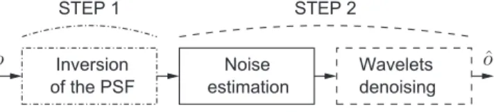
2.3.2. Deconvolution then denoising
Inversion of the PSF denoising Wavelets estimation Noise STEP 1 STEP 2 o oˆ
The deconvolution step often corresponds to an inversion of the PSF17taking into account it may have zeros. A simple way to achieve it is
F(ˆo) =
( F (o)
F (P SF ) if |F(P SF )| > ǫ
0 otherwise (9)
where F(.) denotes the Fourier transform. ǫ can be taken equal to 0.001.
Concerning the denoising step, it often corresponds to a coefficient thresholding in a transformed domain. The noise level has to be estimated. When Poisson noise is considered, pre-processing stage to stabilize the noise variance is previously applied on the data.
The approach creates an amplification of the noise during the deconvolution step and after the inversion of the PSF, the noise nature is not known. The second step (denoising) must take into account this particularity. This method is easy to implement and comes naturally to mind. Nevertheless, without an adaptation and a careful implementation,18 the noise is too strongly amplified and this method gives rise to bad results.
In order to tackle the different problems above mentioned, we propose to combine the denoising and decon-volution steps using a single algorithm operating in the 3D transformed domain, as we will see later.
3. 3D WAVELET ANALYSIS
This section aims at giving a brief recall of the 3D wavelet transform. We also propose here an anisotropic version of the transform.
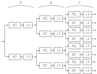
x y z H∗ 1 H∗ 1 ↓ 2 ↓ 2 H∗ 0 H∗ 1 ↓ 2 ↓ 2 H∗ 0 H∗ 0 ↓ 2 H∗ 1 ↓ 2 ↓ 2 H∗ 0 H∗ 1 ↓ 2 ↓ 2 H∗ 0 H∗ 1 ↓ 2 H∗ 0 ↓ 2 H∗ 1 ↓ 2 H∗ 0 ↓ 2 ↓ 2
Figure 3.Analysis filter bank for a 3D Discrete Wavelet Transform.
The classical 3D dyadic wavelet analysis of L2(R) involves one scaling function ψ
0 ∈ L2(R) and a mother wavelet ψ1∈ L2(R) such that:
∀m ∈ {0, 1}, √1 2ψm( t 2) = ∞ X k=−∞ hm[k]ψ0(t − k),
where (hm[k])k∈Z are real-valued square summable sequences. The analysis filter bank presented in Fig. 3 itered on the lowpass coefficients allows to realize the mutiresolution analysis.
Another specification of confocal microscopy is the difference of resolution in the z direction compared to the (x, y) directions. A way to tackle this problem would be to consider an anisotropic decomposition. By anisotropic, we mean to make a different processing (i.e. better adapted) in the z direction. We propose here to use a different wavelet in the z direction (as the decomposition is separable) and also to consider a different resolution level (lower). This is equivalent in Fig. 3 to use different filters in the z direction compared to the x and y directions
and stop the multiresolution analysis earlier for the z direction.
The coefficients obtained after such an analysis will be processed as presented in the next section.
4. PROPOSED ALGORITHM
We study here an iterative 3D wavelet-based algorithm19–21 allowing to operate conjointly denoising and de-convolution in the wavelet transform domain, considering the 3D Discrete Wavelet Transform presented in the previous section. The objective is to:
minimize o∈H 1 2h ∗ o − i! 2+X k∈K φk("o | ek#). (10)
This criterion is composed of two terms: a data fidelity term and a regularization term (which penalizes each wavelet coefficients) where the regularization function φk can be chosen adaptively.
The algorithm reads:
on+1= on+ λn(proxγnφk< on+ γn(h ∗
(i − hon))|ek>−on) (11) where ek stands for an orthonormal basis and prox denotes the proximity operator. Some properties of this operator as well as the convergence property of this algorithm are given in21 .
For instance, we can choose:
φ= ω | . | (12)
or φ = ω | . |2 (13)
where ω is a fixed parameter and φ a fixed regularization function. When φ is defined by (12), then the corresponding proxφ is a soft thresholding with threshold ω. We take γ = 1.99 (step size) and λ = 1 (relaxation parameter) in the numerical experiments.
This algorithm is directly applied to the coefficients issued from a 3D wavelet transform. When Poisson noise is considered, we apply a pre-processing on the data (Anscombe or Fisz), because this algorithm has been developed for Gaussian noise.
5. COMPARATIVE RESULTS
5.1. Initial definitions
In order to evaluate the quality improvement, we propose to use the I-divergence measure. The I-divergence22 between two 3D images o and ˆois given by:
Io,ˆo= X ijk ½ oijk.ln · oijk ˆ oijk ¸ − (oijk− ˆoijk) ¾ (14)
5.2. Tested images
We propose here to proceed the tests on simulated, phantom and real data.
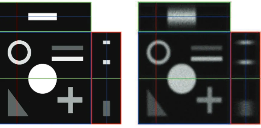
Synthetic image The first kind of data allows us to evaluate the proposed method performances in terms of qualitative but also quantitative measures. We suppose we know the original image and we add blur and noise in order to obtain the observed data. The original and degraded data are represented in Fig. 4.
We assume the microscope has a perfect pinhole and its characteristics are the following : • The magnification of the objective is 63×.
• The numerical aperture is 1.4 airy units.
• The excitation wavelength is 488nm whereas the emission wavelength is 520nm. • The voxel size is 0.02µm × 0.02µm × 0.05µm.
Figure 4.3D synthetic image. Original (left) and degraded (right).
Phantom image We consider here a spherical shell (as represented in Fig. 5) of diameter 15µm and which thickness is known to lie between 0.5µm and 0.7µm.
The acquisition is made using a microscope having the following parameters:
• The magnification of the objective is 63×.
• The refractive index of the medium is 1.33 and of the immersion lens medium (oil) is 1.518. • The numerical aperture is 1.4 airy units.
• The excitation wavelength is 488nm whereas the emission wavelength is 520nm. • The voxel size is 89.26nm × 89.26nm × 232.75nm.
The 3D image consists in 128 stacks of size 256 × 256 and one xy slice of the obtained image is shown in Fig. 7 (left). The objective is, knowing the original object size, to recover it after restoration process.
15 µm
Real image We also work with real 3D confocal microscopy images.
We consider here an image which consists in 30 stacks representing a regenerating mammalian skin (see Fig. 6). The acquisition parameters are the following :
• Microscope Zeiss Axiovert 200
• The magnification of the objective is 40×.
• The refractive index of the medium is 1.33 and of the immersion lens medium (oil) is 1.518. • The numerical aperture is 1.3 airy units.
• The excitation wavelength is 488nm whereas the emission wavelength is 520nm. • The pinhole size is equal to 71µm
• The voxel size is 0.45µm × 0.45µm × 1µm.
Figure 6. 3D real image: regenerating mammalian skin. cUMR 6543 CNRS / Institute of Signaling, Developmental Biology and Cancer.
5.3. Tested methods
Method 1: 1. Pre-processing 2. Wavelet denoising 3. Inverse Pre-processing 4. RL algorithm Method 2: 1. PSF inversion 2. Noise estimation 3. Wavelet denoising Method 3: 1. Pre-processing 2. Deconvolution + denoising 3. Inverse Pre-processingOn the one hand, when the noise is estimated (for example, after the PSF inversion in method 2), we use the robust median estimator which leads to the estimated variance ˆσ of σ considering the first level detail wavelet coefficients d1,(2,2)23 :
ˆ σ= 1
0.6745median[|d1,(2,2,2)|]. (15) On the other hand, when the noise is Poisson, we apply the Anscombe transform (see Section 2) in order to stabilize its variance to 1.
5.4. Quantitative and qualitative results
Synthetic image We propose, first, to give some numerical results comparing the three proposed methods. These preliminary tests allow us to calibrate the parameters. We consider symlets wavelets of length 16. For method 1, Sureshrink24 thresholding is applied followed by the RL algorithm. For method 2, we invert the PSF as described by (9) with ǫ = 0.001, then make an estimation of the noise level (using the robust median estimator) and apply Sureshrink thresholding. Concerning method 3, φ = 0.15| . | and in the anisotropic case, we replace the z wavelet by the Haar wavelet. In all cases, we choose the Anscombe transform as pre-processing stage.
I-div Initial value Method 1 Method 2 Method 3 Method 3 anis
6.98 1.17 2.11 1.09 0.90
Table 1.Restoration results (I-divergence) considering Poisson noise on the synthetic image.
As predicted, method 2 does not lead to good numerical results because it has to be better adapted. The anisotropic form of the wavelet transform allows to improve the I-divergence. The first approach also allows to obtain good results.
Phantom image The objective here is to recover the initial shell dimension.
Figure 7.Restoration of the shell. Raw data (left), restored images using method 1 (center) and method 3 (right).
In Fig. 7, we represent the original data (left) the restored data using method 1 (center) and the restored data using method 3 (right). It seems that method 3 leads to a reduced thickness. Let’s have a look to the intensity profile represented in Fig. 8. The observed data gives approximately a thickness of 1.2µm whereas method 1 leads to 1µm and method 3 to 0.76µm. The two first measurements are too large and the third one is a little bit too large but it better approximates the reality which means that method 3 allows to better recover the initial shell size.
0 5 10 15 20 25 30 35 0 20 40 60 80 100 120 140 160 180 Original Method 1 Method 3
Figure 8.Intensity profile of the 3 xy images respresented in Fig.7. 1 pixel represents 89nm.
Real image Now, we are interested in 3D real image restoration. The obtained results can be judged and evaluated visually.
In Fig. 9, we have represented two slices of the 3D image shown in Fig. 6. The right column corresponds to the restored images; the first impression can be mitigated but a careful look to these images allows to notice some improvements. In the upper left corner, we can see in the stack, the vitelline membrane which is considered as noise and alveolus structures which correspond to the central cells. In the upper right corner we have the restored image: the vitelline membrane has been removed and some central cells are recovered from noise. In the lower right corner, we can distinguish some filaments in the image which correspond to epidermal cells. In the associated restored image, a part of the noise has been removed allowing to recover some central cells and to better see epidermal cells.
6. CONCLUSION AND PERSPECTIVES
We have presented, in this paper, different image restoration methods for 3D confocal microscopy images based on wavelets. More sophisticated analyses such as the Dual-tree Wavelet Transform25, 26 could improve these restoration results at a price of a low redundancy.
Concerning the presented methods, the hyperparameters have been fixed empirically until now. An objective would be to computed them adaptively27 . The main idea we want to follow in the future is to develop directly Poisson statistic adapted methods.
7. ACKNOWLEDGMENTS
The authors want to thank J.-C. Olivo-Marin and B. Zhang (Pasteur Institute, France), Z. Kam (Weizmann Institute, Israel) and Arie Feuer (Technion, Israel), P. Pankajakshan (INRIA Sophia-Antipolis, France) for several interesting discussions.
We would like to thank Pasteur Institute and Nice University (UMR 6543 CNRS / Institute of Signaling, Developmental Biology and Cancer) for providing us the spherical shell images and the mammalian regenerating skin images, respectively. This research was partly supported by the P2R Franco-Israeli Collaborative Program. The first author would like to thank INRIA for funding her Post-doc fellowship.
Figure 9. Restoration of the the regenerating mammalian skin image. UMR 6543 CNRS / Institute of Signaling,c Developmental Biology and Cancer. Original data (left column) and corresponding restored images using method 3 (right column) .
REFERENCES
1. J. Pawley, Handbook of Biological Confocal Microscopy, Plenum Press, New York, 2nd ed., 1996.
2. W. H. Richardson, “Bayesian-based iterative method of image restoration,” J. of Opt. Soc. of Am. 62, pp. 55–59, 1972.
3. L. B. Lucy, “An iterative technique for rectification of observed distributions,” The Astronomical Jour-nal 79(6), pp. 745–765, 1974.
4. B. Colicchio, E. Maalouf, O. Haeberl´e, and A. Dieterlen, “Wavelet filtering applied to 3D wide field fluores-cence microscopy deconvolution,” in Proceedings PSIP’07, (Mulhouse, France), Jan. 31 - Feb. 2 2007. 5. J. Boutet de Monvel, S. Le Calvez, and M. Ulfendahl, “Image Restoration for Confocal Microscopy:
Improv-ing the Limits of Deconvolution, with Application to the Visualization of the Mammalian HearImprov-ing Organ,” Biophysical Journal 80, pp. 2455–2470, May 2001.
6. F. J. Anscombe, “The transformation, of Poisson, binomial and negative-binomial data,” Biometrika 35, pp. 246–254, Dec. 1948.
7. M. Fisz, “The limiting distribution function of two independent random variables and its statistical appli-cation,” in Colloquium Mathematicum, 3, pp. 138–146, 1955.
8. P. Besbeas, I. De Feis, and T. Sapatinas, “A comparative simulation study of wavelet shrinkage estimators for poisson counts,” Internat. Statist. Rev. 72(2), pp. 209–237, 2004.
9. M. Born and E. Wolf, Principles of Optics, Cambridge University Press, 7th (expanded) ed., 1999.
10. A. FitzGerrel, E. Dowski, and W. T. Cathey, “Defocus transfer function for circularly symmetric pupils,” Applied Optics 36, pp. 5796–5804, Aug. 1997.
11. J. W. Goodman, Introduction to Fourier Optics, McGraw-Hill Book Company, 2nd ed., 1996.
12. B. Zhang, J. Fadili, J.-L. Starck, and J.-C. Olivo-Marin, “Multiscale variance-stabilizing transform for mixed-Poisson-Gaussian processes and its applications in bioimaging,” in Proc. Int. Conf. on Image Proc. (ICIP), Sept. 2007.
13. G. van Kempen and L. van Vliet, “The influence of the regularization parameter and the first estimate on the performance of Tikhonov regularized non-linear image restoration algorithms,” Journal of Microscopy 198, pp. 63–75, Apr. 2000.
14. N. Dey, L. Blanc-F´eraud, C. Zimmer, Z. Kam, J.-C. Olivo-Marin, and J. Zerubia, “A deconvolution method for confocal microscopy with total variation regularization,” in Proceedings of ISBI’2004, April 2004. 15. N. Dey, L. Blanc-F´eraud, C. Zimmer, Z. Kam, P. Roux, J. Olivo-Marin, and J. Zerubia,
“Richardson-Lucy algorithm with total variation regularization for 3D confocal microscope deconvolution,” Microscopy Research Technique 69, pp. 260–266, 2006.
16. F. Rooms, W. Philips, and D. S. Lidke, “Simultaneous degradation estimation and restoration of confocal images and performances evaluation by colocalization analysis,” Journal of microscopy 218, pp. 22–36, Apr. 2005.
17. J. G. McNally, T. Karpova, J. Cooper, and J.-A. Conchello, “Three-dimensional imaging by deconvolution microscopy,” Methods 19, pp. 373–385, Nov. 1999.
18. J. Kalifa, S. Mallat, and B. Roug´e, “Deconvolution by thresholding in mirror wavelets bases,” IEEE Trans. on Image Processing 12, pp. 446–457, Apr. 2003.
19. J. Bect, L. Blanc-F´eraud, G. Aubert, and A. Chambolle, “A l1-unified variational framework for image restoration,” in Proc. European Conference on Computer Vision (ECCV), T. Pajdla and J. Matas, eds., LNCS 3024, pp. 1–13, Springer, (Prague, Czech Republic), May 2004.
20. I. Daubechies, M. Defrise, and C. De Mol, “An iterative thresholding algorithm for linear inverse problems with a sparsity constraint,” Comm. Pure Applied Math. 57, pp. 1413–1457, 2004.
21. P. L. Combettes and V. R. Wajs, “Signal recovery by proximal forward-backward splitting,” SIAM Journal on Multiscale Modeling and Simulation 4, pp. 1168–1200, Nov. 2005.
22. I. Csisz´ar, “Why least squares and maximum entropy?,” The Annals of Statistics 19, pp. 2032–2066, 1991. 23. S. Mallat, A wavelet tour of signal processing, Academic Press, San Diego, USA, 1998.
24. J. I. M. Donoho, D. L., “Adapting to unknown smoothness via wavelet shrinkage,” J. of American Statist. Ass. 90, pp. 1200–1224, 1995.
25. N. Kingsbury, “The dual-tree complex wavelet transform : a new efficient tool for image restoration and enhancement,” Proc. of EUSIPCO, Rhodes, Greece , pp. 319–322, 1998.
26. C. Chaux, L. Duval, and J.-C. Pesquet, “Image analysis using a dual-tree M -band wavelet transform,” IEEE Trans. on Image Proc. 15, pp. 2397–2412, Aug. 2006.
27. A. Jalobeanu, L. Blanc-F´eraud, and J. Zerubia, “Hyperparameter estimation for satellite image restoration using a MCMC maximum likelihood method,” Pattern Recognition 35(2), p. 341352, 2002.