HAL Id: hal-02990263
https://hal.archives-ouvertes.fr/hal-02990263
Submitted on 30 Nov 2020
HAL is a multi-disciplinary open access
archive for the deposit and dissemination of
sci-entific research documents, whether they are
pub-lished or not. The documents may come from
teaching and research institutions in France or
abroad, or from public or private research centers.
L’archive ouverte pluridisciplinaire HAL, est
destinée au dépôt et à la diffusion de documents
scientifiques de niveau recherche, publiés ou non,
émanant des établissements d’enseignement et de
recherche français ou étrangers, des laboratoires
publics ou privés.
multivariate bias correction via analogue ranks
resampling
Mathieu Vrac, Soulivanh Thao
To cite this version:
Mathieu Vrac, Soulivanh Thao. R2D2: Accounting for temporal dependences in multivariate bias
correction via analogue ranks resampling. Geoscientific Model Development, European Geosciences
Union, 2020, 13, pp.5367 - 5387. �10.5194/gmd-13-5367-2020�. �hal-02990263�
https://doi.org/10.5194/gmd-13-5367-2020 © Author(s) 2020. This work is distributed under the Creative Commons Attribution 4.0 License.
R
2
D
2
v2.0: accounting for temporal dependences in multivariate
bias correction via analogue rank resampling
Mathieu Vrac and Soulivanh Thao
Laboratoire des Sciences du Climat et de l’Environnement (LSCE-IPSL), CEA/CNRS/UVSQ, Université Paris-Saclay Centre d’Etudes de Saclay, Orme des Merisiers, 91191 Gif-sur-Yvette, France
Correspondence: Mathieu Vrac ([email protected]) Received: 6 May 2020 – Discussion started: 30 June 2020
Revised: 14 September 2020 – Accepted: 23 September 2020 – Published: 6 November 2020
Abstract. Over the last few years, multivariate bias correc-tion methods have been developed to adjust spatial and/or inter-variable dependence properties of climate simulations. Most of them do not correct – and sometimes even degrade – the associated temporal features. Here, we propose a mul-tivariate method to adjust the spatial and/or inter-variable properties while also accounting for the temporal depen-dence, such as autocorrelations. Our method consists of an extension of a previously developed approach that relies on an analogue-based method applied to the ranks of the time series to be corrected rather than to their “raw” values. Sev-eral configurations are tested and compared on daily tem-perature and precipitation simulations over Europe from one Earth system model. Those differ by the conditioning in-formation used to compute the analogues and can include multiple variables at each given time, a univariate variable lagged over several time steps or both – multiple variables lagged over time steps. Compared to the initial approach, results of the multivariate corrections show that, while the spatial and inter-variable correlations are still satisfactorily corrected even when increasing the dimension of the con-ditioning, the temporal autocorrelations are improved with some of the tested configurations of this extension. A major result is also that the choice of the information to condition the analogues is key since it partially drives the capability of the proposed method to reconstruct proper multivariate de-pendences.
1 Introduction
Climate model simulations are and will remain the main source of numerical projections to understand and antici-pate climate change consequences. Those projections are performed under various greenhouse gas emission scenarios, prescribed for instance within the fifth international Coupled Model Intercomparison Project (CMIP5; IPCC, 2013) or the ongoing CMIP6 (Eyring et al., 2016) and are widely used by the scientific community investigating climate changes and their manifold impacts. Indeed, climate changes have been anticipated to affect multiple domains: hydrology and water resources (e.g., Gleick, 1989; Christensen et al., 2004; Piao et al., 2010), agronomy and crops (e.g., Ciais et al., 2005; Ben-Ari et al., 2018), ecology and biodiversity (e.g., Brown et al., 2011; Bellard et al., 2012), economy (e.g., OCDE, 2015; Tol, 2018) or human migrations (e.g., Defrance et al., 2017) are examples of domains where expected impacts of climate evolution can be high and therefore quite problem-atic for society.
To get robust impact estimations, the climate projections have thus to be as precise and informative as possible. How-ever, even simulations of the current climate often present statistical biases: their mean, variance or more generally their distributions can more or less largely differ from observa-tional reference datasets (see, e.g., Christensen et al., 2008; Teutschbein and Seibert, 2012; François et al., 2020, among many other studies). This also means that climate projections for future periods are also expected to have biases, poten-tially similar. That is why many impact studies, for current or future climate, have to rely on “adjusted” climate simu-lations obtained via bias correction (BC) methods. Over the
last decades, many statistical and data-science BC techniques have been progressively devised for this specific purpose. The objective of such techniques is to transform (i.e., “cor-rect” or “adjust”) the climate model simulations such that, for a calibration time period, the obtained corrections are equivalent to a reference dataset in terms of one or several targeted statistical features (e.g., means, variances or distri-butions). Simple methods can be used in the event that the target is only the mean (as the so-called “delta” or “anomaly” methods, e.g., Xu, 1999) or the variance (e.g., “simple scal-ing” Eden et al., 2012; Schmidli et al., 2006). Neverthe-less, in general, the most employed methods are based on the “quantile-mapping” approach (e.g., Déqué, 2007; Gud-mundsson et al., 2012) and its many variants (e.g., Kallache et al., 2011; Vrac et al., 2012; Cannon et al., 2015), whose target is the whole univariate distribution (i.e., not only the mean and variance but all moments of higher order, as well as any percentile) of a given climate variable.
However, if many statistical aspects can be adjusted with such methods, all are only univariate, i.e., related to only one physical variable at a single location. If multiple vari-ables and/or at multiple locations have to be corrected, the in-dependent applications of several one-dimensional bias cor-rection (1d-BC) methods will not modify the intrinsic de-pendence structure of the simulations to be corrected (Vrac, 2018). Therefore, if the climate model simulations have bi-ases in their inter-variable and/or inter-site dependences (e.g., in their correlations), most of the quantile-mapping and uni-variate BC techniques will not correct these features and will basically preserve their biases. This obviously has con-sequences for the impact models requiring multiple climate variables as input: if the physical relationships (i.e., the sta-tistical dependences) of those input variables are not real-istic enough, the biases in the multivariate situations can quickly propagate to the simulated impacts themselves, even if the simulations are adjusted by 1d-BC methods (e.g., Boé et al., 2007). More generally in climate sciences, the accurate modeling of dependences is a key aspect for proper assess-ments and projections of compound events and their asso-ciated risks (e.g., Leonard et al., 2014; Zscheischler et al., 2018; Bevacqua et al., 2019).
Consequently, some multivariate bias correction (MBC) methods have been recently designed to tackle the issues of the biases in multivariate dependences. The goal is basically the same as for univariate corrections: find a transformation that makes climate model simulations have the same targeted statistical features as a reference in the calibration period. In this case, the target statistical features include not only univariate features but also multivariate statistical features such as correlations or the empirical copula. The various MBCs developed so far can be categorized into three main families (Vrac, 2018; Robin et al., 2019; François et al., 2020):
– the “marginal/dependence” approaches, correcting sep-arately univariate distributions and dependences before joining them to provide multivariate corrections (e.g., Vrac, 2018; Cannon, 2017);
– the “conditional successive” methods, adjusting one variable at a time but conditionally on the previously corrected variables to ensure proper multidimensional relationships (e.g., Piani and Haerter, 2012; Dekens et al., 2017);
– the “all-in-one” models, which do not separate the mul-tivariate distribution, neither in marginal/dependence, nor in conditional distributions, but directly transform one multidimensional distribution into another multidi-mensional distribution (e.g., Robin et al., 2019). A first intercomparison and critical review of MBC meth-ods has been carried out by François et al. (2020). One ma-jor finding was that, although most of the MBC techniques (depending on their hypotheses and configurations) are more or less able to provide adjusted multidimensional properties, none of them explicitly account for temporal dependence properties. This implies that, although multivariate properties can be correctly adjusted (and sometimes, spatial properties as well, depending on the method), the temporal structure of the data generated by MBC methods is different from that of the model data to be corrected but not necessarily closer to that of the reference data. Therefore, there is a need to im-prove temporal properties resulting from MBC outputs. Of course, this specific need should not be filled at the expense of the other (marginal, inter-variable or inter-site) properties. In the present study, we rely on a recently developed MBC method named R2D2 to propose an extension allowing us to improve the autocorrelation of the multivariate adjusted data. This R2D2extension takes advantage of an analogue-based technique to reconstruct the multidimensional depen-dence conditionally on a temporal sequences of ranks.
The rest of this article is organized as follows: Sect. 2 de-scribes the reference and model data on which the proposed R2D2extension is evaluated. Section 3 provides a short re-minder about the initial R2D2approach and the detailed de-scription of its new extension, as well as the experimental design set up for evaluation. Then, results are given and ana-lyzed in Sect. 4, under the following underlying focus ques-tion: can the suggested method improve the temporal depen-dences without degrading the other (marginal, spatial and inter-variable) properties? Finally, the main findings are sum-marized and discussed in Sect. 5.
2 Reference and model data
To perform tests and analyses of the proposed correction method, we will rely on daily temperature at 2 m (T2) and precipitation (PR) from one run of a global climate model
to be corrected on one hand and from an observation-based reference dataset on the other hand.
The latter corresponds to WFDEI data, which are the WATCH Forcing Data (WFD; Weedon et al., 2011) method-ology applied to ERA-Interim data for the period from 1 Jan-uary 1979 to 31 December 2016 on a 0.5◦×0.5◦spatial grid (Weedon et al., 2014) over the land-only European region (30◦N, −10◦E – 70◦N, 30◦E), corresponding to 4167 grid points.
The climate model data to be corrected are extracted – for the same region – from simulations performed by the IPSL-CM5A-MR Earth system model (Marti et al., 2010; Dufresne et al., 2013). Historical simulations from the en-semble member “r1i1p1” are used for 1979–2005. This is concatenated with simulations under RCP8.5 scenario made from the same ensemble member for 2006–2016, hence pro-viding a 1979–2016 time period. Those simulations have an initial 1.25◦×2.5◦spatial resolution. To allow comparisons
and applications of BC methods, they are then regridded to the WFDEI spatial resolution with a bi-cubic interpolation for temperature and a conservative interpolation for precipi-tation.
Note that only one climate model is used for application and evaluation purposes in the present study. Of course, other models will have other biases that must be corrected differ-ently. However, our goal is not to test the proposed approach on many climate models but rather to establish a proof of concept of the R2D2extensions on an illustrative simulations run. We hypothesize that the main general findings obtained on this single model will still be valid for other models and simulations.
3 Methods and design of experiments 3.1 A short reminder about the R2D2method
The proposed methodology relies on – or can be seen as an extension of – the Rank Resampling for Distri-butions and Dependences (R2D2) bias correction method (Vrac, 2018). R2D2 consists of two steps: first, a univari-ate BC is performed to adjust the marginal distributions, and then the empirical copula function (i.e., the depen-dence structure between the variables of interest, rid of their marginal distribution) is adjusted. Thus, R2D2belongs to the “marginal/dependence” family of multivariate bias correc-tions (see François et al., 2020, for a description of the other families: “successive conditional” and “all in one”).
For the first step, any 1d-BC method can be employed. In Vrac (2018) and in the following details of the present study, the cumulative distribution function – transform (CDF-t) ap-proach, e.g., Vrac et al. (2012), is used to adjust the marginal properties for temperature. A specific version of CDF-t is used to correct precipitation data. This version relies on a stochastic singularity removal (SSR; Vrac et al., 2016)
ap-proach to manage dry time steps: first, zeros (from both ref-erences and simulations) are randomly transformed to pos-itive but very small values (< 10−6); then CDF-t is applied onto the whole set of data (i.e., transformed data and ini-tially positive values altogether), and the correction results are thresholded such that values < 10−6are set to 0.
For the second step, R2D2 uses a “conditioning dimen-sion” (called “reference variable” in Vrac, 2018) from the 1d-BC results. This univariate 1d-BC time series – and more precisely its ranks – serves as a conditioning to find, within the other 1d-BC variables, the values that have the same rank associations as those in the training reference dataset (details and examples on R2D2can be found in Vrac, 2018). Hence, this method relies on a univariate conditioning dimension to generate rank associations, in the same way as an analogue technique (initially developed by Lorenz, 1969) relies on its predictors to generate values. By doing so, this MBC ap-proach allows us to reproduce observed multivariate (spatial and multi-variable) dependence structures, while preserving some temporal properties of the initial simulations via the conditioning dimension.
However, if the temporal features of the conditioning di-mension (i.e., one physical variable at one given location) is preserved by construction, this is not necessarily the case for the other variables (i.e., different physical variables and/or spatial locations) and even not the case at all for variables having a weak rank correlations with the conditioning di-mension. Therefore, taking advantage of the analogue-based philosophy of R2D2, several extensions are here proposed to improve the temporal properties of the corrections brought by the initial R2D2.
3.2 Accounting for temporal structures via multivariate rank conditioning
The main idea of the proposed extensions consists of seeing the R2D2approach as an analogue-based method. Indeed, in Sect. 3.1, it is clear that the resampling of the multivariate ranks is conditional to a single rank value of the conditioning dimension. In analogue techniques used in the climate litera-ture (e.g., Zorita and von Storch, 1999; Yiou, 2014; Jézéquel et al., 2018, among others), the conditioning (i.e., predictor) variable can be multivariate. In our case, since the purpose of R2D2is to correct the dependence structure, we want the notion of analogue situations to only account for the depen-dence structure and not for the marginal distribution. Hence, the distance between two situations is not computed based on the raw values of the conditioning dimensions but based on their ranks. The best analogue is thus defined as the situation (e.g., day) having the association of ranks the closest to that of the conditioning dimension in terms of Euclidean distance. Here, an extension of R2D2is proposed and allows different configurations, all relying on R2D2applied conditionally on a multidimensional conditioning dimension:
– R2D2 conditional on a multivariate information at a
given time t . The conditioning dimensions in R2D2can be chosen freely. They can belong to the set of variables to be corrected, provided as exogenous variables or be a combination of both. There is no restriction either on the spatial scales of the conditioning dimensions. For in-stance, as a bivariate conditioning dimension, one could combine a daily North Atlantic Oscillation (NAO) in-dex, to provide large-scale information, with the tem-perature at one grid point as a source of small-scale information. Other choices could be the temperature at two given locations, the temperature and the precipita-tion at one locaprecipita-tion, etc.
– R2D2conditional on a rank sequence at times (t −n, t − n+1, . . ., t ) of a univariate conditioning dimension. The idea here is about the same as in the previous sugges-tion but instead of condisugges-tioning the rank resampling on a multivariate conditioning dimension at time t , it is on a univariate one (e.g., temperature at a given location, or NAO index) but at several (e.g., n) lagged time steps (t − n, t − n + 1, . . ., t ).
– R2D2conditional on a rank sequence of a multivariate conditioning dimension. This is a logical combination of the two previous configurations to condition R2D2 on information characterizing a temporal sequence of multiple variables.
Whatever the configuration, the choice of the conditioning dimension is however not trivial, as it conditions the tempo-ral properties of the model that will be conserved after cor-rection. In the case of a configuration accounting for the rank sequence, the length of the sequence to search the analogues has to be chosen. This length will be referred to as “Block-A” (for “block analogue”) hereafter. Moreover, in order to avoid discontinuities in the reconstructed final sequence of ranks, the whole sequence of the best analogue is not fully kept but only a subsequence corresponding to a given number of elements at the end of the complete sequence. This kept subsequence is referred to as “Block-K” (for “block kept”) hereafter, and its length also has to be chosen as shorter than or equal to Block-A. Searching for the best analogue with a length Block-A and then keeping only a length Block-K – shorter than Block-A – allows us to not only avoid disconti-nuities in the (rank and correction) time series but also give flexibility to the proposed BC method to adapt to the tem-poral dynamics of the climate model to correct. Preliminary tests (not shown) indicate that Block-A = 9 and Block-K = 7 are reasonable choices and that the results are only weakly influenced by a slight change of those values.
In the case of ties for the choice of best analogues, the proposed R2D2 algorithm selects the first time step having the minimal Euclidean distance. Hence, the order in which the dataset is searched to find the analogue ranks will in-fluence the selected time step and may thus potentially also
influence the results. For example, ties might occur when in-cluding daily precipitation as a conditioning variable, par-ticularly when precipitation at a single location is the only conditioning dimension. Indeed, there are potentially many time steps where it did not rain at the conditioning location. All of these time steps would all have the same rank (in this case, 1). This means that some rank combinations that are also compatible with the rank of the conditioning dimension (in this example, no rain at the conditioning location) will not be present in the corrected dataset. Hence, some rank asso-ciations can be either under-represented or over-represented in the corrected dataset compared to the reference dataset be-cause of ties in the conditioning dimensions. However, when using multiple conditioning dimensions (i.e., multiple condi-tioning locations and/or variables), the number of candidates for the best analogue with the same exact minimal Euclidean distance decreases, hence reducing the effect of the ties in the time series of the conditioning dimensions. Other choices could be made to deal with tied ranks: last or median time step (instead of first) could be selected or even a randomly drawn time step (among those with a common minimal dis-tance to the condition information). Nevertheless, this is not investigated in the present paper and left for future work.
In the following, 20 different R2D2configurations are ap-plied and compared to the reference WFDEI dataset, the plain simulations and the univariate BC results obtained from CDF-t. Those 20 configurations and their notations are given in Table 1. For the versions including five grid points in the conditioning, the locations are chosen to characterize five cities – Paris, Madrid, Stockholm, Rome and Warsaw – spread out over the region. In the same manner – but more automatically – the N grid points (N = 100 or 400) in the other versions are chosen to uniformly cover the region of interest.
Note that the configuration using a conditioning with only one physical variable at a single location without accounting for lags (i.e., R.1.1.0) exactly corresponds to the initial R2D2 method.
Moreover, in practice, the R2D2configurations with 400 grid points or with 4167 (i.e., all) grid points for the con-ditioning dimension provided results equivalent to those from the same configurations but with only 100 grid points (not shown). This emphasizes a preliminary result: taking a large number of spatial information is not necessarily needed once a sufficient information is provided. Hence, in the following, experiments R.400.1.0, R.400.2.0, R.400.1.1 and R.400.2.1 will not be presented, nor will experiments R.4167.1.0, R.4167.2.0, R.4167.1.1 and R.4167.2.1, as they provide results similar to R.100.1.0, R.100.2.0, R.100.1.1 and R.100.2.1, respectively.
3.3 Experimental design of the correction schemes The different configurations of the R2D2extensions, as well as the CDF-t univariate BC (referred to as BC1D in the
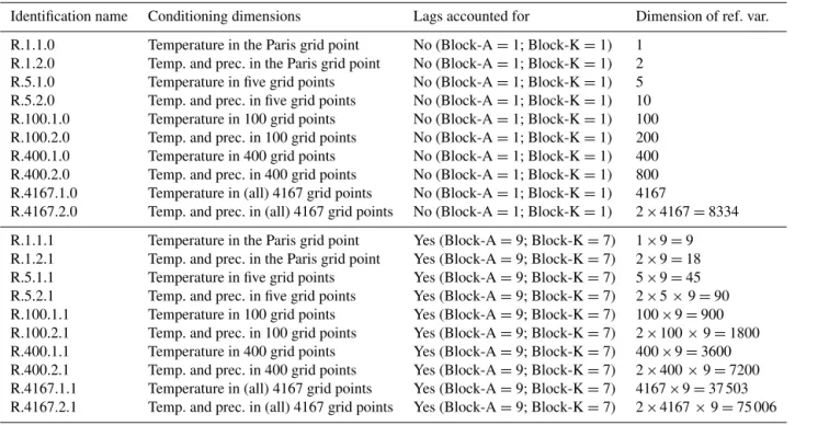
fol-Table 1. Summary of the 20 R2D2configurations tested. The identification name is organized in the following way. The first number indicates the number of grid points used for the conditioning dimension of R2D2; the second one corresponds to the number of variables considered at each grid point for the conditioning dimension (here, “1” indicates “only temperature”; “2” indicates “temperature and precipitation”); and the third number indicates if some lagged (i.e., temporal) information is used by R2D2(“0” means “no lag used”; “1” means “lags used”). “Block-A” corresponds to the block size (i.e., lag length) used for the analogue search and “Block-K” to the block size that is kept from the selected analogues of size Block-A.
Identification name Conditioning dimensions Lags accounted for Dimension of ref. var. R.1.1.0 Temperature in the Paris grid point No (Block-A = 1; Block-K = 1) 1
R.1.2.0 Temp. and prec. in the Paris grid point No (Block-A = 1; Block-K = 1) 2 R.5.1.0 Temperature in five grid points No (Block-A = 1; Block-K = 1) 5 R.5.2.0 Temp. and prec. in five grid points No (Block-A = 1; Block-K = 1) 10 R.100.1.0 Temperature in 100 grid points No (Block-A = 1; Block-K = 1) 100 R.100.2.0 Temp. and prec. in 100 grid points No (Block-A = 1; Block-K = 1) 200 R.400.1.0 Temperature in 400 grid points No (Block-A = 1; Block-K = 1) 400 R.400.2.0 Temp. and prec. in 400 grid points No (Block-A = 1; Block-K = 1) 800 R.4167.1.0 Temperature in (all) 4167 grid points No (Block-A = 1; Block-K = 1) 4167
R.4167.2.0 Temp. and prec. in (all) 4167 grid points No (Block-A = 1; Block-K = 1) 2 × 4167 = 8334 R.1.1.1 Temperature in the Paris grid point Yes (Block-A = 9; Block-K = 7) 1 × 9 = 9 R.1.2.1 Temp. and prec. in the Paris grid point Yes (Block-A = 9; Block-K = 7) 2 × 9 = 18 R.5.1.1 Temperature in five grid points Yes (Block-A = 9; Block-K = 7) 5 × 9 = 45 R.5.2.1 Temp. and prec. in five grid points Yes (Block-A = 9; Block-K = 7) 2 × 5 × 9 = 90 R.100.1.1 Temperature in 100 grid points Yes (Block-A = 9; Block-K = 7) 100 × 9 = 900 R.100.2.1 Temp. and prec. in 100 grid points Yes (Block-A = 9; Block-K = 7) 2 × 100 × 9 = 1800 R.400.1.1 Temperature in 400 grid points Yes (Block-A = 9; Block-K = 7) 400 × 9 = 3600 R.400.2.1 Temp. and prec. in 400 grid points Yes (Block-A = 9; Block-K = 7) 2 × 400 × 9 = 7200 R.4167.1.1 Temperature in (all) 4167 grid points Yes (Block-A = 9; Block-K = 7) 4167 × 9 = 37 503 R.4167.2.1 Temp. and prec. in (all) 4167 grid points Yes (Block-A = 9; Block-K = 7) 2 × 4167 × 9 = 75 006
lowing), are applied and evaluated according to the following 2-fold cross-validation approach. First, the methods are cali-brated over the 1979–1997 period and applied to correct the 1998–2016 climate projections for evaluation. Then, they are also applied the other way around, i.e., calibrated on 1998– 2016 and applied for evaluation on 1979–1997. Finally, the two 19-year evaluation periods are gathered to dispose of the whole 38-year time period for evaluation.
Every method is applied on daily values but on a monthly basis, i.e., for each month separately that are joined after-wards. However, evaluations are performed on a seasonal ba-sis – i.e., for each season (DJF, MAM, JJA, SON) separately – to reduce the number of figures and to group similar behav-iors.
4 Results
In this section, we examine the effects of R2D2on the tem-poral, spatial, inter-variable and marginal properties of the dataset to be corrected. In the rest of the paper, most results are presented for winter only, but analyses for the other sea-sons are given in the Supplement when meaningful. Figure “X” of the Supplement will be referred to as Fig. S“X” in the following.
4.1 Temporal correlations: are they improved?
Here, we first look at the ability of R2D2 to reproduce the short-term temporal dependences of the conditioning dimen-sions, through the first-order autocorrelation ρ, correspond-ing to the coefficient of a first-order auto-regressive model (AR1).
4.1.1 Temperature temporal correlation
For winter temperature (Fig. 1), the reference dataset shows high AR1 coefficients for the whole region of interest (ρ(AR1) > 0.7). The IPSL (Institut Pierre Simon Laplace) dataset and the BC1D dataset also exhibit this characteristic, indicating that the initial model simulations are consistent with the reference. The root mean square error (RMSE) be-tween the AR1 coefficients of the reference dataset, the IPSL dataset or the BC1D dataset is around 0.04. Slight differ-ences can be observed, for instance, in Italy and Spain where the ρ values are slightly lower than those from the reference dataset.
For R.1.1.0 (conditioning dimension is temperature in Paris; Fig. 1d), the AR1 coefficient of the conditioning di-mension from the univariate correction is close to that from the reference data. After the R.1.1.0 correction, the sites whose temperature autocorrelations are similar to those in
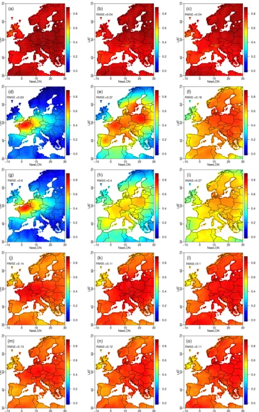
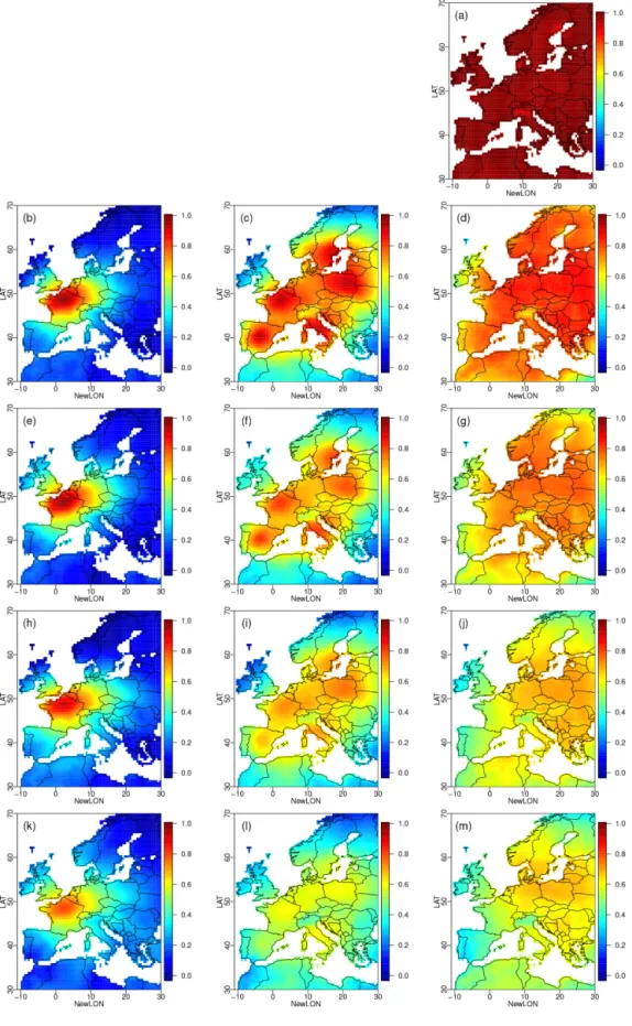
Figure 1. Maps of temperature autocorrelations of the order of 1 d for winter over the 1979–2016 period, for (a) WFDEI, (b) IPSL raw simulations, (c) 1d-BC (CDF-t), (d) R.1.1.0, (e) R.5.1.0, (f) R.100.1.0, (g) R.1.2.0, (h) R.5.2.0, (i) R.100.2.0, (j) R.1.1.1, (k) R.5.1.1, (l) R.100.1.1, (m) R.1.2.1, (n) R.5.2.1 and (o) R.100.2.1. In other words, the second row shows the results for temperature as a conditioning dimension (for different numbers of locations) and without accounting for lags; the third row is the same but for temperature and precipitation together as a conditioning dimension; the fourth and fifth rows are the same as the second and third rows but with lags accounted for. For panels (b–o), the RMSE value, computed over the whole domain between WFDEI autocorrelations and those from the model or corrected data, is indicated.
the reference are located around Paris. The further the points are from Paris, the less the R2D2correction is able to repro-duce the AR1 coefficients observed in the reference. This is explained by two factors. First, the conditioning dimensions in the reference and in BC1D are similar in terms of AR1 co-efficients. Second, in the reference dataset, there is a strong correlation between the conditioning dimension (the temper-ature in Paris) and the tempertemper-ature at sites that are geograph-ically close. Indeed, in R2D2, at each time step we copy the rank association observed in the reference dataset, given the rank of the conditioning variable in the BC1D dataset. Hence, for a site close to Paris, the multivariate correction will al-ter the temperature rank sequence of the reference dataset to make it consistent with the rank sequence of the condi-tioning dimension in the BC1D dataset. In this case, since temperature in Paris in the BC1D dataset possesses temporal properties similar to the references and because of a strong spatial dependence around Paris, the temporal properties of temperature at a site close to Paris will be, after correction, consistent with the temporal properties of the temperature in Paris in the BC1D dataset and, thus, by transitivity, consistent with the temporal properties of the temperature in Paris in the reference dataset. In the following, we will refer to this phe-nomenon as the “transitivity effect”. Note that variables that are independent from (or only weakly correlated to) the con-ditioning dimension in the reference dataset have their ranks altered as well but not necessarily in a meaningful way. In-deed, for independent or weakly correlated variables, the re-arrangement of the rank sequence is equivalent to a random permutation. Hence, to maximize the transitivity effect, it is needed to select conditioning variables (i) that have similar temporal properties in the reference and in the simulations to be corrected and (ii) that, in the reference dataset, show strong dependences with the other variables (i.e., the climate variables at the different sites) that we want to correct. Based on Fig. 1d, it is clear that it is not the case for the temperature in Paris, as already found by Vrac (2018).
However, when increasing the number of sites (R.5.1.0 and R.100.1.0; Fig. 1e and f, respectively) in the condition-ing dimension, an amplification of the transitivity effect is visible: the areas where the AR1 coefficients are well repro-duced have expanded and are located close to the condition-ing sites. Indeed, the mean daily temperature is a relatively smooth signal over this large region and the AR1 coefficients are well represented by the simulations.
Adding precipitation in the conditioning dimension (R.1.2.0, R.5.2.0 and R.100.2.0, respectively, Fig. 1g to i) degrades the AR1 properties compared to having only tem-perature as a conditioning dimension. It may come from the fact that temperature and precipitation may not be strongly dependent and that conditioning on precipitation to find the value of temperatures for points in the neighborhood of con-ditioning sites introduces more noise than signal.
When using lags in the conditioning dimensions, all con-figurations with lags give similar results in terms of RMSE
computed on the AR1 coefficient (RMSE = 0.11) and per-form generally better than the configurations without lags. This could be expected since, in this case, short sequences of ranks in the reference dataset are resampled in the R2D2 corrected dataset. Hence, it mechanically improves the agree-ment between the reference dataset and the R2D2corrected dataset in terms of short-term temporal dependence. This mechanism is the essence of the R2D2philosophy, where we copy, in the multivariate corrected dataset, the rank associa-tion that is given by the condiassocia-tioning dimensions.
Moreover, the configurations using more sites (R.100.1.1 and R.100.2.1) give slightly better results. The spatial vari-ations of the AR1 coefficients are qualitatively better re-spected, with lower values of autocorrelation in Spain, the UK and Libya compared to the rest of the map. Quantita-tively, however, there is a negative bias of about −0.1 on av-erage in terms of AR1 coefficients compared to the reference dataset.
In the end, as the initial temperature simulations have AR1 coefficients similar to those from the references, the IPSL and BC1D simulations show the best temporal properties (best R2D2RMSE = 0.1, BC1D RMSE = 0.04). In terms of temporal correlation, R.1.1.0 (i.e., initial R2D2method) and R.2.1.0 give the worst results with only sensible values of the AR1 coefficient around the Paris area. However, the use of a multivariate conditioning dimension and overall the use of a rank sequence into the conditioning dimensions strongly im-prove the capability of R2D2to account for temporal depen-dence features of the temperature variable. Indeed, the best R2D2results are clearly obtained for configurations account-ing for lags.
4.1.2 Precipitation temporal correlation
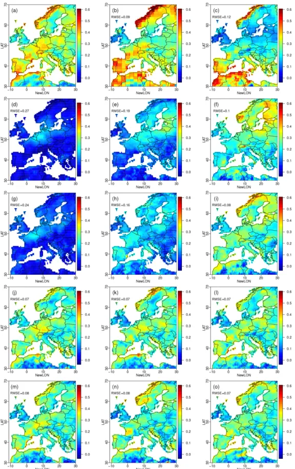
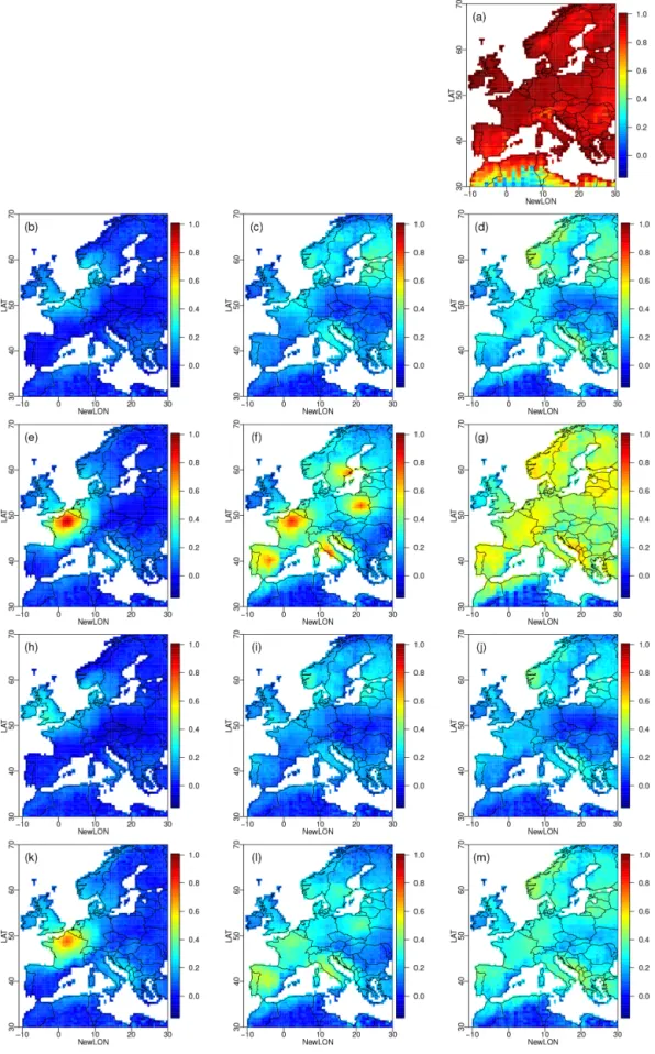
For winter precipitation (Fig. 2), the reference dataset ex-hibits AR1 coefficients with spatial structures smaller than those for temperature. Globally, the model roughly repro-duces the spatial distribution of the AR1 coefficients (IPSL RMSE = 0.09) but clearly lacks spatial resolution. The BC1D results exhibit finer spatial structures, for instance in the northern coastline of Scandinavia. However, the BC1D AR1 coefficients are not as good as those from the IPSL dataset (BC1D RMSE = 0.12). For both IPSL and BC1D, the AR1 coefficients are higher than those for the references in Spain, on the coasts of northern Africa and on the northern coasts of Scandinavia. The agreement between the reference data and the raw simulations in terms of AR1 coefficients is not as good for precipitation as for temperature.
When applying R.1.1.0 – the configuration of R2D2 with the temperature in Paris as a univariate conditioning dimen-sion without lag – the AR1 coefficient is not correctly recon-structed. In most areas, the AR1 coefficient is close to zero, except in Belgium, the Netherlands and northwestern Ger-many where the AR1 coefficient is positive but still nega-tively biased. This probably reveals a rather weak correlation
Figure 2. Same as Fig. 1 but for winter precipitation autocorrelations. Note that here precipitation is never used alone as a conditioning dimension.
between the temperature in Paris and the precipitation in the surrounding area. With R.5.1.0, which adds Madrid, Stock-holm, Rome and Warsaw as conditioning sites, the precipita-tion autocorrelaprecipita-tion is better reconstructed around the added conditioning sites. The effect is notably stronger around War-saw and Stockholm, where the correlation between tempera-ture and precipitation is stronger than in Rome and in Madrid (in general, stronger correlations are observed in northeast-ern Europe in winter; not shown). With R.100.1.0, using 100 conditioning sites, the AR1 coefficient reconstruction is im-proved over all Europe but is still relatively far from the ref-erence.
Adding precipitation in the conditioning dimensions helps to improve the precipitation AR1 coefficient since it is likely that the correlation between precipitation in two close sites is stronger than the correlation between temperature in one site and precipitation in the other site. With 100 condi-tioning sites, geographical features present in the reference dataset start to be visible, for instance, higher AR1 coef-ficients on the coasts of northern Africa and on the north-ern coasts of Scandinavia. Nevertheless, the first-order au-tocorrelations are still biased negatively with respect to the reference dataset. In terms of RMSE, R.1.100.0 performs slightly better than the BC1D dataset (RMSE(BC1D) = 0.12; RMSE(R.1.100.0) = 0.1) and is on the same level as the raw IPSL simulations (RMSE = 0.09), although spatial struc-tures are quite different. The transitivity effect is also limited by the fact that temporal properties of the references and of the BC1D dataset are not so similar. For instance, the AR1 coefficients tend to be lower in the BC1D dataset, both for temperature and precipitation. Such differences necessarily minimize the transitivity effect.
As for the temperature, the configurations of R2D2 using lags in the conditioning dimensions perform better (RMSE =0.07), with performance relatively independent from the number of conditioning sites or the type of climate condition-ing dimensions. In this case, those configurations of R2D2 provide an improvement in terms of RMSE compared to the raw IPSL simulations. Still, the AR1 coefficients are biased negatively compared to the reference dataset: the first-order autocorrelations are globally not as high as in the WFDEI reanalyses. This is also the case for the other seasons, as shown in the Supplement in Figs. S1–S3 for temperature and in Figs. S4–S6 for precipitation.
Hence, depending on the choice of the conditioning di-mensions, R2D2can partially recover temporal properties of the reference dataset, especially when conditioning by lagged information via rank sequences. It is however hard for R2D2 to reconstruct the temporal properties perfectly or even do better than the raw IPSL dataset or the BC1D dataset for tem-perature, a variable whose temporality is already well repre-sented in the model simulations. The improvement brought by R2D2is more pronounced for precipitation temporal prop-erties: including precipitation itself, more conditioning sites or lagged ranks into the conditioning dimension provides
au-tocorrelation values and structures that are more similar to the reference ones than the other datasets are (e.g., raw or BC1D simulations, initial R2D2configuration R.1.1.0).
Generally, as seen in this section, although the proposed extensions clearly improve the initial R2D2method in terms of temporal correlations, the latter can present some underes-timation of the temporal properties of the reference dataset, both for temperature and precipitation. This could be linked to an inhomogeneous sampling of the rank associations that are taken from the reference dataset. This is thus investigated in the next section (Sect. 4.2).
4.2 Reference time sampling and model chronology agreement
When the conditioning dimension is univariate and continu-ous, with unique ranks (i.e., no repetitions of values) and be-longs to the variables to be corrected, it is the only variable (from the BC1D dataset) that the R2D2resampling scheme does not modify. Therefore, in this case, if the number of days is the same in the reference and model dataset, each time step is sampled exactly once and they are uniformly se-lected. Hence, in this specific case, R2D2reproduces exactly the inter-site and inter-variable empirical copula of the refer-ence but not the temporal dependrefer-ences of the data.
However, when the conditioning has a dimension equal to or greater than 2, there is no guarantee that the exact same rank associations exist in the reference dataset. Indeed, the higher the dimension of the conditioning, the less probable it is to find the exact rank association in the reference and in the BC1D dataset. This can come from either (i) a sampling issue: the higher the dimension, the more points are needed to uniformly sample the space or (ii) from biases in the de-pendence structure (biases in the rank associations) of the conditioning dimension in the dataset to be corrected. In this case, R2D2uses the rank associations of the reference dataset that is the closest in terms of Euclidean distance. Hence, the rank association of the conditioning dimension in the result-ing R2D2 dataset can be different from that of the BC1D dataset. One consequence is that some time steps (i.e., days in our case) can be resampled several times, while others might not be sampled at all. This can obviously have consequences on the properties (marginal, inter-site, spatial, temporal) of the multivariate corrections.
Therefore, we now analyze the distributions of the time steps that have been selected, since it is an indicator of po-tential biases introduced by the analogue-resampling scheme in R2D2.
To reproduce exactly the empirical copula of the reference dataset, each time has to be selected only once. The more un-even the distribution of selected time steps, the more likely it is that the correction has modified the frequency of some sit-uations with respect to the reference dataset. However, there is not a direct relationship between the unevenness of the dis-tributions and the biases introduced in the correction. For
in-stance, if some rank associations do not appear in the cor-rection, they could have been substituted by a very similar association. In this case, the bias introduced would be very small.
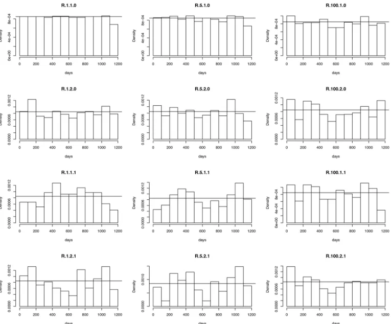
The distributions of time steps selected in the reference dataset in January by the different configurations of R2D2are shown in Fig. 3 (the distributions for April, July and October are provided in Figs. S7–S9). As expected, R.1.1.0 presents a uniform histogram, since it uses a univariate conditioning that permits the sampling of the whole reference time steps. However, this is not the case for the other configurations of R2D2, which all have dimensions of the conditioning equal to or greater than 2 (see Table 1). For the configurations of R2D2with only temperature as the conditioning dimension and without time lags (R.5.1.0, R.100.1.0), the sampling is quite uniform. This suggests that the spatial properties of the temperature are quite similar between the reference dataset and the BC1D dataset. When adding the precipitation as the conditioning dimension without time lags (R.2.1.0, R.2.5.0, R.2.100.0), the histograms are slightly less uniform. This in-dicates that there can be discrepancies between the references and the BC1D dataset for the spatial dependence of itation or the dependence between temperature and precip-itation. Finally, when adding time lags in the conditioning dimensions, both for temperature and precipitation (R.1.1.1, R.1.2.1, R.1.100.1, R.5.1.1, R.5.2.1, R.5.100.1), the distribu-tions of selected times also appear to be less uniform. This is especially true for R.5.2.1, where we observe a trough in the distribution between days 600 and 700. It indicates that the modeled rank sequences in this period rarely appear in the BC1D dataset.
Those elements can help us to interpret the performance of the different configurations of R2D2 with respect to the reconstruction of temporal, spatial and marginal properties of the temperature and precipitation fields.
Moreover, in order to see how much the different R2D2 configurations change the temporal structures of the origi-nal raw simulations, for all sites and climate variables, we have computed the correlation between the ranks of the ini-tial raw simulations and the ranks of the multivariate cor-rected time series. The closer the correlation is to 1, the less R2D2has modified the temporal structures of the raw simu-lations. The correlation coefficients for the different sites in winter are shown in Figs. 4 for temperature and 5 for pre-cipitation. The other seasons are shown in Figs. S10–S15 in the Supplement. By construction, the CDF-t BC1D mostly conserves the ranks of the raw simulations.
For temperature (Fig. 4), we see that the time series of ranks have been modified substantially by R.1.1.0 (Fig. 4b). When the number of geographical sites increases (R.5.1.0 and R.100.1.0; Fig. 4c and d), we observe the transitive effect and the rank time series are more correlated to those from raw simulations. It is made possible because the variations of temperature are spatially smooth and because the references
and BC1D data seem to have similar temperature temporal properties.
The transitivity effect is also seen when precipitation is added as a conditioning dimension (R.1.2.0, R.5.2.0, R.100.2.0; Fig. 4e–g) or when time lags are added (R.1.1.1, R.5.1.1, R.100.1.1, R.1.2.1, R.5.2.1, R.100.2.1; Fig. 4h–m). However, fewer changes are made in the rank time series when the number of conditioning sites increases. However, for those versions of R2D2with a high number of condition-ing sites, the resultcondition-ing rank time series are slightly more mod-ified (i.e., rank correlation further away from 1) than with just the temperature as the conditioning dimension. It may come from the fact that the higher the dimension of the condition-ing, the more likely the rank sequence of the conditioning dimension has to be modified.
For precipitation (Fig. 5), similar observations can be made. However, the changes in the rank time series are larger than for temperature. It can be partially explained by the fact that the transitivity effect is weaker for precipitation. Indeed, precipitation events occur at local scale and with a spatial correlation radius smaller than for temperature.
Globally, due to the transitivity effect, sites strongly corre-lated with the conditioning dimension in the reference dataset have their rank sequences mostly conserved after the cor-rection if the conditioning dimension has similar temporal properties in the reference and the model. As a consequence, adding more sites in the conditioning dimension generally leads to more regions that mostly preserve the rank sequences of the model. However, to some extent, this effect can be counteracted by the fact that, as the dimension of the condi-tioning grows (e.g., adding rank lags in the condicondi-tioning), it becomes harder to find the exact rank associations in the ref-erence data. It leads to alterations in the rank sequences for the conditioning dimension and for the sites that are corre-lated with it, and finally to a potential decrease of the rank correlation between the raw simulations and their correc-tions.
4.3 Marginal, spatial and inter-variable evaluations As seen previously, some of the proposed R2D2extensions allow us to adjust temporal dependence structure. How-ever, as the initial R2D2 method was designed to bias cor-rect multi-site and inter-variable dependences in addition to marginal distribution, one can wonder how the temporal structure improvements – as well as the time-sampling fea-tures – made by the R2D2extensions impact the corrections performed on the other dependences, i.e., whether or not they degrade the marginal, spatial and inter-variable properties. This is the purpose of Sect. 4.3.1 (marginal), 4.3.2 (inter-variable) and 4.3.3 (spatial).
Figure 3. Distributions of time steps selected in the reference dataset in January by the different R2D2 configurations. The equivalent histograms for April, July and October are provided in the Supplement in Figs. S7–S9.
4.3.1 Marginal properties
We first check whether the R2D2correction schemes are able to reconstruct the marginal properties of the reference dataset through two statistics: the mean and the standard deviation.
For each season and each grid point, biases in mean temperatures have been computed and are shown in Fig. 6 as boxplots. The associated maps are given in Figs. S16–S19. For all seasons, there are clear differ-ences between the reference and the IPSL simulations (1.58 < RMSE < 1.84◦C). The best performance is achieved by BC1D (0.08 < RMSE < 0.2◦C), although some light pos-itive or negative biases may appear on some regions, depend-ing on the season (see Figs. S16–S19). This strong improve-ment of CDF-t over the raw simulations was expected as the
univariate BC focuses on reconstructing the marginal distri-bution of the reference.
R.1.1.0 provides similar performance. Since the condition-ing dimension is univariate, R2D2only performs a permuta-tion of the ranks in time. It then only corresponds to a time reordering of the BC1D correction and does not affect the marginal distributions.
On average, going from one conditioning site to five, with R.5.1.0, increases the biases in mean (0.13 < RMSE < 0.24◦C). However, using 100 sites (R.100.1.0) is equivalent to five in terms of mean (0.13 < RMSE < 0.22◦C). Yet, the degradation is more visible when adding precipitation into the conditioning dimensions and when increasing the number of conditioning sites to 100. For R.100.2.0, the RMSE is between 0.19 and 0.54◦C depending on the season, and biases can locally
Figure 4. Maps of Spearman (rank) correlations calculated for each grid point in winter over 1979–2016 between the initial climate model temperature simulations and their corrections by (a) 1d-BC, (b) R.1.1.0, (c) R.5.1.0, (d) R.100.1.0, (e) R.1.2.0, (f) R.5.2.0, (g) R.100.2.0, (h) R.1.1.1, (i) R.5.1.1, (j) R.100.1.1, (k) R.1.2.1, (l) R.5.2.1 and (m) R.100.2.1. The results for the other seasons are provided in the Supplement.
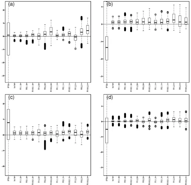
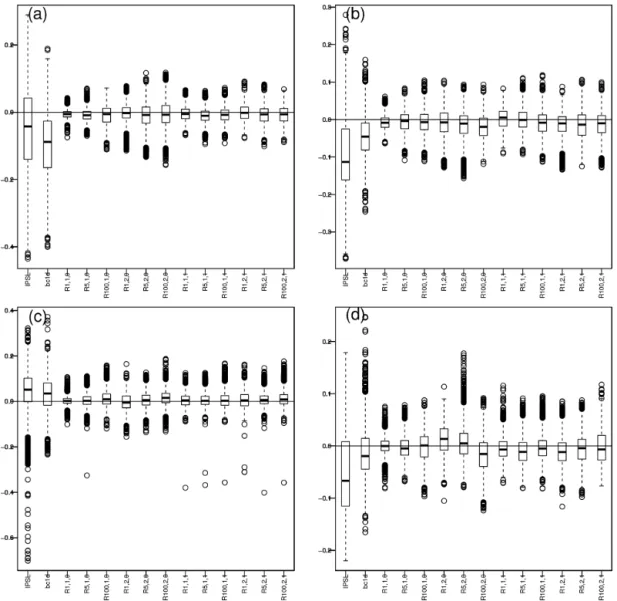
Figure 6. Boxplots of differences in mean temperature per grid point with respect to WFDEI, i.e., mean(model or BC) minus mean(WFDEI): (a) winter, (b) spring, (c) summer and (d) fall. The associated maps are given in Figs. S16–S19.
exceed 0.5 or even 1◦C in winter over eastern Europe, for instance (Fig. S16i). It can be linked to the fact that for R.100.2.0, the distribution of time steps selected is less uniform (Fig. 3), hence, modifying the marginal mean values provided by CDF-t.
Similar observations can be made when looking at R2D2 corrections accounting for lags in the conditioning dimen-sion. Configurations including precipitation have less uni-form distributions of selected time steps and have thus higher biases.
Somehow similar patterns of biases also occur when look-ing at the standard deviation of the temperatures (Fig. S20).
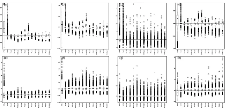
For precipitation, univariate biases are investigated in sep-arating occurrences of rainfall and conditional intensities given rainfall occurrences. Hence, Fig. 7 displays, for the four seasons, boxplots of the relative differences of the prob-abilities of rainfall occurrence with respect to that of the
ref-erence data (Fig. 7a–d), as well as the boxplots of relative differences of the mean conditional intensities given rain-fall occurrences, with regard to that of the reference data (Fig. 7e–h). The associated maps are given in the Supple-ment (Figs. S21–S24 for occurrence probabilities and S25– 28 for mean conditional intensities). Rainfall occurrences are defined as precipitation values > 0.1 mm d−1 to get rid of the drizzle effect present in many climate model simula-tions (e.g., Dai, 2006; Kjellström et al., 2010; Teutschbein and Seibert, 2012). Generally speaking, the effects of R2D2 on the occurrence and conditional mean precipitation biases are similar to those observed on the mean temperature: (i) the R.1.1.0 configuration provides similar performance to BC1D, (ii) with or without time lags and with or without adding precipitation in the conditioning, increasing the num-ber of conditioning sites may lead to relatively higher biases, both for occurrence probability and intensity. However,
in-cluding precipitation itself in the conditioning does not am-plify the precipitation biases and can even reduce them de-pending on the season.
Biases in standard deviations for conditional precipitation values are also given for information (Fig. S29) and coincide with results for means.
Generally, for both temperature and precipitation marginal properties, the biases tend to be stronger for R2D2 configu-rations that exhibit non-uniform sampling of the time steps selected.
4.3.2 Inter-variable correlations
We now evaluate the capability of the different R2D2 config-urations to adjust inter-variable dependences. We first com-pute the Pearson correlation between temperature and pre-cipitation for each grid point in the corrected dataset. We then compare these correlation values with those from the references. The results are summarized as boxplots of differ-ences in correlation (Fig. 8). The associated maps are given for each season in Figs. S30–S33 in the Supplement. Note that the Spearman rank correlation analysis provides simi-lar conclusions, although they are perturbed by the rare rain-fall occurrences, especially over northern Africa (not shown), which complicates the analysis of the boxplots. Indeed, daily precipitation data contain many zeros and therefore many tied first ranks. In a case with, for example, 100 values whose 80 % are zeros, 80 ranks are ties and equal to 1, while the first rank not equal to 1 is the 81st, creating a “jump” in the rank distribution. A relatively small error in the rainfall occur-rence frequency can then lead to a high bias in the Spearman (rank) correlation, while the Pearson correlation is less sen-sitive since it is based on “real” values and not ranks. Hence, the Pearson correlation has been preferred.
In the IPSL model and in the BC1D correction, the corre-lation between temperature and precipitation is weaker than in the reference dataset. We expect R.1.1.0 to have the best performance with regards to inter-variable rank correlation. Indeed, it has a univariate conditioning dimension, implying that the empirical copula between temperature and precipi-tation of the reference data observed during the calibration periods is reproduced almost exactly. In practice, in Fig. 8, the boxplots for R.1.1.0 are not exactly 0. It indicates that in the references, the empirical copula between tempera-ture and precipitation is not exactly the same during the two time periods used alternatively for calibration and validation. However, R.1.1.0 (i.e., the initial R2D2method) is the main benchmark of the inter-variable evaluation. Indeed, it was de-signed to adjust the temperature–precipitation dependence of the raw simulations, which is the case since it strongly im-proves IPSL and BC1D dataset properties. Then, the simi-lar behaviors of the different R2D2 configurations indicate that their T2 vs. PR correlations are also improved and in a similar way. In other words, for all R2D2extensions, includ-ing those improvinclud-ing the temporal dependence structures (see
Sect. 4.1), the inter-variable correlation is not degraded with respect R.1.1.0 and therefore satisfyingly corrected.
4.3.3 Spatial correlations
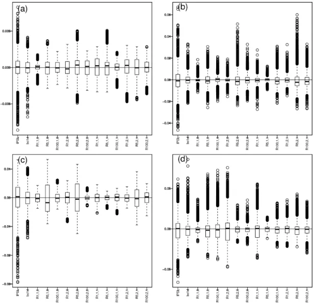
Finally, we evaluate the spatial correlation by computing the loading values of the first empirical orthogonal function (EOF) obtained from a principal component analysis (PCA) applied on temperature and precipitation separately. For each dataset, we compare the associated loading values with those obtained for the references. The results for winter and sum-mer are summarized in Fig. 9 as boxplots drawn from differ-ences of loading values between the R2D2 corrections and the WFDEI references. The associated maps are given in Figs. S34–S37 in the Supplement.
For both temperature and precipitation, and for all seasons, the raw IPSL simulations have loading values well centered around those of WFDEI since the median of the differences is close to 0.
Simply by correcting the marginal distribution, BC1D im-proves the agreement with the reference dataset. Indeed, EOFs are computed from the variance–covariance matrix, which is sensitive to the change in the marginal distributions. In the R2D2configurations, as already explained, the ranks of the non-conditioning variables are shuffled to match those in the reference dataset during the calibration period. If the inter-site copula is similar during the calibration and vali-dation periods, the R2D2configurations should improve the spatial correlations compared to BC1D. This is the case for R.1.1.0, as well as for other configurations, where the me-dian of the difference is close to 0 and where an interquartile range of the differences is narrower than that for BC1D. In-terestingly, the configurations with the largest interquartile range are those for which the sampling of the time steps is less uniform (Fig. 3), illustrating again the potential impacts of an uneven sampling. However, many R2D2configurations are able to reconstruct spatial properties correctly, at least as well as the initial R2D2method (i.e., with a univariate condi-tioning dimension) that was explicitly designed for it. This is even more visible when looking at the maps of loading values (Figs. S34–S37). Hence, the introduction of additional condi-tioning information into R2D2– needed to improve temporal properties as seen in Sect. 4.1 – does not degrade much the capability of R2D2to adjust the spatial dependence structures of the climate simulations.
Spatial correlograms are not shown but clearly indicate similar results.
5 Conclusions and discussion 5.1 Conclusions
To fill some needs of the climate change impact commu-nity, an MBC method has been proposed in this study. In addition to marginal properties, this MBC is designed to
ad-Figure 7. (a–d) Boxplots of relative differences of the probabilities of rainfall occurrence with respect to that of the reference data; (e–h) boxplots of relative differences of the mean conditional intensities given rainfall occurrences, with regard to that of the reference data. The results are given for winter (a, e), spring (b, f), summer (c, g) and fall (d, h). To get rid of the drizzle effect, the threshold for precipitation occurrence is set to 0.1 mm d−1. Associated maps are given in Figs. S21–S24 for occurrence probabilities and Figs. S25–S28 for mean conditional precipitation.
just both the inter-site and inter-variable dependence struc-tures of climate simulations and at the same time to improve the temporal properties of the corrections. Our approach is based on the previously existing R2D2method (Vrac, 2018) that relied on a univariate “conditioning dimension” to sam-ple ranks from a reference dataset and therefore reconstruct the copula-based spatial and inter-variable dependences. The suggested R2D2extensions allow resampling ranks given a multivariate conditioning dimension, which could be ranks of multiple physical variables at a time step t , ranks from a single physical variable but over a sequence of N time steps (t −(N −1), . . ., t ) or ranks of multiple physical variables over a sequence of N time steps.
Several configurations (i.e., different conditioning dimen-sions including different sites and climate variables, with or without lagged information) have been applied to correct daily precipitation and temperature simulations over Europe from a single climate model run, the IPSL-CM5 Earth sys-tem model (Marti et al., 2010; Dufresne et al., 2013), with respect to the WFDEI data (Weedon et al., 2014) as refer-ences. As the initial R2D2approach by Vrac (2018) was able to properly adjust spatial and inter-variable structure but not the temporal properties of the simulations, the underlying question of the present study was to understand (i) if the pro-posed multidimensional conditioning in R2D2improves the temporal aspects of the corrections and (ii) the impact of this conditional resampling on the adjustment quality of the other (i.e., marginal, spatial, inter-variable) properties. Hence, the
various R2D2 configurations have been evaluated and com-pared to the raw simulations as well as to corrections from the univariate BC method CDF-t (e.g., Vrac et al., 2012), first in terms of autocorrelation to characterize the main temporal aspects and then in terms of marginal properties, spatial de-pendences and temperature vs. precipitation correlations.
For temporal properties, although the R2D2 variants strongly improve the initial R2D2approach, they do not reach the rather good level obtained for temperature with the tested 1d-BC (due to the correct auto-correlations from the raw temperature simulations), while the results are more debat-able for precipitation. In general, the main conclusions were that including more information (sites and/or lagged ranks) in the conditioning dimension generally improves the recon-struction of the autocorrelation coefficients, both for temper-ature and precipitation. However, when the dimension of the conditioning (i.e., the number of variables, sites and lags to condition the resampling) increases, the distribution of the sampled time steps can be quite different from the uniform one. This has then consequences mostly on the marginals (i.e., univariate properties), where the mean and standard de-viation can have stronger biases for non-uniform sampling. For the other evaluations (spatial and inter-variable proper-ties), although variations in the results are visible depending on the conditioning dimension used, the main conclusion is that the proposed R2D2configurations are relatively stable. Thus, in general, the introduction of additional conditioning information into R2D2allows improving temporal properties
Figure 8. Boxplots of differences in temperature vs. precipitation Pearson correlations between WFDEI and the different datasets (IPSL, 1d-BC IPSL and the R2D2configurations) over 1979–2016 in (a) winter, (b) spring, (c) summer and (d) fall. The associated maps are given for each season in the Supplement.
with a good preservation of the capability of the initial R2D2 to adjust both the spatial and inter-variable dependences of the raw simulations. Hence, in practice, we recommend a “compromise setting” in the choice of the conditioning di-mension, with not too few and not too many sites. Such a choice would prevent both from missing transitivity effects and from having an uneven time step distribution.
5.2 Discussion and perspectives
The method suggested in this study is of course upgradable along different axes.
First, as our goal was not to test the various R2D2 con-figurations on several climate models but rather to establish a proof of concept of the R2D2 extension on an illustrative simulation run, only one climate model has been used for ap-plication and evaluation in the present study. Although we
hypothesize that the main general findings obtained on this single model application will still be valid for other models and simulations, this will need to be confirmed to generalize and refine our results to more model simulations.
Moreover, the fundamental assumption of R2D2is that the spatial and inter-variable copulas (i.e., rank association) is stationary in time, even for future climate projections. This assumption – considering that rank associations act as prox-ies of physics (Vrac, 2018) and that physics does not change in time – is nevertheless debatable since it needs to be ver-ified in further works. However, it highlights the fact that the conditioning dimension has to be carefully chosen to be relevant, both to drive (i.e., condition) the correction of the properties of interest and to translate the potential changes that may happen in future climate and that would impact the corrections. Hence, the potential non-stationarity of the de-pendences between climate variables (i.e., rank association)
Figure 9. Boxplots of differences in loading values for the first EOF (EOF1) between model or corrected data and WFDEI (i.e., EOF1(model or BC) minus EOF1(WFDEI)). Panels (a) and (c) are for temperature, (b) and (d) for precipitation, for winter (a, b) and summer (c, d). The associated maps are given in the Supplement.
may be worth exploring further. This could be done via sev-eral questions; e.g., how stable is the rank association with time? How long does the considered period have to be in or-der to faithfully estimate the association? How can climate change alter it? Those questions, however, are not specific to our suggested method. They concern many methods and studies relying on dependences of climate variables in cli-mate change contexts. Such fundamental questions deserve to be investigated on their own and are thus left for future works.
More generally, the choice of the conditioning dimension is a key element of the R2D2method. Indeed, as seen in this study, what is corrected or not by R2D2 is partially driven by the chosen conditioning information. Thus, testing alter-native conditioning dimensions could also be of interest for future work, to bring additional physical/geographical infor-mation, valuable to generate proper multivariate corrections.
This alternative conditioning – e.g., including NAO or other indices, characterization of the circulation or other covariates – nevertheless has to be determined according to the specific region of interest, the climate variables to be corrected, etc. This adaptation of the conditioning to the application is a requirement to inject the relevant and suited physical infor-mation into R2D2.
Of course, if a “good” conditioning must optimize the R2D2correction of some statistical properties, it mainly has to optimize the properties that are the most useful for the users of the corrections. In other words, the choice of the R2D2 configuration has to be tailored for the end users of the simulations. It is thus very important for the end users to know which properties are essential to be corrected in order to design the R2D2configuration that is most appropriate for their specific application. Indeed, if many statistical features of the simulations are to be corrected, it is not clear that a
single configuration will be able to correct all properties. For some regions and sets of climate variables, this can happen, but in other cases it might be needed to prioritize the most essential ones and then choose the associated R2D2 configu-ration.
Finally, trying to correct multiple statistical properties at the same time remains a difficult challenge, as adjusting one often modifies another one. Additionally, one can wonder what is kept from the raw climate simulations if a correc-tion is performed to adjust many statistical aspects. Hence, when applying a multivariate bias correction method with a configuration allowing us to modify (explicitly or implicitly) several properties, a compromise has to always be searched in order to balance, on the one hand, the level of correction needed to make the simulations useful for the application of interest and, on the other hand, the climate model signal pre-served by the applied correction method. This is the only way to make the (M)BC useful in practice and physically reliable.
Code and data availability. The R2D2 code (Vrac and Thao, 2020), specifically developed for this study and used to adjust the dependence structure of the 1d-BC data, is available as an R package (“R2D2”) under the CeCILL license and is available for download at https://doi.org/10.5281/zenodo.4021981 (Vrac and Thao, 2020). This package includes the source code, example data and a user manual. The IPSL-CM5A-MR model data simulations as part of the CMIP5 climate model simulations can be down-loaded through the Earth System Grid Federation portals. Instruc-tions to access the data are available here: https://pcmdi.llnl.gov/ mips/cmip5/data-access-getting-started.html, last access: 10 Febru-ary 2019, (PCMDI, 1989). The WFDEI data used as reference in this study can be accessed following the instructions described in Weedon et al. (2018) or at https://doi.org/10.5065/486N-8109.
Supplement. The supplement related to this article is available on-line at: https://doi.org/10.5194/gmd-13-5367-2020-supplement.
Author contributions. MV had the initial idea for the method, de-veloped the associated code and made the figures. ST wrapped the R package. MV and ST performed the analyses and wrote the article.
Competing interests. The authors declare that they have no conflict of interest.
Acknowledgements. We acknowledge the World Climate Research Programme’s Working Group on Coupled Modelling, which is re-sponsible for CMIP, and we thank the IPSL climate modeling groups for producing and making available their model output. For CMIP, the US Department of Energy’s Program for Climate Model Diagnosis and Intercomparison provides coordinating sup-port and led development of software infrastructure in partnership with the Global Organization for Earth System Science Portals.
Fi-nally, Mathieu Vrac would like to thank Pascal Yiou (LSCE) for fruitful discussions about analogues.
Financial support. This work has been supported by the EU-PHEME and CoCliServ projects, both part of ERA4CS, an ERA-NET initiated by JPI Climate and co-funded by the European Union (grant no. 690462).
Review statement. This paper was edited by Simone Marras and re-viewed by Sylvie Parey and Verena Bessenbacher.
References
Bellard, C., Bertelsmeier, C., Leadley, P., Thuiller, W., and Cour-champ, F.: Impacts of climate change on the future of biodi-versity, Ecol. Lett., 15, 365–377, https://doi.org/10.1111/j.1461-0248.2011.01736.x, 2012.
Ben-Ari, T., Boé, J., Ciais, P., Lecerf, R., Van der Velde, M., and Makowski, D.: Causes and implications of the unforeseen 2016 extreme yield loss in the breadbasket of France, Nat. Commun., 9, 1627, https://doi.org/10.1038/s41467-018-04087-x , 2018. Bevacqua, E., Maraun, D., Vousdoukas, M., Voukouvalas, E., Vrac,
M., Mentaschi, L., and Widmann, M.: Higher probability of com-pound flooding from precipitation and storm surge in Europe under anthropogenic climate change, Sci. Adv., 5, eaaw5531, https://doi.org/10.1126/sciadv.aaw5531, 2019.
Boé, J., Terray, L., Habets, F., and Martin, E.: Statistical and dynamical downscaling of the Seine basin climate for hy-dro-meteorological studies, Int. J. Climatol., 27, 1643–1655, https://doi.org/10.1002/joc.1602, 2007.
Brown, C. J., Schoeman, D. S., Sydeman, W. J., Brander, K., Buckley, L. B., Burrows, M., Duarte, C. M., Moore, P. J., Pan-dolfi, J. M., Poloczanska, E., Venables, W., and Richardson, A. J.: Quantitative approaches in climate change ecology, Glob. Change Biol., 17, 3697–3713, https://doi.org/10.1111/j.1365-2486.2011.02531.x, 2011.
Cannon, A.: Multivariate quantile mapping bias correction: An N-dimensional probability density function transform for climate model simulations of multiple variables, Clim. Dyn., 50, 31–49, https://doi.org/10.1007/s00382-017-3580-6, 2017.
Cannon, A. J., Sobie, S. R., and Murdock, T. Q.: Bias Correction of GCM Precipitation by Quantile Mapping: How Well Do Methods Preserve Changes in Quantiles and Extremes?, J. Climate, 28, 6938–6959, https://doi.org/10.1175/JCLI-D-14-00754.1, 2015. Christensen, J., Boberg, F., Christensen, O., and Lucas-Picher, P.:
On the need for bias correction of regional climate change pro-jections of temperature and precipitation, Geophys. Res. Lett., 35, L20709, https://doi.org/10.1029/2008GL035694, 2008. Christensen, N. S., Wood, A. W., Voisin, N.,
Letten-maier, D. P., and Palmer, R. N.: The Effects of Climate Change on the Hydrology and Water Resources of the Colorado River Basin, Climatic Change, 62, 337–363, https://doi.org/10.1023/B:CLIM.0000013684.13621.1f, 2004. Ciais, P., Reichstein, M., Viovy, N., Granier, A., Ogée, J.,
Al-lard, V., Aubinet, M., Buchmann, N., Bernhofer, C., Carrara, A., Chevallier, F., De Noblet, N., Friend, A. D., Friedlingstein,