HAL Id: halshs-01651042
https://halshs.archives-ouvertes.fr/halshs-01651042
Submitted on 28 Nov 2017
HAL is a multi-disciplinary open access
archive for the deposit and dissemination of
sci-entific research documents, whether they are
pub-lished or not. The documents may come from
teaching and research institutions in France or
abroad, or from public or private research centers.
L’archive ouverte pluridisciplinaire HAL, est
destinée au dépôt et à la diffusion de documents
scientifiques de niveau recherche, publiés ou non,
émanant des établissements d’enseignement et de
recherche français ou étrangers, des laboratoires
publics ou privés.
Under Risk, Over Time, Regarding Other People:
Language and Rationality Within Three Dimensions
Dorian Jullien
To cite this version:
Dorian Jullien. Under Risk, Over Time, Regarding Other People: Language and Rationality Within
Three Dimensions. Research in the History of Economic Thought and Methodology, Elsevier, 2018,
36 (C). �halshs-01651042�
Under Risk, Over Time, Regarding Other People:
Language and Rationality Within Three Dimensions
Dorian Jullien
∗September 1, 2017
Abstract
This paper conducts a systematic comparison of behavioral economics’s challenges to the standard accounts of economic behaviors within three dimensions: under risk, over time and regarding other people. A new perspective on two underlying methodological issues, i.e., interdisciplinarity and the positive/normative distinction, is proposed by following the entanglement thesis of Hilary Putnam, Vivian Walsh and Amartya Sen. This thesis holds that facts, values and conventions have interdependent meanings in science which can be understood by scrutinizing formal and ordinary language uses. The goal is to provide a broad and self-contained picture of how behavioral economics is changing the mainstream of economics.
Keywords: behavioral economics, economic rationality, expected utility, prospect the-ory, exponential discounting, hyperbolic discounting, self-interest, other-regarding behav-iors, economic methodology, history of economics, philosophy of economics, economics and language
JEL: A12, B21, B41, D01, D03, D81, D90, D64
Introduction
The intended contribution of this paper is to provide a broad picture of how behavioral eco-nomics is changing the mainstream of our discipline. Behavioral ecoeco-nomics stems from the ∗Université Côte d’Azur, CNRS, GREDEG, France. [email protected]. I thank Samuel Ferey,
Peter Wakker, Nicolas Vallois, Wade Hands, Kevin Hoover and two anonymous referees for their comments on earlier drafts of this paper, along with the participants to the 2015 Thurstone Workshop in Paris. This paper is a revision of a part of my Ph.D. dissertation (chap.2, sect. 1) and a few developments on risk preferences in section 3 are also used in a previsouly published paper (in Œconomia, 6-2, 2016, 265-291).
influence, in the late 1970s, of psychologists Daniel Kahneman and Amos Tversky on economist Richard Thaler. Since then, behavioral economists borrow psychologists’ experimental meth-ods and theoretical concepts to study various empirical departures of individual behaviors from the predictions of standard models. Most contributions in behavioral economics focus on three dimensions of economic rationality, which are often expressed differently depending on one’s audience. Addressing economists, Stefano DellaVigna uses the language of preferences: “[t]he first class of deviations from the standard model [...] is nonstandard preferences [...] on three dimensions: time preferences, risk preferences, and social preferences” (2009, p.316). Address-ing scholars from other disciplines, Thaler and his co-authors stress “Three Bounds of Human Nature” (Mullainathan and Thaler 2001, p.1095), namely that “people exhibit bounded ratio-nality, bounded self-interest, and bounded willpower” (Jolls, Sunstein and Thaler 1998, p.1471). In both cases, these authors are saying that behavioral economics mainly challenges standard models of individual behaviors under risk, over time and regarding other people.1
Alternative models from behavioral economics can be seen as modifications – conceptually inspired from psychology – to standard models. The most popular ones are reprinted in Advances
in Behavioral Economics (Camerer, Loewenstein and Rabin 2004). There again, a large part of
the “basic topic” is organized in terms of “preferences over risky and uncertain outcomes”, “in-tertemporal choice” and “fairness and social preferences” (ibid, table of content). This threefold distinction is not new. It organizes numerous classics of standard economics, albeit in a less salient fashion (see e.g., Deaton and Muellbauer 1980; Mas-Colell et al. 1995). It is, however, increasingly used in a systematic way by prominent standard economists writing on behavioral economics (e.g., Fudenberg 2006; Pesendorfer 2006; Levine 2012). Despite the large number of contributions from historians, philosophers and methodologists on issues related to behavioral economics, there is no reflexive perspective on the centrality of this threefold distinction. This paper conducts a historically-motivated and methodologically-oriented comparison of the three ways behavioral economics shaped itself within each dimension.
The historical motivation is to give an account of the empirical and theoretical state of affairs 1In terms of Sent’s (2004) distinction, this paper is only about the “new” behavioral economics of Kahneman,
Tversky, Thaler and others but not the “old” one initiated by Simon. Connections and contrasts between these two traditions are discussed elsewhere (see, e.g., Sent 2004; Klaes and Sent 2005, esp. p.47; Egidi 2012; Kao and Velupillai 2015; Geiger 2016). On the systematic deviations that are not about the three dimensions but contradict directly the bedrock of consumer choice theory under certainty (in the sense of Mas Collel et al. 1995, chaps. 1-3), see Thaler (1980; 2015, parts. I-II).
around behavioral economics before the second half of the 2000s. Before this period, behav-ioral and standard economists focused on either one of the three dimensions taken separately from the other two. After this period, the focus is also on what happens when at least two dimensions are interacting. In other words, there is a shift of focus from contributions within the three dimensions to contributions across the three dimensions. This shift is arguably of historical significance because it produces opportunities for a reconciliation between standard and behavioral economics. Contributions across the three dimensions are however too numer-ous and disorganized to be discussed here. The historical scope of this paper is conceptual, not chronological, i.e., it also uses post mid-2000s contributions within the three dimensions to better understand the conditions of possibility of the contemporary shift – not the shift itself.2 The methodological orientation is to provide a new perspective on two interrelated issues underlying the rise of behavioral economics. On the one hand, there is the positive/normative issue, which is about the meaning of economic rationality in the interplay between (positive) observations of individual behavior and (normative) judgments of these observations as rational or not. On the other hand, there is the issue of interdisciplinarity, which is about the way behavioral economists borrow from psychologists to modify standard economics’s models. The new perspective on these two issues consists in scrutinizing the role of language uses by both economists and economic agents, especially about the three dimensions of risk, time and other people and their associated psychological terms. The first section of the paper presents this methodological perspective in some details, which is then used throughout the paper. The second one compares the main empirical challenges that have motivated behavioral economists’ work on the three dimensions. The third one discusses the common denominator to these challenges, namely that they all violate instances of the consequentialism inherent to standard models. The last one compares behavioral economics’s main theoretical alternatives in the three dimensions. Finally, a conclusion briefly summarizes the arguments and suggests further researches of historical, methodological and philosophical interests.
There are three limits to the broadness of the picture presented here due to space constraints. Firstly, it focuses much more on the qualitative challenges from behavioral economics than on 2Representatives of the shift to contributions across dimensions include Abdellaoui et al. (2013), Andersen et
al. (2008), Andreoni and Sprenger (2012), Baucells and Heukamp (2012), Bolton and Ockenfels (2010), Epper and Fehr-Duda (2015), Halevy (2008), Kovarik (2009), Saito (2013), Trautmann and Vieider (2012).
the quantitative ones. Qualitative challenges are inconsistent behaviors that violate some axioms underlying the standard models, making it impossible to represent those behaviors by one utility function. Quantitative challenges are behaviors that can be captured by one such function but at the price of implying absurd numerical values and degrees of curvature (interpreted as measures of risk, time and/or social preferences in different situations, see Broome 1991). Secondly, it focuses on decision theoretic issues at the expense of game theoretic ones. Hence the dimension of other people is investigated in its simplest forms. Thirdly, it focuses on probabilistic risk at the expense of non-probabilistic uncertainty.3
1
Methodological Perspective
Both behavioral economists and commentators in history, methodology and philosophy of eco-nomics remark that the rise of behavioral ecoeco-nomics comes with a use of the positive/normative distinction that is different from the traditional one (see, e.g., Thaler 1980; Heukelom 2011; 2012; 2014; Hands 2015). The traditional use of the distinction is to separate a positive economics describing, explaining or predicting economic states of affairs from a normative economics evalu-ating, recommending or prescribing economic states of affairs (Mongin 2006a). Here ‘normative’ takes an ethical meaning: economists make or study ethical value judgments, i.e., about what is good, fair, just and so on. Furthermore, the main objects of discussion are collective forms of be-havior or rationality and the evaluation of market efficiency. The different use of the distinction associated with the rise of behavioral economics is to separate a positive from a normative inter-pretation of models of individual behavior. On a positive interinter-pretation, such models describe, explain or predict the behavior of an individual. On a normative interpretation, they evaluate, recommend or prescribe rational behavior. Hence, ‘normative’ here does not (at least directly) takes an ethical meaning: economists make or study value judgments of rationality, i.e., what one ought to do to be rational, what counts as rational and so on. By and large, behavioral economists disagree with a positive interpretation of standard models of individual behavior, 3Game-theoretic issues involve some inherent connections with the other two dimensions (e.g., the role of
‘strategic uncertainty’ in ‘repeated games’, see Camerer 2003; though see Aumann and Dreze 2009 on the connection between game and decision theory). On decision making regarding what possibly happens, though not probabilistically so, see the literature on ambiguity (e.g., Wakker 2010). On what may be thought of as unreal, see the literature on ignorance and unawareness (e.g., Zeckhauser 2014 provides some references and claims that this is where the future of the economics of uncertainty lies to understand the real world).
i.e., they do not describe, explain and predict individual behavior well enough. Therefore, be-havioral economists propose alternatives or modifications to standard models allowing for a positive interpretation. However, behavioral economists, by and large, agree with a normative interpretation of standard models, i.e., they allow to evaluate, recommend or prescribe rational behaviors. In other words, standard models justify value judgments of rationality about behav-iors that conform to these models – and accordingly may justify value judgments of irrationality about behaviors that do not conform to these models4.
One methodological presupposition underlying both uses of the positive/normative distinc-tion is the fact/value dichotomy, i.e., that the (positive) observadistinc-tion of facts is in principle independent of (normative) values (Mongin 2006b). This presupposition has been expressed and contested in many ways throughout the last century in philosophy (see, e.g., Marchetti and Marchetti 2017) as well as in economics (see, e.g., Blaug 1998; Mongin 2006b; Castro Caldas and Neves 2012; Reiss 2017). The methodological orientation taken in this paper follows one existing criticism of the fact/value dichotomy: the entanglement thesis of Hilary Putnam, Vivian Walsh and Amartya Sen (see Putnam and Walsh 2011). One specificity of the entanglement thesis con-sists in bringing together arguments against the fact/value dichotomy with arguments against another methodological presupposition: that the (positive) observation of facts is in principle independent of social or theoretical conventions, i.e., the fact/convention dichotomy. The two sets of arguments that Putnam brings together in a mutually-reinforcing way can be summarized as follows (for more details, see Putnam 2002; 2004; 2013; 2015). The arguments against the fact/convention dichotomy come from two directions. From the philosophy of science, they are the arguments about the predictive and explanatory role of unobservable theoretical entities in the natural sciences. From the philosophy of logic and of mathematics, they are the arguments about the indispensability of these disciplines in the natural sciences and about their widely 4Expressions such as ‘value judgments of rationality or irrationality’ are shortcuts for the following
obser-vation which is common to most methodological and philosophical discussions of rationality in decision theory: judgments of violations of decision-theoretic axioms as ‘rational’ or ‘irrational’ do not come from the structure of the theory but from the values of the scientist(s) (e.g., decision theorists, experimental economists using decision theory). It can be argued that conflicting values regarding what counts as ‘rational’ behavior sparked much of the philosophical and methodological debates over the meaning of rationality in decision theory (which might not have occurred if scholars only spoke in terms of ‘violations of decision-theoretic axioms’ and never added the words ‘rational’ or ‘irrational’). This observation is in line with Mongin’s remark that “[i]n the hands of many economists, individual decision theory obeys a [...] pattern. [...] [T]hey would define an individual agent to be someone who maximizes an objective under an availability constraint, and then normally add the value judgment that optimization is an essential part of rationality” (2006b p.260).
recognized objectivity without making reference to observable objects. The arguments against the fact/value dichotomy also come from two directions. From pragmatist philosophers, they are the arguments about the necessityof epistemic value judgments, e.g., ‘simplicity’, ‘relevance’,
and so on, for the construction and selection of scientific theories. From meta-ethics, they are the arguments about the existence of predicates that are inseparably positive and normative, e.g., ‘cruel’, ‘rude’, by contrast to purely normative (in the ethical sense) predicates, e.g., ‘good’, ‘right’.
Putnam applies his work to economics mostly through Walsh’s historical and methodological work (see Walsh 1996; Putnam 2002). Sen has been taken by both Putnam and Walsh as an illustration of how economic theory could be practiced self-consciously without the fact/value and fact/convention dichotomies (see esp. Sen 1987; 2002; for an explicit agreement, see Sen 2005; 2009, esp. the fn p.357). In these contributions, another specificity of the entanglement thesis is a careful attention paid to the use of language in economics. More precisely, Putnam, Sen and Walsh pay a specific attention to the interplay between the formal language of math-ematics, logic and probability theory and the ordinary language shared with economic agents about economic life. They scrutinize this interplay to account for the triple entanglement of facts, values and conventions in economics. Indeed, their criticisms of the two dichotomies do not imply that they are not useful distinctions to understand scientific practice. It only implies that facts, values and conventions do not acquire their meaning independently of each others. In other words, the entanglement thesis pays specific attention to language uses in order to un-derstand how facts, values and conventions acquire meaning interdependently. The goal of this paper is to scrutinize this triple entanglement in behavioral economics – a domain not studied by Putnam, Sen and Walsh – to give a new perspective on the positive/normative issue it raises for models of individual behavior. It should be noted that ‘conventions’ is used in a broad way by Putnam Sen and Walsh, encompassing the use of mathematics, logic and probability theory in scientific theories, along with methodological conventions and social conventions (usually to show that these entities are entangled with facts and values hence not purely conventional). In this paper I will mainly use ‘theoretical conventions’ to speak of mathematical properties of economic models.
which is about the way behavioral economists borrow from psychologists to modify standard economics’s models (see, e.g., Sent 2004; Heukelom 2014; Hausman 2011, part III). This issue can be tackled through the entanglement thesis, and hence connected to the positive/normative issue, by investigating the interactions between the uses of two different types of psychological terms. There are, on the one hand, the folk or ordinary psychological terms – e.g., ‘preferences’ or ‘impatience’ – that economists use in their models as much as economic agents in their daily lives. On the other hand, there are the technical or scientific psychological terms used by behavioral economists as an interdisciplinary borrowing from psychology – e.g., ‘loss aversion’ or ‘impulsivity’. One task of the comparative exercise of this paper is to scrutinize the interactions between these two different uses of psychological terms about the three dimensions. To do so in a systematic and meaningful way, I will pay specific attention to the way these terms articulate the distinctions made in Table 1, which comes from the work of linguist-semiotician François Rastier (1996, fig. 14.2; see also 2008, p.213; 2012, fn41 p.23). Rastier remarks that, in all the different human languages studied by linguists, there is a common set of distinctions marked by different terms that we use to talk about our environment. Rastier argues that marking and articulating these distinctions is an anthropologically fundamental characteristic – because of the similarities in both what are the relevantly distinct dimensions of the environment and what are the relevantly distinct zones within each dimension. In a way this observation is corroborated by the centrality of the distinction between the three dimensions (of risk, time and people) in economics. Furthermore, we shall see that most of the challenges posed by behavioral economics for a given dimension involves marking a distinction between at least two zones of that dimension. Rastier capitalizes the words in the table because they represent specific types of information that can be instantiated in communication through a variety of other words, e.g., ‘Sure’, ‘Likely’, ‘Immediately’, ‘Later’, ‘Me’, ‘Us’, ‘Dear reader’, etc. Throughout this paper, information about the three dimensions are also capitalize to make them explicit when they are implicit.5
Many commentators have already pointed out that the relation between economics and psy-5Two precisions are worth making. Firstly, Table 1 modifies Rastier’s original tables by calling ‘(Un)certainty’
what he calls “Mode”, translating “Personnes” in Frencg as ‘People’ in English and removing his fourth dimen-sion, ‘Space’ (with Here, There and Over there/Elsewhere as its three zones), because it is not a relevant dimension of individual behavior in behavioral economics. Secondly, the perspective on interdisciplinarity taken here is consistent with, and partly inspired by, historian of psychology Danziger (1997) and, to a lesser extent, Heukelom’s (2009) use of Galison (1999).
Identity Zone Proximal Zone Distal Zone
(Un)certainty Certain Probable Possible, Unreal
Time Now Once, Soon Past, Future
People I, We You He, It
Table 1: Similarities of language uses across the three dimensions
chology at play in the development of behavioral economics shows some general inconsistencies with the fact/value and fact/convention dichotomies – without of course using this terminology. For instance, Angner and Lowenstein (2012) emphasize the role played by unobservable theoret-ical entities about the psychology of individuals in the observation of behaviors that are judged irrational from standard models. Heukelom (2014) shows how behavioral economics stems from psychologists using standard economic models first as set of theoretical conventions for empir-ical measurements and then also as a set of normative values to judge behaviors as irrational. Angner (2015) interprets the role of standard models in behavioral economics as ideal types playing both analytic and normative functions. Grüne-Yanoff (2015) focuses on the dimen-sion of time to show that after a short period of interdisciplinary exchanges between economics and psychology, behavioral economics became interested in empirical phenomena different from the ones of interests to psychologists, mostly because of different theoretical and normative con-cerns. Heidl (2016) characterizes behavioral economics as a de-idealization of standard economic models through empirical observations and theoretical considerations inspired from psychology which have sometimes – though rarely – suggested norms of rationality different than standard models (see p.82). In a sense, all these accounts presuppose the interdependence of facts, values and conventions at play in the entanglement thesis. Therefore, the methodological perspective of this paper is twofold. On the one hand, it consists in making explicit the entanglement of facts, values and conventions in the classical contributions from behavioral economics within the three dimensions. On the other hand, it consists in highlighting structural similarities – and sometimes implicit interactions – across the three dimensions that are at play in these classical contributions. Finally, the account of behavioral economics presented below tries to strike a better balance between (broadness by taking the three dimensions altogether) and precision (by entering as much as possible into empirical and theoretical details) than one can find in other existing accounts.
2
The main empirical regularities, altogether and naked
Drazen Prelec and George Loewenstein (1991) propose a systematic comparison of the dimen-sions of risk and time in behavioral economics. The exposition presented here follows theirs to a great extent. The main differences are that (1) the three dimensions are taken altogether, i.e., adding the dimension of other people and (2) empirical patterns of preferences are presented
naked, i.e., with as less theoretical, methodological and normative considerations as possible.6
One of the most robust behavioral phenomena in the dimension of risk is what Kahneman and Tversky (1979; problems 3 and 4) coined as the certainty effect – a specific instance of the so-called common ratio effect. The decision maker faces two choices. The first one is between a certain consequence (here $3000) and probable consequences (here $4000 and $0), and the observed pattern is usually:7
The certainty of winning $3000 80% chance of winning $4000
The certainty effect is the conjunction of this pattern with the one obtained when all the above consequences remain constant but their probabilities are reduced by a common factor (here by four), i.e., the choice between two sets of Probable consequences:
25% chance of winning $3000 ≺ 20% chance of winning $4000
There is a strong similarity between the certainty effect in the dimension of risk and the
immediacy effect in the dimension of time – a specific instance of the so-called common difference effect. A first choice is between consequences occurring now and consequences occurring later
(or in the future) and a second one is between the same consequences all delayed later or in the future by the same amount of time, i.e., none occur now anymore. Here are two illustrations of this pattern. The first one is a non-monetary intuitive example that has somewhat the status of an institution in behavioral economics (from Thaler 1981, opening example):
1 apple today 2 apples tomorrow
1 apple in a year ≺ 2 apples in a year and a day
6Also, for ease of exposition, all currencies have been converted into dollars, efforts have been made to put the
reader into an experimental subjects’ shoes and extreme instances of the regularities have been chosen to make their ‘logic’ more salient – abstracting from issues of replications and effect size (e.g., whether 51% or 100% of the subjects of an experiment display a given behavioral phenomenon).
The second is a monetary one useful for the present comparative exercise (from Faralla et al. 2012, stimuli 107 and 109):
Winning $5 today Winning $7.50 in a month
Winning $5 in two weeks ≺ Winning $7.50 in a month and two weeks
To include the dimension of other people with as less strategic interaction as possible in this comparison, consider the original dictator game from Kahneman, Knetsch and Thaler (1986, ex-periment 2, part 1). The decision maker faces only one choice, i.e., dividing a sum of money (here $20) between himself and another anonymous person, and the observed patter is usually:8
$18 to self and $2 to other ≺ $10 to self and $10 to other
The phenomena illustrated so far are the basic ones in behavioral economics. Conjunctions of their underlying patterns of preferences with further patterns of preferences constitute further empirical challenges known as sign effects and magnitude effects (Prelec and Loewenstein 1991, pp. 774-5) – that are empirically more complex and theoretically more problematic than the basic ones. A well-known sign effect under risk is the conjunction of the certainty effect with the reversed pattern of preferences occurring when the signs of monetary consequences are simply reversed from gains to losses (from Kahneman and Tversky 1979, problems 3’ and 4’):
The certainty of losing $3000 ≺ 80% chance of losing $4000 25% chance of losing $3000 20% chance of losing $4000
To illustrate a sign effect over time, take the conjunction of the immediacy effect involving monetary gains with the reversed pattern of preferences occurring when gains become losses (from Faralla et al. 2012, stimuli 107 and 109):
Losing $5 today ≺ Losing $7.50 in a month
Losing $5 in two weeks Losing $7.50 in a month and two weeks
Magnitude effects over time consist in keeping delays constant and increasing the amounts of money (i.e., the magnitude of the consequence) by a common factor (here by six), which triggers no immediacy effects within the gain domain and within the loss domain but an overall sign effect (from Faralla et al. 2012, stimuli 117 and 119):
Winning $30 today ≺ Winning $45 in a month
Winning $30 in two weeks ≺ Winning $45 in a month and two weeks Losing $30 today Losing $45 in a month
Losing $30 in two weeks Losing $45 in a month and two weeks
Magnitude effects under risk consist in keeping (un)certainty constant and increasing the amounts of money by a common factor (here by ten), which triggers no certainty effects for small gains, certainty effects for small losses and another type of sign effect than the one seen previously (from Markowitz 1952, pp.153-2):
The certainty of winning 10 cents ≺ 10% chance of winning $1
The certainty of winning $1,000,000 10% chance of winning $10,000,000 The certainty of losing 10 cents 10% chance of losing $1
The certainty of losing $1,000,000 ≺ 10% chance of losing $10,000,000
By contrast with the dimensions of risk and time, in the dimension of other people as studied in dictator games, it is the absence of magnitude effects that is taken as an empirical challenge (see, e.g., Levitt and List 2007, p.164; and the references in Novakova and Flegr 2013). In one of the rare study displaying a magnitude effect, Julie Novakova and Jaroslav Flegr (2013, Table 1) strongly increase the amount of (hypothetical) money to be allocated: four times by a factor of 10 – e.g., $20, $200, $2000, $20000, $200000. The proportion of the allocation given to The other reduces constantly from 28.3% to 23.3%. Even in that case, the allocations to The other are well within the 20-30% range of aggregate results on standard dictator game, with less than 40% of decision maker giving nothing (see Camerer 2003, chap.2; Engel 2011).9
Though the parallel with the decisions’ consequences is easy because it is identical in ex-periments on the three dimensions, i.e., money, the parallel between the decisions’ dimensions is less straightforward, i.e., between risk or time, on the one hand, and other people, on the other hand. The notion of social distance provides one plausible parallel. A traditional dictator game always involves the three zones in the dimension of people: a decision maker (I, The allocator) communicating to the experimenter (You, The economist) how much to give 9By contrast with the original dictator game from Kahneman et al. (1986), most dictator games do not present
a decision problem between two allocations but can allocate a given amount of money between himself and the other as he wishes, i.e., he/she can choose within a quasi-continuous distribution of monetary consequences.
to someone else (He, The recipient) who is usually anonymous. In standard designs, there is close to zero communication between the allocator and the recipient; though both commu-nicate with the experimenter. Roughly, social distance in a dictator game characterizes the communication among these three protagonists, whether and how they talk to each other and what they know about each others’ identity and actions. The challenging empirical regularities are that variations of social distance can push allocators both ways: either to give more than 20-30%, or, at the opposite, to keep more than 80-70% (see Engel 2011, sect. 4.5). Two classical papers illustrate this point. Notably using double blind experimental design where both the experimenter and the recipient do not know who gives to whom, Elizabeth Hoffman, Kevin McCabe and Vernon Smith (1996) show how the less communication between the allocator and the experimenter, the more the former is likely to keep 100% of the money for himself. Keeping communication between the allocator and the experimenter very low, Iris Bohnet and Bruno Frey (1999) show how the more communication between the allocator and the recipient (from the former just seeing the latter, to both seeing each others, through the former seeing and hearing personal information about the latter), the more the former is likely to propose above 20-30% of the allocation to the latter. The identity of the recipient is indeed one of the rare variables that triggers (mean) allocation where the allocator keeps less than 50% for himself, as when the recipient is from a poor community in a third world country (Brañas-Garza 2006).10
Sign effects are not thoroughly studied in dictator games. The few contributions on the topic start by endowing both the allocator and the recipient with money (List 2007; Bardsley 2008). The allocator is allowed to share the money with, as well as to take money from, the recipient. That tends to push the allocator to give 0%, but not to take from the recipient. Such experiments do not (nor were they intended to) parallel the studies of losses under risk or over time where decision problems involve no positive monetary consequences at all. Therefore potential sign effects in dictator game are yet to be investigated (though see Antinyan 2014 in economics; and Leliveld et al. 2009, exp.3, in social psychology).
Here are three conclusions one can draw from comparing behavioral economics’s empirical challenges in the three dimensions altogether. Firstly, these behavioral phenomena involve, in 10‘Social distance’ was also used long ago by Edgeworth to discuss what is today called social preferences
(see Fontaine 2000, p.413), and is currently used by behavioral psychologists making the case that it is the interpersonal analogue of probability and time in decision making (see e.g., Jones and Rachlin 2006; and Ida and Ogawa 2013 for a discussion in economics).
terms of Rastier’s table, interactions of different zones within a given dimension. Secondly, each dimension involve implicit assumptions: that the Sure or Probabilistic consequences under (un)certainty are Immediate and for Oneself (i.e., not Delayed and/or for Someone Else), that the Immediate or Delayed consequences over time are Sure and for Oneself, and that the consequences of an allocation between Oneself and Another are Sure and Immediate. Thirdly, dictator games point a more general implicit assumption: that (at least ‘lab’) experiments always involve more than the identity zone in the dimension of people (I, We) as the experimenter addresses the decision maker and/or vice-versa by using words belonging to the proximal zone in the dimension of people (You).
3
Violations of consequentialism
This section compares the theoretical implications of the above empirical challenges for standard models of risk, time and social preferences. A notational and terminological note is helpful at this point. An object of choice X can be represented as a set of consequences {x1, x2, ..., xn}
distributed either probabilistically (p1, p2, ..., pnsumming to 1), or over time (t1, t2, ...), or across
people (i, j, k, ...). Objects of choice are called lotteries when x1 has p1 chance to occur (and
so on) so that X = (x1, p1; ...; xn, pn); or plans when x1 happens at t1 (and so on) so that X = (x1, t1; x2, t2; ...); or allocations when x1 is for individual i (and so on) so that X =
(x1, i; x2, j; ...). Theoretical conventions of standard models ensure the equivalence of choice,
preference and utility. A decision maker chooses an object of choice if and only if this object is preferred to the others in the choice set, and if and only if more utility is derived from it than from the others in the choice set. In formal language, with C(.) denoting a choice function, % a preference relation and U (.) a utility function, theoretical conventions ensure the conditions under which C({X, Y }) = X ⇔ X% Y ⇔ U (X) ≥ U (Y ).
Standard models of risk preferences are built within the theoretical framework of expected
utility. The expected utility (U (.)) of a lottery is a real number given by the sum of the evaluations of its consequences by a function (u(.)), linearly weighted by their respective prob-abilities. A formal illustration of the expected utility of ‘80% chance of winning $4000’ in the certainty effect is U (X) = u(x1)p1+ u(x2)p2= .8u($4000) + .2u($0). The absence of a function
that could change the numerical values of the probabilities represents the linear weighting of expected utility. The meaning of u(.) and its relation with U (.) under certainty are matters of controversy not discussed here. To avoid making controversial statements, u(.) is called a
“subu-tility function” (following Gorman 1968, p.368) that ‘subevaluates’ the consequences or give real
numbers representing the ‘subutilities’ of the consequences, while U (.) evaluates lotteries.11
The crucial theoretical convention ensuring the equivalence of choice, preference and expected utility is the so-called independence axiom. It states that a preference for a lottery over another should not change if a third lottery is mixed with both in the same way. For instance, pX + (1 −
p)Z is the mix of lottery X with lottery Z, and this mix can be weighted by any probability p. The independence axiom requires that a preference between two lotteries X % Y does not
change when both are mixed with Z with the same weight: pX + (1 − p)Z% pY + (1 − p)Z (i.e., the mix with X is still preferred to the mix with Y ). Hence the independence axiom is often expressed as X% Y ⇔ pX + (1 − p)Z % pY + (1 − p)Z. In the certainty effect, X = ($3000, 1),
Y = ($4000, .8; $0, .2), with pattern of preference X Y , and Z is the certainty of getting
nothing, i.e., (with abuse of ordinary language) the lottery (z1, p1) = (0, 1). The objects of
choice involved in the second pattern of preference, i.e., ‘25% chance of winning $3000 ≺ 20% chance of winning $4000’ are mixes with equal weights p = .25, 1 − p = .75 of X and Y with
Z, i.e., .25X + .75Z = ($3000, .25; $0, .75) and .25Y + .75Z = ($4000, .2; $0, .8). Hence the two
patterns of preferences violate the independence axiom; magnitude and sign effects under risk also violate the independence axiom.12
Standard models of time preferences are built within the theoretical framework of
expo-nentially discounted utility. The discounted utility (U (.)) of a plan is a real number given by a weighted sum of the subutilities of the consequences. Unlike the linear weighting by probabilities in expected utility, the weighting by time here is exponential through a discount function (δ(.)). From the period t − 1, the subutilities of the consequences that happen at t 11Roughly, the issue is that u(.) has cardinal properties for comparison among consequences that U (.) does not
need for comparison among lotteries (or among temporal plans or social allocations for the two other dimensions, see below). If both are strongly related, then one can infer cardinal utility in decision under certainty, contra the ordinalist revolution (see esp. Ellsberg 1954; Fishburn 1989; Wakker 1994; Ellingsen 1994; Guala 2000; Abdellaoui et al. 2007; Mongin 2009; Moscati 2013a; b; 2016a; b). This gets even more problematic when one gives a psychological (contra purely technical) meaning to the cardinality of u(.), as is the case in behavioral economics (see Rabin 2000, fn3 p.1282; Wakker 2010).
12There are other ways to state the independence axiom formally and informally (see MacCrimmon and Larson
1979; Fishburn and Wakker 1995; and Mongin 2009); it can also be decomposed in sub-parts (see Machina 1989; and Burghart et al. 2015).
are discounted by δt−1 = ( 1 1+ρ)
t, where ρ is the constant rate of discounting that the
deci-sion maker uses indifferently in all periods. To illustrate, in Thaler’s apple example with t1 =
today = 1, t2 = tomorrow = 2, W = (1 apple, t1; 0 apple, t2) and X = (0 apple, t1; 2 apples, t2): U (W ) = δ1−1u(1 apple) + δ2−1u(0 apple) = u(1 apple) +u(0 apple)
1+ρ and U (X) = δ
1−1u(0 apple) + δ2−1u(2 apples) = u(0 apple) +u(2 apples)
1+ρ . Hence δ
0is always equal to 1, so that the subutility of
the first consequence is never discounted, that of the second one is discounted by 1 + ρ, that of a third one would have been discounted by (1 + ρ)2(though the discounting between the second and third periods is still 1 + ρ), and son on exponentially. The parameter ρ is often called pure
time preference and represents the decision maker’s patience (when it tends to 0 or becomes
negative) or impatience (when it grows). Hence standard models of time preferences introduce folk-psychological terms related to the dimension of time (i.e., patience and impatience), while, in a sense, linear weighting by probability in standard models of risk preferences prevent such introduction.
The crucial theoretical convention in the framework of exponential discounting is called
dynamic consistency, which is an implication of axioms – not an axiom per se as is the
inde-pendence axiom in expected utility. Dynamic consistency ensures the consistent evaluation of the same plan through time, in the sense that its discounted value does not depend on the period from which it is evaluated. In the apple example, the first pattern of preference ‘1 apple today 2 apples tomorrow’ should hold if and only if U (W ) > U (X). Denoting the time of evaluation by a superscript (Ut), dynamic consistency further ensures that U1(W ) = U365(W )
and U1(X) = U365(X) so that U1(W ) > U1(X) ⇔ U365(W ) > U365(X). The same
rea-soning should hold for the second pattern of preference ‘1 apple in a year ≺ 2 apples in a year and a day’: with Y = (1 apple, t365; 0 apple, t366) and Z = (0 apple, t365; 2 apples, t366), U1(Y ) < U1(Z) ⇔ U365(Y ) < U365(Z). However, it is easy to see that the evaluation of Y
and Z in a year is identical to the evaluation of W and X today: U365(Y ) = U1(W ) and U365(Z) = U1(X). Hence U1(W ) > U1(X) and U365(Y ) < U365(Z) violate dynamic
consis-tency; magnitude and sign effects over time also violate dynamic consistency.13
13More precisely, the two main axioms implying dynamic consistency are ‘separability’, which has the same
mathematical structure as the independence axiom and gives EDU its separably additive form, and especially ‘stationarity’, which requires the subutility of a given consequence to be the same for any period; the latter is obviously central in yielding dynamic consistency (see Fishburn and Rubinstein 1982; Bleichrodt et al. 2008; Lapied and Renault 2012).
By contrast with the linear weighting by probability and the exponential weighting by time, other people should not, in principle, be weighted in a specific way within standard models of social preferences. However, in practice, decision makers are often assumed to be driven by their self-interest. What this means in terms of weighting other people is less clear than the weighting in the other two dimensions. This is so because standard models of social preferences do not rest on a formal axiomatic framework in the same sense in which standard models of risk and time preferences do. In other words, folk-psychological terms about other people are not imposed by standard models of social preferences, they stem from their interpretation in ordinary language. As Walsh puts it, “the assumption of self-interest is not presented as a formal axiom – it does not come in, as it were, by the front door” (Walsh 1996, p.113). Nevertheless, systematic discussions of self-interest are possible through Sen’s (2002, chap.1, sects 8-10) characterization of various ways by which self-interest enters standard models in economic theory, as it were, by the back door. Sen argues that “three requirements” are usually “imposed in the traditional models” (ibid, p.34):
“Self-centered welfare: A person’s welfare depends only on her own consumption and other features of the richness of her life (without any sympathy or antipathy towards
others [my emphasis], and without any procedural concern [my emphasis]). Self-welfare goal: A person’s only goal is to maximize her own welfare.
Self-goal choice: A person’s choices must be based entirely on the pursuit of her own
goals” (ibid, pp.33-4)
In dictator games, only self-centered welfare is systematically and straightforwardly violated. These violations can be interpreted in a notation related to the ones used so far, with the standard though controversial identification of ‘welfare’ and ‘utility’ – thus the requirement can just be called self-centeredness. The utility of an allocation evaluated by Oneself (i) is a real number (Ui(.)) given by the sum of the subutilities of its consequences for Oneself (ui(.))
and Other People (u−i(.), with −i = j, k... 6= i). Self-centeredness requires that for any
consequence x, u−i(x) = 0 (see Sobel 2005, sect.3.1). In Kahneman et al.’s dictator game,
with i = self, j = other, X = ($18, i; $2, j) and Y = ($10, i; $10j), self-centeredness implies
Ui(X) = u
i($18) + uj($2) = ui($18) > Ui(Y ) = ui($10) + uj($10) = ui($10), which is violated
by the preference pattern Y X. Indeed, any dictator game where the decision maker allocates something to the other – even the tiniest amount of money – violates self-centeredness. However,
that violates only the “consumption” and “others” parts of the requirement of self-centeredness (italicized in the above quote). Pretty much all other variations in experimental design that trigger variations in allocations violate the “procedural concern” part of the requirement. It is not difficult to see that behaviors in dictator games do not necessarily violate self-welfare goal and self-goal choice.14
The independence axiom, dynamic consistency and self-centeredness are all justified by value judgments derived from consequentialism, i.e., the principle that the consequences of a choice are the only sources of reasons from which that choice can be justified. Consequentialism is explicit only in self-centeredness through its requirement that “procedural concern” should not influence an decision makers’ choices. It is made formally explicit in Peter Hammond’s work on standard models in the three dimensions (Hammond 1976; 1977; 1983; 1987; 1988a; b; 1989; 1998; Hammond and Zank 2014). Roughly, Hammond formally defines consequentialism as an axiomatic requirement on choice functions to show how it implies dynamic consistency, the independence axiom and self-centeredness. In his contributions, dynamic consistency becomes the normative benchmark to evaluate risk and social preferences, even in atemporal settings (i.e., unreduced decision trees for decision under risk and ex ante and ex post comparison of social allocations). In a sense, this conclusion is not surprising. Of the three dimensions, time is the one where standard models impose the stronger necessary folk-psychological constraints, i.e., a constant degree of patience (or impatience). By contrast, standard models of risk preferences do not allow decision makers to be especially optimistic or pessimistic about the probability that a given consequence occurs; and standard models of social preferences do not necessarily require that decision makers are narrowly self-centered.15
Consequentialism involves further folk-psychological terms about the three dimensions when the quantitative issues underlying the sub-evaluations of consequences by subutility functions are considered. Depending on research goals or subfields, an interpretation of the curvature of u(.) as the marginal utility of consequences can allow the inference of different unobservable behavioral information. The three prominent are, informally stated, measures of decision makers’ attitudes 14More precisely, self-centeredness does not imply the violation illustrated here by itself, the other standard
assumption of monotonicity (usually made in all standard models) is also necessary here. It requires that utility increases with the quantity of consequences.
15Peter Wakker pointed to me that, historically, the first contribution to anticipate and understand Hammond’s
towards more or less equal distributions of consequences over (1) different probabilistic states of the world, (2) different points in time and (3) different people (see Broome 1991). In other words, there are different interpretations of the same mathematical construction. When u(.) is concave, (1) and (3) are interpreted through the technical though folk-psychologically-inspired terms of
risk aversion and inequality aversion. On the other hand, whatever the curvature, (2) remains
interpreted through the purely technical terms of elasticity of intertemporal substitution.16
Both Sen and Hammond emphasize that consequentialism is one of the deepest source of value judgments in economics (with Hammond defending consequentialism as a sound and po-tentially universal norm of rationality and Sen highlighting its limits). The origin of this is, according to them, the philosophical influence of utilitarianism in economics (see also Walsh 1996). Another influence can be noted. As logicians Dov Gabbay and John Woods put it: “[h]istorically, [...] logic is an examination of consequentialist reasoning whose success or fail-ure is definable for or representable in semi-interpreted formal languages” (2005, p.21). Hence, the widespread acceptance of consequentialist reasoning in standard economics can also be at-tributed to the epistemic value judgments favoring the uses of formal languages in economic theory, especially through the axiomatic method. In the words of the entanglement thesis, the
factual patterns of choice that violate the theoretical conventions of the independence axiom,
dynamic consistency and self-centeredness are subject to value judgments from consequential-ism. Put simply, criticisms of these patterns of choice as irrational are often made explicitly or implicitly from consequentialism; and defenses of these patterns of choice as rational often involve criticisms of (at least some features of) consequentialism. Be they critical or defensive, these discussions involve references to both Rastier’s distinctions within, and folk psychological terms about, a given dimension. The next section scrutinizes how these methodological issues 16Three strategies from economists to deal with this can be identified. Firstly, most economists just focus on
one of the three dimensions while explicitly abstracting from one of the two others (see esp. Strotz 1956, p.166, focusing on time abstracting from risk or Pratt 1964, p.123, focusing on risk with no specific role for time). Secondly, some economists think that there are good reasons to separate the dimensions and have accordingly specified more general functional forms to give different measures to two of the three different attitudes (see esp. Kreps and Porteus 1978 on risk and time preferences). Thirdly, other economists search normative justifications for why the three types of attitudes should be identical, and in empirical cases where they are not, which one should play the normative benchmark defining how one of the other two should change (see esp. Harsanyi 1955; 1988 on risk preferences as a benchmark for social preferences). These three strategies usually focus on two dimensions and are totally silent on a third one (for more representative examples, see also Gollier 2001; Gajdos and Weymark 2012; as far as I know, the only contributions about the three dimensions altogether are Güth et al. 2008; Atkinson et al. 2009; and to a lesser extent Broome 1991). Because of their bearing on quantitative challenges and contributions across the three dimensions, these issues are outside the scope of this paper.
arise in the main theoretical alternatives from behavioral economics to deal with the empirical challenges.17
4
Theoretical alternatives from behavioral economics
This section scrutinizes the entanglement of facts, values and theoretical conventions in alter-natives from behavioral economics, first under risk, then over time and finally regarding other people.
Under risk
Prospect theory is behavioral economics’ main theoretical alternative to expected utility theory. The difference between its two main versions – Kahneman and Tversky’s (1979) original prospect theory and Tversky and Kahneman’s (1992) cumulative prospect theory – underlies non-trivial aspects of the issue of interdisciplinarity and the positive/normative issue in behavioral eco-nomics. In the original prospect theory, the utility of a lottery X = (x1, p1; x2, p2) is a real
number given by U (X) = u(x1)π(p1) + u(x2)π(p2). By contrast with expected utility,
probabil-ities can weight consequences nonlinearly through a function π(.), the weighting function. The issue of interdisciplinarity can be seen, following Peter Wakker (2010, p.162), as Kahneman and Tversky (1979) bringing psychologists’ probabilistic sensitivity (i.e., π(.) without u(.)) together with economists’ consequentialist sensitivity (i.e., u(.) without π(.)). Put simply, the weighting function transforms a given probability p in the decision weights π(p) that the decision maker puts on the utility of consequences. Exactly what shape the weighting function takes is an empirical and quantitative issue, where decision weights do not necessarily sum up to 1.18
Figure 1 modifies Kahneman and Tversky’s (1979) original graphical representation of the weighting function to illustrate the transformation of probability in decision weight for the 17For a concise statement of the central issues underlying ‘logical consequences’, see Cozic’s (2009) presentation
of a classical text from Tarski (2009 [1936]) and the text itself. Also, economics arguably sneaked in the rationality debates in psychology and cognitive sciences (also related to Kahneman and Tversky’s work) through the door of consequentialism (see the economic examples and reasoning used by Baron 1994 in a debate within psychology).
18That decision weights do not necessarily sum up to one makes them formally different from additive (i.e.,
standard) subjective probabilities but similar to non-additive subjective probabilities. Furthermore, decision weights can be interpreted either as the irrational misperception of objective probabilities or as the rational over- or under-weighting of the importance of some consequences. Both additive and non-additive subjective probabilities may be interpreted as irrational misperception (e.g., due to lack of information) but only non-additive subjective probabilities can be interpreted as over- or under-weighting (though there are other possible interpretations).
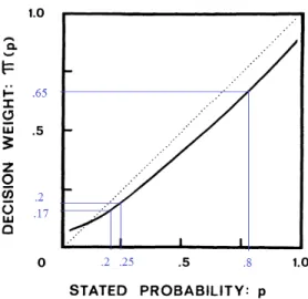
Figure 1: Kahneman and Tversky’s 1979 Weighting Function (modified) and the Certainty Effect
certainty effect. In prospect theory, ‘the certainty of $3000 80% chance of winning $4000’ is equivalent to u($3000) > .65u($4000) and ‘25% chance of winning $3000 ≺ 20% chance of winning $4000’ to .2u($3000) < .17u($4000). This is one instance of how prospect theory can formalize violations of the independence axiom. Note how the (1979) weighting function is normalized at the end point, i.e., π(0) = 0 and π(1) = 1, but not well-behaved near the end points 0 and 1. On Kahneman and Tversky’s (1979, p.282) account, this represents two “categorical distinction[s]”: between impossibility and uncertainty near the end point 0, i.e., within Rastier’s distal zone of (un)certainty, and between uncertainty and certainty and uncertainty near the end point 1, i.e., between Rastier’s identity zone and the other two zones of (un)certainty.
The main problem with this weighting function is that it allows to formally represent prefer-ences against first-order stochastic dominance. First-order stochastic dominance is a monotonic-ity condition under risk. Put informally, preference for first-order stochastic dominance ensures that lotteries with some chance to win some money are preferred to lotteries with less chance to win less money. Economists working in decision theory usually consider it as “a hallmark of rationality” (Wakker 2010, p.65), and its absence as “a fatal flaw sufficient to damn theories” (Bardsley et al. 2010, p130). In other words, preference for first-order stochastic dominance is the most important theoretical convention in decision theory from which economists derive value
judgments of rationality and irrationality. This is why prospect theory has a serious normative drawback from an economist’s perspective.19
Kahneman and Tversky (1979, p.274) try to bypass this problem by distinguishing two phases of decision making. The evaluation phase corresponds to the evaluation of lotteries through decision weights (i.e., with the weighting function). The edition phase corresponds to the process leading to the evaluation phase, represented as a set of psychological operations. One of these operations, the detection of dominance, “involves the scanning of offered prospects to detect dominated alternatives, which are rejected without further evaluation” (ibid, pp.274-5). This informal way of preventing a formal implication never convinced standard economists. What convinced at the same time standard economists, behavioral economists and even Tversky and Kahneman in their (1992) cumulative prospect theory is the so-called rank-dependent utility approach pioneered by economist John Quiggin (1982), for three main reasons. First, it formally modifies psychologists’ decision weights to avoid violations of first-order stochastic dominance while still accounting for empirical challenges such as the certainty effect. Second, it shares expected utility’s axioms with a weakened form of independence (see Quiggin 1982; Quiggin and Wakker 1994). Third, it allows folk-psychological explanations in terms of optimism and
pessimism, which admit normative interpretations (see Diecidue and Wakker 2001).20
The main distinction between standard models with rank-dependent utility and cumulative prospect theory is that Tversky and Kahneman (1992) use two rank-dependent weighting func-19Systematic violations of first-order stochastic dominance comes from the non-additivity of decision weights,
especially for small probabilities, e.g., π(.01) + π(.06) > π(.07), so that ‘1% chance of winning $10, 6% chance of winning $10 and 97% chance of winning nothing’ can be preferred to ‘7% chance of winning $11 and 97 chance of winning nothing’ (for more detailed explanations see Kahneman and Tversky themselves 1979, pp.283-4; see also Wakker 2010, sect. 5.3).
20Quiggin’s decision weights cannot be meaningfully illustrated with the certainty effect because its specificity
shows up for lotteries that have at least three non-null consequences. It does not apply to consequences’ proba-bilities, but to ranks, i.e., to cumulative probabilities. Hence consequences need to be ranked, i.e., the subscripts of the xs are meaningful, e.g., x1 ≥ ... ≥ xn. Decision weights for a given consequence are derived from the
entire probability distribution of consequences. More precisely, they are derived from the ranks of consequences
xi, which are the probability of receiving a given consequence or anything better, i.e., the cumulative proba-bility pi+ ... + pn, not just pi. Take the lottery (borrowed from Wakker 2010, pp.158-9) where you have 16
chance of winning $80, 12 chance of winning $30, 13 chance of winning $20, i.e., X = (x1, p1; x2,p2; x3, p3) =
($80,16; $30,12; $20,13). There are four ranks: 0, 16,23 and 1, corresponding respectively to the cumulative proba-bilities of more than $80 (0), $30 (0 +16), $20 (0 +16+12) and $0 (0 +16+12+13). Probabilities of individual conse-quences can be expressed in terms of differences between ranks: the probability of ‘winning $80’ is16which is equal to the rank of winning more than $30 (16) minus the rank of winning more than $80 (0); by the same reasoning, the probability of ‘winning $30’ is12 (i.e.,23−1
6) and the probability of ‘winning $20’ is 1
3 (i.e., 1 − 2
3). Finally, the
de-cision weight wiof a consequence xiis the difference between ranks transformed by a weighting function π(.) such
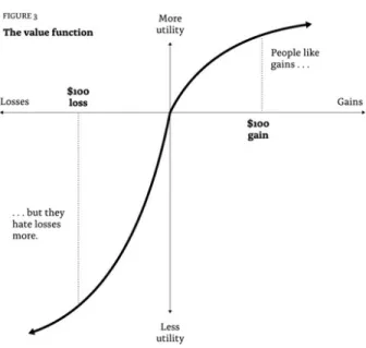
Figure 2: Prospect Theory’s Value Function from Thaler (2015, fig.3)
tions (i.e., extending Quiggin’s original approach) for gains and losses. Hence it avoids the normatively unpleasant violations of stochastic dominance while explaining more empirical phe-nomena than both standard rank-dependent models and original prospect theory (see Fennema and Wakker 1997; or Wakker 2010 appendix 9.8 for comparisons). The distinction between gains and losses is indeed central in behavioral economics and underlies its main conflicts with standard economics. If rank-dependent utility makes a step towards psychologists’ probabilistic sensitivity, it does not adopt Kahneman and Tversky’s specific perspective on consequences. Both the original (1979) and cumulative (1992) prospect theory make an explicit and central distinction between gains and losses by using the same value function u(.). It has a specific and empirically-motivated functional form that is pedagogically illustrated by Thaler (2015, fig.3); see Figure 2.
This function allows to represent reference-dependent preferences by including a reference
point where the two axes cross. Its curvature is S-shaped around the reference point so that
utility is concave for gains, convex for losses, and asymmetrically so to represent loss aversion: a difference in magnitude between utility from gains and disutility from losses (represented by the different lengths of the dotted lines). Interpreting the reference point as zero or as a given endowment allows prospect theory to account straightforwardly for various sign effects.
Reference-dependence allows to represent consequences taken as gains or losses with respect to a reference point: u(x) or u(−x). Standard economists’ way of dealing with asymmetries between gains and losses (with either expected utility or rank-dependent utility models) through asset
integration is less straightforward. It consists in representing consequences on the decision maker’s final wealth through its initial wealth w, not consequences per se: u(w + x) or u(w − x). The most salient clash between these two approaches arises with respect to a quantitative challenge, the so-called Rabin paradox. Behavioral economists Matthew Rabin (2000) considers the following preference:
nothing 50% chance of winning $110 and 50% chance of losing $100
Through some algebraic manipulations, he shows that absurd quantitative measures of risk aversion are implied by expected utility with asset integration, regardless of both initial wealth levels (and functional forms except for concavity, i.e., risk aversion). In particular, the previous preference for nothing implies the following one:
nothing 50% chance of losing $1000 and 50% chance of winning any sum of money
In short, plausible risk aversion over win/lose small stakes imply implausible risk aversion over large ones (e.g., replace ‘any sum of money’ by $1.000.000). Rabin’s solution through prospect theory’s loss aversion raise at least three interrelated issues worth discussing here.21
First, as for probability weighting, loss aversion is not necessarily irrational if a decision maker consciously puts twice more weights on losses than on gains (Wakker 2010, p.239). This underlies the most frequent criticism of prospect theory: there is only sporadic considerations but no systematic theory of how the reference point changes, which has to be guessed in a pragmatic way by decision theorists (see, e.g., Wilkinson and Klaes 2012, p.190; Wakker, 2010, p.241-2 and sect.8.7; Stommel 2013). Thus, there is a lack of systematicity not only about the 21Rabin’s results come from the whole of risk attitudes being derived from the marginal utility of consequences
in expected utility, i.e., from economists’ lack of probabilistic sensitivity. For more on the Rabin paradox, see Rabin and Thaler (2001), Barberis, Huang and Thaler (2006); Wakker (2010, pp.244-5) discusses most of standard economists’ reactions to the paradox. There is a tradition in standard economics (esp. in experimental economics) to model expected utility over income rather than over final wealth. Many responses to the Rabin paradox use this strategy but without remarking that this is tantamount to reference-dependence (see Harrison, Lau and Rutström’s 2007 appendix; and Wakker 2010, p.245). Because Rabin’s solution is through loss aversion which entails reference-dependence, the only remaining disagreement between users of expected utility over income and prospect theory seems to be about the (ir)rationality of decision makers.
fixation of the reference point, but also, by implication, on the underlying (ir)rationality of the behavior under analysis.
Second, one way of resolving the asset integration versus asset isolation conflict is to drop neither and, instead, to make value judgments about the content of decision makers’ preferences. This is Wakker’s position (2010, chap.8), who argues that rationality requires risk neutrality (or very weak risk aversion) over small consequences. In other words, Wakker argues against the translation of consumer sovereignty in decision under risk. In other words, he argues that the content of preferences (for or against risk) is amenable to rational criticism.
Third, the real difference between standard analysis and prospect theoretic analysis is not the notion of reference-point per se. It is rather that a reference point is fixed in standard analysis while it can change in prospect theory. Indeed, expected utility’s asset integration and prospect theory’s reference-dependence are in agreement when prospect theory’s reference point is a fixed level of initial wealth, so that there is “a unique relation between the [consequences] and the final wealth” (Wakker 2010, p.238). This unique relation is simply initial wealth plus consequences equals final wealth. It is when, for a given decision maker and a given set of choices, this unique relation is broken during the analysis by a change in reference point that both approaches disagree. In such cases, the traditional behavioral economics position of keeping the standard approach as the normative benchmark and using psychologists’ theories as positive models surfaces clearly: “traditional EU [expected utility] is, in my opinion, the hallmark of rationality, any deviation from final wealth due to reference dependence is utterly irrational” (Wakker 2010, p.245). In short, “[e]xpected utility is the right way to make decisions” (Thaler 2015, p.30).22
22Among the attempts at endogneizing changes of reference point (e.g., Schmidt 2003; Schmidt, Starmer and
Sugden 2008), Köszegi and Rabin (2006, 2007, 2009) can be mentioned as specifically relevant for the object of the paper because their account involves the three dimensions at once. Their determination of reference-point is (1) counterfactual (see e.g., 2006, fn3 p.1138), (2) temporal and (3) it uses tools from game theory (to model interpersonal relations between the selves of a decision maker). Furthermore, regarding the positive/normative issue, the determination is rational, i.e., they assume rational beliefs (i.e., rational expectation) for simplicity and often stress (esp. in the 2006 and 2007 conclusions) the inability of their models to account for some irrational behaviors demonstrated in behavioral economics (though see 2009, sect. III, where some of these irrational behaviors are seen as rational through the lenses of their model).
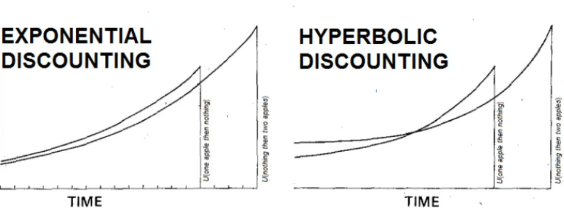
Figure 3: Exponential versus Hyperbolic Discounting and the Apple Example (modification to Ainslie 1975, fig.1)
Over time
Psychiatrist George Ainslie (1975; 1992) and his theory of hyperbolic discounting plays a role for time preferences in behavioral economics comparable to Kahneman and Tversky’s prospect theory for risk preferences. Ainslie put together a large amount of empirical observations and theoretical considerations from various disciplines on human and animal behaviors over time. He makes the case for the importance of two behavioral phenomena: impulsiveness, responsible for dynamic inconsistencies and impulse control, i.e., various ways by which humans and ani-mals try to avoid dynamic inconsistencies. Hence, the divide between standard and behavioral economics in the dimension of time is primarily marked by the distinction between impatience and impulsivity.
Figure 3 illustrates this with Thaler’s (1981) apple example. Intertemporal preference reversals, i.e., dynamic inconsistencies, are impossible under exponential discounting because the rate of discounting, i.e., the degree of impatience, is constant. Hence, a choice for ‘one apple early and then nothing’ should imply that its utility is always superior to the utility of ‘nothing and then two apples later’. This contradicts the outcome of Thaler’s example. Under hyperbolic discounting, however, the utility of ‘nothing and then two apples later’ is superior to the utility of ‘one apple early and then nothing’ at early evaluation times, before smoothly reversing as the time of getting the early apple gets closer. The closer evaluation time from the occurrence of the
consequence, the greater the rate of discounting. Hence the rate of discounting is non-constant. Ainslie interprets this as impatience and impulsiveness.
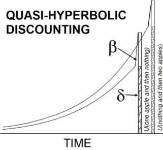
The most famous introduction of Ainslie’s work in economics was made by behavioral economist David Laibson (1994; 1997) in his models of quasi-hyperbolic discounting. His models bring together hyperbolic and exponential discounting, at least to some extents. The quasi-hyperbolic discount function in Laibson’s models is a step function. It discounts the utility of a plan as its exponentially discounted utility with an additional discounting parameter β. This parameter is (i) necessarily equal to one at the time of evaluation and (ii) can then take any value between zero and one to multiply all exponentially discounted subutilities. Formally, quasi-hyperbolic discounting is represented by Ut(X) = u(x
t) + β
∞
P
i=1
δiu(x
t+i). It is easy to see
that if β = 1, then quasi-hyperbolic discounting reduces to exponential discounting and implies dynamic consistency. It is also easy to see that if β = 0, then the decision maker does not care at all about Later and The Future in the sense that all consequences after the date of evaluation contribute nothing to the utility of a plan under evaluation. In this case the utility of a plan is just the subutility of its Instantaneous consequence. In-between, i.e., for 0 < β < 1, the closer β gets to 0, the greater the evaluation of a plan is biased by the Present consequence (with respect to an evaluation under exponential discounting). Hence the two alternative labels for quasi-hyperbolic preferences in the literature, present-biased preferences and β-δ preferences. Like hyperbolic discounting, quasi-hyperbolic discounting can imply the preference reversals un-derlying dynamic inconsistency. Unlike hyperbolic discounting, the reversal is not smooth with quasi-hyperbolic discounting. Before the time of evaluation coincides with the occurrence of consequences, quasi-hyperbolic discounting is like exponential discounting but ‘restrained’, as it were, by β < 1. When the time of evaluation coincides with the occurrence of consequences, then β = 1, which suddenly makes their utility higher, especially compared to the utility of consequences occurring later.
Figure 4 provides a graphical representation of this explanation. If time is discrete, then kinks due to β suddenly becoming equal to 1 represent the beginning of the evaluation period