HAL Id: hal-02887201
https://hal.archives-ouvertes.fr/hal-02887201
Submitted on 2 Jul 2020
HAL is a multi-disciplinary open access
archive for the deposit and dissemination of
sci-entific research documents, whether they are
pub-lished or not. The documents may come from
teaching and research institutions in France or
abroad, or from public or private research centers.
L’archive ouverte pluridisciplinaire HAL, est
destinée au dépôt et à la diffusion de documents
scientifiques de niveau recherche, publiés ou non,
émanant des établissements d’enseignement et de
recherche français ou étrangers, des laboratoires
publics ou privés.
A. Gualandi, J.-P. Avouac, S. Michel, Davide Faranda
To cite this version:
A. Gualandi, J.-P. Avouac, S. Michel, Davide Faranda. The predictable chaos of slow earthquakes.
Science Advances , American Association for the Advancement of Science (AAAS), 2020, 6 (27),
pp.eaaz5548. �10.1126/sciadv.aaz5548�. �hal-02887201�
G E O P H Y S I C S
The predictable chaos of slow earthquakes
A. Gualandi1*, J.-P. Avouac1, S. Michel2, D. Faranda3,4
Slow earthquakes, like regular earthquakes, result from unstable frictional slip. They produce little slip and can therefore repeat frequently. We assess their predictability using the slip history of the Cascadia subduction between 2007 and 2017, during which slow earthquakes have repeatedly ruptured multiple segments. We characterize the system dynamics using embedding theory and extreme value theory. The analysis reveals a low-dimensional (<5) nonlinear chaotic system rather than a stochastic system. We calculate properties of the underlying attractor like its correlation and instantaneous dimension, instantaneous persistence, and metric entropy. We infer that the system has a predictability horizon of the order of days weeks. For the better resolved segments, the onset of large slip events can be correctly forecasted by high values of the instantaneous dimension. Longer-term deter-ministic prediction seems intrinsically impossible. Regular earthquakes might similarly be predictable but with a limited predictable horizon of the order of their durations.
INTRODUCTION
There are typically two ways to forecast earthquakes. The first one considers that earthquakes result from a stochastic process: Mainshock interevent times are assumed to follow a specific distribution. This distribution is typically Poissonian and stationary (1), but it can be nonstationary if we consider a variable stress history (2) or it can be based on some renewal time model mimicking the elastic rebound theory (3). The probability of the next large event in a given time window can be estimated on the basis of the past seismicity using a probabilistic approach. The second way hypothesizes a deterministic process, for example assuming that earthquakes result from stick-slip frictional sliding as observed in laboratory friction experiments (4). The deterministic predictability of earthquakes is a matter of debate. Friction is a nonlinear phenomenon (5) and hence can result in deterministic chaos (6) with only limited predictability. Which of these two approaches is more relevant boils down to the interpretation of earthquakes as a stochastic process or as a deterministic chaotic process (i.e., a process governed by deterministic laws but highly sensitive to initial conditions). Theoretical studies and numerical simulations based on deterministic equations suggest that stick-slip sliding can be chaotic (7–11). However, we do not know whether natural earthquakes result from deterministic chaos, and, if so, what would be their predictability horizon. Detecting chaotic behavior in geophysical time series is a difficult task, mainly because of the short and noisy data generally available (12). While historical catalogs (13) or particular earthquake sequences (14) have been used to argue for chaos, characterizing the chaotic behavior of regular earthquakes has been a challenge because of the short observation time period, making it difficult to record multiple ruptures of a same fault segment. This limitation does not apply to laboratory earthquakes and slow earth-quakes, slip events that produce very little slip at slow rates and radiate very little seismic waves (15).
Recent laboratory experiments have shown that both slow and fast ruptures are preceded by crackling that can be detected and used to forecast the time of failure, implying that the stick-slip behavior
observed in these experiments is governed by some deterministic dynamics (16). In nature, a possible chaotic behavior has been inferred in the particular case of low-frequency earthquakes (17), a class of small slow earthquakes that can be detected and characterized with seismology. Geodetic position time series capture the whole deformation independently of radiated seismic waves and can thus give a more comprehensive view of fault slip, in particular during slow earthquakes. Here, we focus on slow slip events (SSEs) imaged from geodetic time series. SSEs are a stick-slip phenomenon, which presents a recurrence time much shorter than that of typical earth-quakes, of the order of months or years instead of decades or centuries. They have been documented along major subduction megathrusts (15), reaching moment magnitudes [Mw] comparable to that of large earthquakes [Mw > 7]. SSEs are notably similar to regular earth-quakes. They evolve into large pulse-like ruptures (18). They follow similar scaling laws and exhibit systematic along-strike segmentation (18–19). These characteristics make them a most suitable system to study the dynamics of frictional sliding at scale of the order of hundreds or thousands of kilometers. Our goal is to characterize whether the observed slip time series irregular behavior is emerging from an underlying deterministic dynamics or from a stochastic nature of the source.
RESULTS
We focus on the Cascadia subduction using the slip history on the megathrust derived from the inversion of geodetic records over more than 10 years, from 2007.0 to 2017.632 (20). SSEs in Cascadia show a first-order segmentation consisting of 13 major segments, which produced repeating ruptures over the studied time period (18) (Fig. 1). We low-pass filter the slip time series to calculate the slip rate, and then integrate it over the area of a given segment to obtain the slip potency rate time series for all the 13 segments
[ P ̇ s (t ) , s = 1, … , 13 ; Fig. 2, figs. S1 to S7, and the “Slip potency rate”
and “Filters” sections]. The results shown here were obtained using the filter adopted by (20), i.e., an equiripple filter (EF) with normalized passband and stopband frequencies of 35−1 and 21−1 ( EF 1/211/35 ) , pass-band ripple of 1 dB, and stoppass-band attenuation of 60 dB. The type and characteristics of the filter have a limited influence on our results (“Filters” and “Surrogate data” sections). We resort to the embed-ding theory (ET) (21) and the extreme value theory (EVT) (22) to
1California Institute of Technology, Pasadena, CA, USA. 2Laboratoire de Géologie,
Département de Géosciences, École Normale Supérieure, PSL University, UMR CNRS 8538, Paris, France. 3LSCE-IPSL, CEA Saclay l'Orme des Merisiers, CNRS UMR 8212
CEA-CNRS-UVSQ, Université Paris-Saclay, 91191 Gif-sur-Yvette, France. 4London
Mathematical Laboratory, London, UK.
*Corresponding author. Email: adriano.geolandi@gmail.com
Copyright © 2020 The Authors, some rights reserved; exclusive licensee American Association for the Advancement of Science. No claim to original U.S. Government Works. Distributed under a Creative Commons Attribution NonCommercial License 4.0 (CC BY-NC). on July 2, 2020 http://advances.sciencemag.org/ Downloaded from
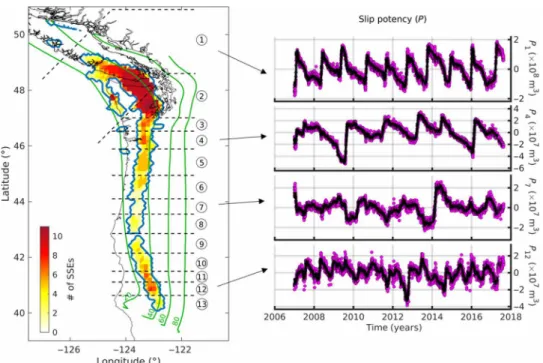
Fig. 1. SSEs in Cascadia. Left: Modified from (18). Blue contour line: SSE region. Color palette: Number of times a specific segment has ruptured in the time interval (2007.0, 2017.632) following the available SSE catalog (20). Dashed black lines indicate the segmentation from (18), here adopted. Black continuous line shows the coast for reference. Green lines are isodepths in kilometers. Right: Slip potency [P(t)] for four selected segments. The calculation is performed over the entire area belonging to the segment and colored in the left panel. Magenta dots: Slip potency for segments #1, #4, #7, and #12. Black dots: Causal low-pass–filtered slip potency. The causal filter introduces a 115-day time delay. For visual purpose, the filtered time series is shifted back to the starting date 2007.0 (see “Filter” section for more details).
Fig. 2. Slip potency and slip potency rate. (A) Causally filtered slip potency (black dots) for segment #1 (same as in Fig. 1). Red dashed lines indicate the epochs for which the instantaneous dimension d is larger than its 95th quantile up to that epoch and for which the slip potency is smaller than its 50th quantile up to that epoch. (B) Slip potency rate (black dots) for segment #1, calculated as the derivative of the causally filtered slip potency (A) using a 1-day interval time step, plus the long-term slip potency rate. Red dashed lines as in (A).
on July 2, 2020
http://advances.sciencemag.org/
study the dynamics of the system (see Methods). The system that we study is limited to the slow slipping belt on the megathrust, at a depth of about 30 to 40 km (Fig. 1). We treat it as an isolated dynam-ical system, thus neglecting the potential interactions with other parts either of the megathrust or of the surrounding medium. Since we are focusing on the slow slipping region, it follows that we are dealing with only a part of the whole phase space. The phase space is that space where all possible states of the system can be represented, i.e., that space having for axes all the variables needed to explain the dy-namics of the system. Because of the assumption of isolated system, we refer to the region representing the slow slipping phenomenon as the phase space, and to the trajectories in it, which represent how the state of the dynamical system evolves with time, as the attractor of the system. The slip rate (and thus the slip potency rate, which is directly proportional to it) is considered to be the main observ-able variobserv-able governing the evolution of friction in laboratory exper-iments (5). To apply ET and EVT, we need the temporal evolution of at least one of the variables needed to explain the system’s dynamics, and the slip potency rate is therefore a good candidate. It shows episodic bursts with the most extreme events occurring quite regu-larly (Fig. 2 and figs. S1 to S7).
A quantity of interest to characterize a dynamical system is its dimension, a geometrical property of the underlying attractor. There are multiple definitions of an attractor’s dimension, but they should agree in telling how many effective degrees of freedom (dof) are needed to explain the dynamical system (23). The ET methods indicate an embedding dimension m ≃ 10 for all the segments, consisting in a correlation dimension of the attractor ≲ 5 (figs. S8 to S12 and “Embedding theory” section). The application of EVT for the calcu-lation of the average attractor dimension (D) (see “Extreme value theory” section) confirms low average dimension, for which we get a value <4 for all the segments (3.1 < D < 3.5; green dots in Fig. 3). However, the signal-to-noise ratio (SNR) is high enough only for segments located in the northern section of the megathrust (seg-ments #1 and #2). This is evident when surrogate data (24) are used to test the significance of the observed low dimensionality of the system (Fig. 3, “Surrogate data” section, and figs. S13 and S14).
The dimension, D, being an average in the phase space, does not capture the information about transient instabilities. Recent advances in EVT applied to dynamical systems theory have proven that it is possible to characterize these transient instabilities via two instantaneous properties (25): the instantaneous dimension (d) and the instanta-neous extremal index (). These quantities refer to the state of the system in a given location of the phase space and, for this reason, are also referred as local. As in (25), here we name them “instantaneous,” because they depend on the specific time, and we want to avoid con-fusion with “local” in a geographical sense. Their distribution and temporal evolution are shown in figs. S15 to S19. The instantaneous dimension, d, indicates the number of variables needed to explain the dynamics of the system in a specific phase space location. We expect to find high values of d when a metastable state is approached. In this situation, the segment is transitioning from a stable to an unstable regime, or vice versa, and more variables are then needed to explain the state of the system. This is apparent from Fig. 4A, where a section of the attractor is plotted with d color coded, with high values of d marking the onset and end of large SSEs.
The instantaneous extremal index () measures the inverse of the average persistence time around a given state in a region of the phase space (Fig. 4B). In this sense, it is a local and instantaneous
quantity. The extremal index (), a parameter in the range [0,1], measures the degree of clustering of extremes in a stationary process
[ P ̇ s (t) in our case] and can be defined as the reciprocal of the mean cluster size (26). A relationship between and the metric entropy
H of a system has been recently demonstrated (27)
~1 − e −H (1)
The relationship between and is not as straightforward as the one between D and d, but we must have ∈ [min, max]. We can, thus, deduce a range of values for H. Given the values of that we have found (figs. S15 to S19) and the fact that the metric entropy is equal to the sum of all the positive Lyapunov exponents, we deduce that there is at least one positive Lyapunov exponent in our system. The positive Lyapunov exponents tell us how rapidly two trajectories in the phase space exponentially diverge. We can thus derive a pre-dictability time t* as the inverse of the metric entropy, and we find
t* ranging from a few days to about 2 months (Table 1). A similar
conclusion, with predictability horizons of the order of days to weeks, is reached by applying nonlinear forecasting analysis (NFA) tech-niques (based on ET, see Methods) to estimate H (figs. S20 and S21) (28–29). The NFA provides only a lower bound estimate of H (29). It follows that the NFA estimate of t* is an upper bound, which, for all the segments, is in the range estimated from EVT (Table 1). DISCUSSION
According to the EVT, the dynamics revealed by the filtered data requires at least four variables, which is the first integer above the fractal value of D. The description of stick-slip friction in the laboratory can be schematized by a spring-slider system and, in a fully inertial model, must involve slip, slip rate, and at least one additional “state” variable to allow fault healing after slip events so that they can repeat. The underlying physics and the number of state variables needed to explain laboratory friction remain matters of debate (30). It is im-portant to clarify here the difference between the state variables coming from the rate-and-state description of friction (RS-state variables) and the state variables that determine the state of the system. Typically, a point in the phase space is defined by a state vector, with elements given by the variables needed to explain the dynamics of the system. An RS-state variable is only one among all the state variables belonging to a state vector.
In the absence of coupling with other spring-slider systems, the expected number of dof is 2 (because the system is described by a second-order differential equation) plus the number of RS-state variables, and the dimension should be between dof-1 and dof. For a noninertial single spring-slider, adding a second RS-state variable is a viable way to enact chaotic behavior, and a Kaplan-Yorke dimension of 2.119 ± 0.001 has been derived (8), consistent with the fact that we can drop 1 dof because of the noninertial assumption. A one- dimensional, fluid-infiltrated, rate-and-state friction spring-slider has 5 dof, i.e., its dynamics can be described by five variables: load-ing shear stress (which is proportional to slip in case of constant loading rate), slip rate, one RS-state variable (potentially related to the effective contact area) (31), porosity, and pore pressure (32). To describe SSEs, we can assume a quasi-static condition, and under this hypothesis, the number of state variables drops to four, consistent with the number of dof recovered from our analysis in Cascadia where pressurized fluid has been invoked to justify SSEs’ existence (33).
on July 2, 2020
http://advances.sciencemag.org/
Fig. 3. Surrogate data test. The average attractor dimension D has been estimated as the average of the instantaneous dimension d. The surrogate data have been obtained randomizing the phases of the Fourier-transformed slip potency and maintaining correlation between patches (see the “Surrogate data” section). The p-value is estimated after calculating D for every surrogate and comparing the data derived D with the distribution of the surrogate data derived Dsurrogate. Only segments
#1 and #2 show an average dimension significantly (p < 0.001) lower than the one derived from the surrogate data independently from the choice of the filter, of the norm to calculate distances, and of the quantile threshold to determine the exceedances (see “Extreme value theory” section and figs. S13, S14, and S22 to S25).
Fig. 4. Instantaneous dimension and instantaneous extremal index on a section of the attractor. We use the slip potency [P(t)] and the slip potency rate [ P ̇ (t ) ] as variables to reconstruct a section of the attractor. The color palette indicates the instantaneous dimension d and the instantaneous extremal index in the top and bottom panels, respectively.
on July 2, 2020
http://advances.sciencemag.org/
In a coupled system, the loading term would also depend on the variables associated with neighboring fault segments, which need to be introduced in the state vector to describe the system’s evolution. In the case of a one-dimensional system, similar to the one observed in Cascadia with along-strike segmentation, we would expect dimensions as high as 12, with the extra 8 dof carried in by the two adjacent segments. The neighbors’ effect may be particularly relevant in starting or stopping a slipping event. The maximum retrieved instantaneous dimension is in the range between 11 and 18 for the segments with high SNR. Considering the first-order segmentation here adopted and the available noisy data, we consider this result in good agreement with the maximum expected dimension of 12, as in a one-dimensional spring-and-slider chain. Potentially, an along-dip segmentation would also increase the number of neighbors, i.e., the number of dof. The proposed description considers only short-range elastic interactions, like in the Burridge-Knopoff model. Long-range interactions (i.e., interactions with segments further than the adjacent neighbors) would further increase the instantaneous dimension of the attractor.
Since the filter parameters may affect our findings, we perform the same analyses on the unfiltered time series as well as on time series filtered with various parameters and different filters. The surrogate data test on unfiltered time series suggests that we cannot reject the null hypothesis for which data can be described via a linear stochastic model (fig. S22). Furthermore, for unfiltered time series, we find extremal index values close to 1, with predictability horizons smaller than the data sampling rate, indicating a random system (fig. S26 for an example relative to segment #1). A similar conclusion would be reached by ET-based techniques (figs. S20, S21, and S27). This shows that, if not filtered, the noise in the data is dominating, masking the SSE dynamical structure. A more detailed discussion of the filter effects (and the tested filters) is reported in
the “Filter” and “Surrogate data” sections. We stress here that filters applied to pure noise can potentially produce the spurious identifi-cation of finite correlation dimension (34), and for this reason, we further test the effects of the filters on the predictability of the time series generating (pseudo-)random time series and applying the same filters to them. The number of generated random time series is equal to the number of subfaults in segment #1, which is the segment with the largest number of subfaults. We then generate surrogate data and calculate the average dimension on both the filtered random time series and the surrogate data. The result shows that we would not be able to reject the null hypothesis according to which the time series were generated by a random process (fig. S28). We thus consider unlikely that the filters here adopted are introduc-ing an apparent chaotic dynamics, and we notice that, for the cases that pass the surrogate data test, D is typically between 3 and 4 for all segments, independently of the chosen filter parameters (figs. S22 and S23).
Not all segments pass the surrogate data test. We conclude that SSEs on the northernmost segments of the Cascadia subduction zone (segments #1 and #2) result from deterministic chaos, while the central part (segments #3 to #5) shows ambiguous results, and for the southernmost portion of the fault (segments #6 to #13), we cannot infer deterministic chaos with the data at our disposal (figs. S13, S14, and S22 to S25). Our analysis implies that it should be possible to forecast the onset of large SSE ahead of time based on an explicit deterministic representation of the system dynamics or some machine learning algorithm that would implicitly capture it. Along that line, it is notable that the increase in instantaneous dimensionality seems to constitute a reliable precursor of the large SSEs (segments #1 and #2; Fig. 2 and fig. S1). The causal filter adopted here introduces a group delay larger than the predictability horizon time, implying that this approach cannot be used for real- time forecasting. Alternative noise reduction or forecasting techniques need to be investigated for this purpose, or more accurate data would be needed to avoid the filtering step.
In conclusion, we have shown that continuous spatiotemporal models of SSE evolution (20) provide insight into fault dynamics because, where the SNR is sufficiently high, we have shown that SSEs in Cascadia manifest chaotic dynamics. In other words, SSEs can be described as a deterministic, albeit chaotic system rather than as a random or stochastic process. The estimated predictability horizon is of the order of days or weeks that is equivalent to a fraction of the typical large SSE duration in Cascadia, which is the representative time scale of the instability. If the dynamics derived from the filtered time series is representative of the true underlying dynamics, then long-term prediction of SSEs (i.e., over a time horizon much longer than their duration) seems intrinsically impossible. This implies that for long-term predictions, a stochastic approach remains the best tool at our disposal, while short-term deterministic predictions should be achievable. As SSEs might be regarded as earthquakes in slow motion (18), regular earthquakes might be similarly chaotic and predictable. If the relation between predict-ability horizon and event duration holds also for regular earthquakes, then this would imply that long-term predictions of earthquakes are intrinsically impossible, and the predictable horizon would be only a fraction of the regular earthquakes’ typical duration (10 to 100 s for Mw > 6 earthquakes). Furthermore, it might be possible to augment the capabilities of early warning systems with a forecast of the final magnitude while the event is still ongoing.
Table 1. Predictability horizon. Predictability horizon t * = 1_
H for all
segments for causally filtered time series with EF 1/351/21 . The upper bound estimated via EVT is lowered by the upper bound estimated via NFA.
Segment EVT NFA
# t min* (days) t max * (days) t Eq.15 * (days) t Eq.16 * (days) #1 3.5 65.0 17 ± 3 9.6 ± 2.3 #2 2.8 34.7 15.0 ± 1.8 7.5 ± 0.9 #3 3.1 34.2 19.8 ± 2.9 9.8 ± 1.5 #4 2.6 32.3 20.3 ± 2.9 10.0 ± 1.4 #5 2.9 29.7 18 ± 3 8.8 ± 1.7 #6 2.5 62.1 14.1 ± 1.4 7.1 ± 0.7 #7 2.8 50.7 19 ± 3 9.4 ± 1.5 #8 2.8 26.9 17.4 ± 2.2 8.8 ± 1.1 #9 2.4 26.3 16.3 ± 1.7 8.2 ± 0.9 #10 2.6 29.8 13.5 ± 1.1 6.7 ± 0.5 #11 2.3 22.5 15.1 ± 1.9 7.5 ± 0.9 #12 2.2 22.6 17.4 ± 2.6 8.6 ± 1.3 #13 2.7 31.3 25 ± 7 12 ± 3 on July 2, 2020 http://advances.sciencemag.org/ Downloaded from
METHODS
Slip potency rate
Given a subfault (n) of a given segment (s = 1, …,13), we apply a low-pass filter to the slip history [ u snrough (t ) ] from (20) to obtain a smoothed slip history [usn(t)]. Since chaotic systems are extremely sensitive to initial conditions, we test several low-pass filters (details are provided in the “Filters” section). We then multiply the smoothed slip history by the area of each subfault (Asn), getting the slip potency for each subfault
p sn (t ) = A sn u sn (t) (2) The total slip potency for the s-th segment is calculated as the slip potency integral over the entire slipping area. In a discretized case where there are Ns subfaults belonging to the s-th segment, the total slip potency is calculated as
P s (t ) = ∑ n=1 N s
A sn u sn (t) (3) We also construct slip potency rate curves for each subfault
p ̇ sn (t ) = A sn ( v 0sn + u ̇ sn (t ) ) (4) and the total slip potency rate for each segment
P ̇ s (t ) = ∑ n=1 N s
A sn ( v 0sn + u ̇ sn (t ) ) (5) where v0sn is the long-term reference loading velocity for a given patch belonging to a specific segment as derived from (20).
The choice of the variable to use for the dynamics reconstruction is important because it can bias the correlation dimension estima-tion. In particular, the correlation dimension can be lowered when using a variable strongly correlated only with a few variables of the system (35). Having in mind the rate-and-state formalism for friction (5), we hypothesize that the slip rate, and thus the slip potency rate, is not only more strongly coupled than the slip potency to the other variables of the system, but it is also coupled with more variables (e.g., the state variables). We find smaller values for the correlation dimension of the attractor when using the slip potency as observable (figs. S8 to S12 and S29 to S33 and “Embedding theory” section), confirming our intuition that slip potency rate is a more suitable observable.
Filters
The effect of low-pass filters on dynamical systems’ dimension estimation has been extensively studied. Ideal linear low-pass filters introduce further equations in the dynamical system, leading to an increase in dimensionality (36). Finite order nonrecursive filters instead do not modify quantities estimated via ET, but this is not strictly proven for practical cases where finite time series are avail-able (37). Proper low-pass filtering data can improve the dynamical system characterization (38), and we thus restrain ourselves to finite order nonrecursive filters, which implies that the filtered value
usn(t) is obtained from the current and past Nb nonfiltered values, u snrough , according to
u sn (t ) = ∑ i=0 N b
b i u snrough (t − idt) (6)
where dt is the data sampling rate, i.e., 1 day. First, we test an EF with fixed passband ripple and stopband attenuation of 1 and 60 dB, respec-tively, and we test 10 combinations of normalized stopband and passband frequencies:
{
f ipassband}
10 i=1 = [7(2 + i ) ] −1 and{
f istopband}
i=110 = (7i) −1 . We follow the MATLAB notation for which the normalized fre-quency is unitary when it is equal to the Nyquist frefre-quency. The filters are designed using the built-in function designfilt, from which we extract the corresponding transfer function coefficients { b i } i=0 N b via the function tf. The coefficients are then used by the function filter to generate the smoothed signal usn(t). With the tested combina-tions, the order of the filter (i.e., Nb) takes the following values when increasing i: 48, 125, 230, 363, 484, 664, 871, 1106, 1368, and 1658. For each designed filter, we show the filter response in figs. S34 and S35. The results shown in the main text are those obtained using an EF and the parameters adopted in (20) to automatically pick 64 SSEs from the dataset here studied, i.e., f ipassband = 35 −1 and fi
stopband = 21 −1 . We test also a Hamming Window filter (HWF; which is a weighted moving average filter), commonly used in signal processing, which offers an easier way to tune the filter order (Nb) and its normalized frequency cutoff (fcutoff). We test both a variable fcutoff fixing Nb to 60 (i.e., we use 2 months of data before the current epoch to smooth the signal; figs. S36 and S37) and a variable Nb fixing fcutoff to 28−1 (figs. S38 and S39). In the first case, we vary
{
f icutoff}
i=1 10
= (7i) −1 , while in the second case, we vary { N b i } i=110 = 7i − 1 , i.e., we use data of epoch t and the 6 epochs before, 13 epochs before, and so on until using a total of 10 weeks of data. We use the MATLAB built-in function fir1, which adopts a normalized gain of the filter at fcutoff of −6 dB. We observe that reducing the cutoff frequency lets the underlying dynamics emerge, and we consistently observe a finite fractal di-mension significantly smaller than what would be calculated from surrogate data (fig. S22). We refer the reader to the “Surrogate data” section for more details.
All tested filters have a constant group delay (figs. S34 to S39). The information on the group delay is relevant when discussing about the predictability horizon of the system (see Discussion). The effects of the EF filters on the time series are shown in figs. S40 to S44. For readability, the filtered time series have been shifted back in time of the corresponding group delay to be in phase with the original time series. To test whether there is any difference between causally and noncausally filtered time series, for the filter EF 1/351/21 , we also construct a noncausal filter, knowing that noncausal filters cannot be adopted for real-time applications, because they use information from future epochs. We use the function FiltFiltM (https://www. mathworks.com/matlabcentral/fileexchange/32261-filterm) to generate zero-phase shift (i.e., noncausal) filtered time series, and we find similar results to those obtained with a causal filter (figs. S13, S26, and S28). In all tested cases, we retrieve similar average dimensions, lower than those determined from nonfiltered time series (fig. S45). The application of a low-pass filter reduces the dimensionality of the system from values typically >6 to values <4.
Embedding theory
We apply two methodologies based on ET to determine the correlation dimension of the strange attractor, and the NFA, also based on ET, to estimate the metric entropy associated with the time series.
The correlation dimension is defined as (39)
on July 2, 2020
http://advances.sciencemag.org/
= lim r→0 lim T→∞
Log(C(r, T ) )
─
Log(r) (7)
where C(r, T) is the correlation integral, r is a variable threshold distance,
T is the time series length, and we use the base-10 logarithm Log.
The construction of the correlation integral typically involves two parameters: the delay time () and the embedding dimension (m). Given a scalar time series x(t), for example P ̇ s (t) , its values are used to construct an m-dimensional vector delaying in time the time series of an amount for m − 1 times
F(t, τ, m ) = [x(t ) , x(t − τ ) , … , x(t − (m − 1 ) τ ) ] (8) We can now define the correlation integral as (40)
C(r, T, w ) = 2 ─ T 2 ∑ t 2 =w T ∑ t 1 =1 T− t 2 H(r − ‖F( t 1 + t 2 , τ, m ) − F( t 1 , τ, m ) ‖) (9) where we introduce a cutoff parameter w > 1 to improve the convergence of the classical algorithm (w = 1) toward its limit T → ∞, and H is the Heaviside function. Values of w~corr are recommended, where corr is the autocorrelation time for the specific scalar time series under examination (40). We calculate corr using the batch means method (41).
Basically, the algorithm counts how many m-dimensional vectors are closer than r at different times. If m ≥ 2 + 1, then F is an embedding function of the strange attractor (42), and we expect the correlation dimension to be independent of m. Figures S8 to S12 and S29 to S33 show the versus Log(r) curves for different m. The selected delay times are chosen to emphasize the scaling region. For every segment, we have tested values of = 2i + 1 days, with i from 1 to 6, and m = 4j, with j from 1 to 5. In the case of a stochastic signal, we might expect that a scaling relationship between C(r) and
r does not hold, and larger values of are calculated when increasing m, i.e., does not saturate. Nonetheless, autocorrelated noise in short
time series can fool the described algorithm (24). For this reason, surrogate data are typically introduced, but instead of evaluating the plateau for , which is quite subjective, we prefer to apply the methodology from EVT for this calculation. Given the time delays retrieved from ET (see figs. S8 to S12), one accurate slip rate data per week might be sufficient to reconstruct an embedding for SSEs.
The second methodology derived from ET needs only the definition of the delay time to determine the minimum embedding dimension (43). The algorithm still uses the embedding function F, but it exploits the nearest neighbors counting in the reconstructed phase space to detect false neighbors when changing the embedding dimension m.
The following two quantities are defined E(m ) = 1 ─ T − mτ ∑ t=1 T−mτ ‖F(t, τ, m + 1 ) − F n(t,m) (t, τ, m + 1 ) ‖ ──────────────────── ‖F(t, τ, m ) − F n(t,m) (t, τ, m ) ‖ (10) E * (m ) = 1 ─ T − m ∑ t=1 T−m ‖x(t + m ) − x n(t,m) (t + m ) ‖ (11) where 1 ≤ n(t, m) ≤ T − m is an integer such that Fn(t, m)(t, , m) is the nearest neighbor of F(t, , m). From these two quantities, the ratio at two subsequent embedding dimensions is calculated
E 1 (m ) = E(m + 1) ─E(m) (12) E 2 (m ) = E * (m + 1) ─ E * (m) (13)
The quantity E1 is relevant because if the studied time series is the result of a dynamic process, i.e., it comes from an attractor, then
E1(m) saturates (43). In other words, we reach a value m such that Eˆ 1 stops changing increasing m above ˆ m . The minimum embedding
dimension will then be m + 1 . The second quantity, Eˆ 2, is intro-duced to check for randomness in the data. In theory, for stochastic time series, E1 should never saturate, but in practical cases, it can be unclear whether E1 is slowly increasing with increasing m or not. If the time series of interest is the result of a stochastic process, then we expect future data points to be independent from the previous ones. This means that E2(m) = 1 for each m. If the studied time series is instead the result of a deterministic process, then
E2 is not constant, and there must exist some m values such that
E2(m) ≠ 1.
We show in fig. S27 the results on both causally filtered (i.e., present values depend only on the past and the present, such that the statistic E2 can be used) with EF 1/351/21 and nonfiltered time series for the example of segment #1. A minimum embedding dimension
m ≃ 10 is detected from filtered data, implying a correlation dimension
≤ (m − 1)/2 ≲ 4.5, while for nonfiltered data, E2 remains almost constant at unitary values. This result is consistent with the results from EVT, for which a close to 1 is calculated for the nonfiltered time series (e.g., fig. S26).
Another quantity of interest to characterize a chaotic system is its metric entropy H. NFA also works using nearest neighbors in the phase space, and it is a powerful approach not only to estimate H from the short time series but also to assess the chaotic or stochastic nature of the time series under study (28–29). We apply here a first-order NFA approach (28). Being based on ET, we first embed a time series in a phase space of dimension m using delay coordinates with delay time . The idea then is to use the first half of the time series (training set) to learn a nonlinear map to make a prediction
Tp time steps in the future using a local linear approximation in the phase space. We then use the second half of the data (test set) to test the learned prediction and assess the chaoticity of the time series. In practice, the following are the steps of the procedure:
1) Embed the time series x(t) like in Eq. 8 to create the obser-vation F(t, , m) at time t.
2) For a given point in the test set F(t, , m), find the k nearest neighbors { F n (t, τ, m ) } n=1k belonging to the training set. [We must have at least k = m + 1, but, as recommended in (28), to ensure stability of the solution, it is better to take k > m + 1. Here, we use
k = 2m + 1.]
3) Use the k nearest neighbors in the training set [for which
x(t + Tp) is known] to find the best local linear predictor A. 4) Use A to predict the value of x at time t + Tp in the test set: ˆ x (t, T p ) .
5) Compare x(t + Tp) and ˆ x (t, T p ) in the test set to estimate the root mean square error (RMSE ) = 〈 [ ˆ x (t, T p ) − x(t + T p ) ] 2 〉 1/2 that we use as a measure of predictive error.
6) Normalize the prediction error by the root mean square deviation (RMSD) of the data in the test set: ϵ = _RMSE
RMSD , with RMSD = 〈[ x(t) − 〈x(t)〉]2〉1/2.
If ϵ = 0, then the prediction is perfect; if instead ϵ = 1, then the prediction is as good as a constant predictor ˆ x (t, T p ) = 〈x(t ) 〉 . For a
on July 2, 2020
http://advances.sciencemag.org/
stochastic system, we expect ϵ to be independent of Tp, while for a chaotic system, we expect ϵ to increase when increasing Tp. We have tested various embedding dimensions m and delay times , ob-taining similar results. In figs. S20 and S21, we show the results rel-ative to m = 9 (i.e., we assume an average dimension between 3 and 4 for the underlying attractor, as estimated via EVT) and = 7 days. We show the evolution of ϵ versus Tp for all the segments using the same filter adopted in (20) (fig. S20), and for segment #1 varying the filter parameters (fig. S21). The black lines indicate the value calcu-lated for the unfiltered time series, while the blue and red lines cor-respond to ϵ for the various segments or filter parameters. We find that for the unfiltered time series, ϵ ≈ 1, confirming the dominant role of stochastic noise, while for sufficiently effective filters, ϵ in-creases with Tp, as expected for a chaotic system. These graphs can be used to estimate the metric entropy H using the following equa-tion, valid in the limit ϵ ≪ 1
ϵ( T p ) ≈ C e 2H T p N −2/D (14)
where N is the number of data points and D is the (average) attrac-tor dimension (for which we use the values estimated from EVT). It follows that
f ( T p ) = ln ϵ( T p ) + 2 ─
D ln N ≈ ln C + 2H T p (15)
and C and H are estimated via least square using points for which ϵ ≤ 0.3 (green dashed line in figs. S20 and S21) to fit Eq. 15.
Another estimate of H, which does not depend on a particular forecasting technique, can be obtained using the predictions to cal-culate the rate of loss of information from the time series (29). We calculate the correlation coefficient () between ˆ x (t, T p ) and x(t +
Tp) in the testing set, which will be a function of Tp. After some approximations, the following relation can be derived (29)
ln(1 − ( T p ) ) = c + 2H T p (16) from which we can estimate c and H. The number of points to use for the estimate is not strictly defined. Previous studies have used 2 (29) or 6 (44) points for example. The resulting values of t* for all segments using the same EF adopted in the main text are reported also in Table 1.
Extreme value theory
We use recent results of EVT to overcome some of the issues en-countered when using ET algorithms. In particular, we would like (i) a method to rigorously calculate a particular statistic (for exam-ple, the attractor’s dimension) and, consequently, test whether the calculated quantity is the result of a random process or not, and (ii) a method to calculate also instantaneous properties of the attractor. The main idea behind the usage of EVT for the characterization of a dynamical system is to connect the statistics of extreme events to the Poincaré recurrence theorem (25, 45).
Let us consider a generic point on a strange attractor. The in-stantaneous dimension is a quantity that measures the density of neighbors in the phase space around . To calculate this density, we can ask ourselves the following question: What is the probability to visit again a region of the phase space close to (i.e., in an arbitrary small radius from) ? If we had access to all the possible states of the system (z), then we could calculate the distances from the actual state under study, (z, ). Then, we would like to construct a
ran-dom variable related to (z, ) and use the second theorem of EVT (46) to be able to gain information about the density of neighbors around . The second theorem of EVT states that, given a random variable Z with nonvanishing probability distribution, we can set a threshold value q such that, for q sufficiently large, values of Z that exceed q (or exceedances) follow a generalized Pareto distribution (GPD).
For real case scenarios, we might only have one scalar time series, and here, we consider the univariate case. Similarly to what is done to characterize atmospheric flows (25), we assume that our observed scalar time series (i.e., the slip potency rate) approximates possible states of the system. The only requirement to apply this methodology is the observed time series to be sampled from an underlying ergodic system. A possible improvement would be to consider a multivariate case with slip potency rates and/or slip potencies from adjacent segments, but we defer this complication to future investigations. For our case of interest, to generate the pool of all possible z, we consider the slip potency rates of all subfaults belonging to the segment under examination (Eq. 4). We then select to be equal to the slip potency rate at a certain epoch t and calcu-late the distance from all other possible states that we have recorded at different times. Recent studies (45, 47) have shown that if we con-struct the random variable given by the negative log distances, Z = − ln ((z, )), then we can use the GPD shape parameter () to cal-culate the instantaneous dimension as
d( ) = 1 ─
() (17)
This assumes that the exceedances follow a GPD. We visually inspected the Q-Q plots of the exceedances versus a GPD, and dis-crepancies between the observed quantiles and those predicted by a GPD are noticed especially in the high quantile of the distribution. This probably reflects the fact that not many extreme events have been observed and a longer slip history may provide better results. Repeating this calculation for different values of extracted from the pool of values z, we can then estimate the attractor dimension by simply averaging over d: D = 〈d()〉. This is a very powerful result for two reasons. We can calculate the attractor dimension (i) with-out the need of an embedding and (ii) simply setting one parameter: a threshold q on the negative log distances. Here, we have used q = 0.98 percentile and q = 0.99 percentile of the negative log distance, and we have tested both L-1 and L-2 norm distances. The results are overall similar (green dots in figs. S13 and S14). We can now apply the method of surrogate data to each segment and compare the re-constructed attractor dimensions with the one calculated from real data. We refer to the “Surrogate data” section for more details. We notice that using a threshold q = 0.99 reduces the average dimension to values <3. The threshold quantile q does not affect the conclusion that a chaotic deterministic dynamics can be successfully detected only for the northernmost segments. It affects though the interpreta-tion of the total number of dof needed to explain the system. Following the spring-and-slider interpretation, if 3 < D < 4, then a second RS-state variable may be needed (see Discussion). Longer time series will help to resolve this ambiguity, since the value of q = 0.99 may be too high for the amount of available data.
Another quantity of interest that can be derived is the instantaneous extremal index of the system (). In the main text, we have described the extremal index () as the reciprocal of the mean cluster size
on July 2, 2020
http://advances.sciencemag.org/
(26). The instantaneous extremal index can instead be defined as the inverse of the persistence in the phase space, where the per-sistence tells us how long the trajectory sticks in the proximity of a certain point in the phase space. In other words, while d is related to the density of points in a certain neighborhood of the phase space, i.e., how many times a certain region of the phase space is visited, the persistence time indicates for how long the system stays in a region in the neighborhood of a given state. If a state is a fixed point, then we expect an infinite persistence, i.e., null . On the other hand, if we are studying a stochastic process, then we expect the persistence to tend to 0, i.e., unitary . In other words, we expect that at a certain epoch t, the system will be in a state , and then at a subsequent epoch t + t to be in a region of the phase space far from the one occupied at time t. Looking at the extremal index from this angle gives us the intuition that it can be related to the predictability of the system. As mentioned in the main text, in a recent study (27) this connection has been made explicit (see Eq. 1).
We calculate via a maximum likelihood estimator (48). When we look at the calculated (figs. S15 to S19 for noncausal filter and fig. S26 for causal and noncausal filter relative to segment #1), we see that both causally and noncausally filtered data show values far from 1. This already indicates that, no matter the causality or not of the filter, the system at the selected frequencies shows predictability features. We observe a different situation when performing the analysis on nonfiltered data (fig. S26). The values of are now very close to 1, implying a predictability horizon shorter than the sampling time. This is consistent with the fact that, in such nonfiltered slip potency rate time series, the high-frequency noise dominates, which is a random process.
Surrogate data
The concept behind surrogate data techniques is rooted in statistical hypothesis testing. The method requires to state a null hypothesis, and, using the words in (24), “The idea is to test the original time series against the null hypothesis by checking whether the discriminat-ing statistic computed for the original time series differs significantly from the statistics computed for each of the surrogate sets.” The necessity to use surrogate data derives from the intrinsic finiteness of the available data: It is always possible to generate the observa-tions with a particular random process.
The null hypothesis that we test consists in assuming that the data can be described via a linear stochastic model. Surrogate data should be generated before any filtering (49); thus, we first generate the surrogate data from the original slip potency time series, then filter both the actual and surrogate data, and lastly calculate the slip potency rate. Since we are using slip potency rates on multiple sub-faults, when shuffling the signal phases, we want to preserve not only the autocorrelation of each slip potency rate time series but also the cross correlations between subfaults, and we thus use a generalization of the phase-randomized Fourier transform algorithm (50). Despite the fact that filtering should not compromise the actu-al chaotic nature of the system (37), the estimate of D might depend on the applied filter, and we consequently test the method on both causally and noncausally filtered time series for the EF 1/351/21 (figs. S13 and S14). When reducing the passband and stopband frequencies of the EF (which also corresponds to a reduction in the fcutoff), we increase its order and we witness a decrease in D (figs. S22 and S45). We notice that among the tested EFs, those that do not remove relatively
high frequencies ( f ipassband > 28 −1 ) are unable to pass the surrogate data test even for the segments with high SNR (fig. S22). Also, an EF of the order larger than the average recurrence time (Nb ≳ 365 to 425, i.e., 12 to 14 months) is unable to pass the surrogate data test. The P ̇ amplitudes during the slipping phase are decreased (figs. S40 to S44). This incapability to pass the surrogate data test may be due to the fact that the EF response is not flat in the low-frequency domain, but it has some ripples (figs. S34 and S35). Consequently, we have some low frequencies reduced and others amplified, and the SNR actually decreases. As noticed in the “Filters” section, the HWF offers an easier way to independently tune the filter order and
fcutoff, and we observe a clear stabilization of D at values between 3 and 4 for all segments when decreasing fcutoff (figs. S22 to S25 and S45). Moreover, we notice that when applying a 60th-order HWF, we would reject the null hypothesis here tested for the segments from #1 to #5 and not only for the two northernmost.
SUPPLEMENTARY MATERIALS
Supplementary material for this article is available at http://advances.sciencemag.org/cgi/ content/full/6/27/eaaz5548/DC1
REFERENCES AND NOTES
1. L. Gardner, J. K. Knopoff, Is the sequence of earthquakes in Southern California, with aftershocks removed, Poissonian? Bull. Seismol. Soc. Am. 64, 1363–1367 (1974). 2. G. Zhai, M. Shirzaei, M. Manga, X. Chen, Pore-pressure diffusion, enhanced by poroelastic
stresses, controls induced seismicity in Oklahoma. Proc. Natl. Acad. Sci. U.S.A. 116, 16228–16233 (2019).
3. E. H. Field, G. P. Biasi, P. Bird, T. E. Dawson, K. R. Felzer, D. D. Jackson, K. M. Johnson, T. H. Jordan, C. Madden, A. J. Michael, K. R. Milner, M. T. Page, T. Parsons, P. M. Powers, B. E. Shaw, W. R. Thatcher, R. J. Weldon II, Y. H. Zeng, Long-term time-dependent probabilities for the third uniform california earthquake rupture forecast (UCERF3).
Bull. Seismol. Soc. Am. 105, 511–543 (2015).
4. W. F. Brace, J. D. Byerlee, Stick-slip as a mechanism for earthquakes. Science 153, 990–992 (1966).
5. J. H. Dieterich, Modeling of rock friction: 1. Experimental results and constitutive equations. J. Geophys. Res. 84, 2161–2168 (1979).
6. B. K. Shivamoggi, Nonlinear Dynamics and Chaotic Pheonmena: An Introduction (Springer, ed. 2, 2014).
7. J. Huang, D. L. Turcotte, Are earthquakes an example of deterministic chaos?
Geophys. Res. Lett. 17, 223–226 (1990).
8. T. W. Becker, Deterministic Chaos in two State-variable Friction Sliders and the Effect of Elastic Interactions, in GeoComplexity and the Physics of Earthquakes (Washington, D.C., American Geophysical Union, 2000), pp. 5–26.
9. M. Anghel, Y. Ben-Zion, R. Rico-Martinez, Dynamical system analysis and forecasting of deformation produced by an earthquake fault. Pure Appl. Geophys. 161, 2023–2051 (2004). 10. N. Kato, Earthquake cycles in a model of interacting fault patches: Complex behavior at
transition from seismic to aseismic slip. Bull. Seismol. Soc. Am. 106, 1772–1787 (2016). 11. B. A. Erickson, B. Birnir, D. Lavallée, Periodicity, chaos and localization in a
Burridge-Knopoff model of an earthquake with rate-and-state friction. Geophys. J. Int. 187, 178–198 (2011).
12. W. Marzocchi, F. Mulargia, G. Gonzato, Detecting low-dimensional chaos in geophysical time series. J. Geophys. Res. 102, 3195–3209 (1997).
13. J. Huang, D. L. Turcotte, Evidence for chaotic fault interactions in the seismicity of the San Andreas fault and Nankai trough. Nature 348, 234–236 (1990).
14. A. De Santis, G. Cianchini, E. Qamili, A. Frepoli, The 2009 L'Aquila (Central Italy) seismic sequence as a chaotic process. Tectonophysics 496, 44–52 (2010).
15. S. Y. Schwartz, J. M. Rokosky, Slow slip events and seismic tremor at circum-Pacific subduction zones. Rev. Geophys. 45, RG3004 (2007).
16. C. Hulbert, B. Rouet-Leduc, P. A. Johnson, C. X. Ren, J. Riviére, D. C. Bolton, C. Marone, Similarity of fast and slow earthquakes illuminated by machine learning. Nat. Geosci. 12, 69–74 (2019).
17. D. R. Shelly, Periodic, chaotic, and doubled earthquake recurrence intervals on the deep san andreas fault. Science 328, 1385–1388 (2010).
18. S. Michel, A. Gualandi, J.-P. Avouac, Similar scaling laws for earthquakes and Cascadia Slow Slip Events. Nature 574, 522–526 (2019).
19. A. G. Wech, K. C. Creager, H. Houston, J. E. Vidale, An earthquake-like magnitude-frequency distribution of slow slip in northern Cascadia. Geophys. Res. Lett. 37, L22310 (2010).
on July 2, 2020
http://advances.sciencemag.org/
20. S. Michel, A. Gualandi, J.-P. Avouac, Interseismic coupling and slow slip events on the cascadia megathrust. Pure Appl. Geophys. 176, 3867–3891 (2018). 21. T. Sauer, J. A. Yorke, M. Casdagli, Embedology. J. Stat. Phys. 65, 579–616 (1991). 22. V. Lucarini, D. Faranda, A. C. M. Freitas, J. M. Freitas, M. Holland, T. Kuna, M. Nicol, M. Todd,
S. Vaienti, Extremes and Recurrence in Dynamical Systems (Hoboken, New Jersey: John Wiley & Sons, 2016).
23. J. Theiler, Estimating the Fractal Dimension of Chaotic Time Series. Lincoln Lab. J. 3, 63–86 (1990).
24. J. Theiler, S. Eubank, A. Longtin, B. Galdrikian, J. D. Farmer, Testing for nonlinearity in time series: The method of surrogate data. Physica D 58, 77–94 (1992).
25. D. Faranda, G. Messori, P. Yiou, Dynamical proxies of North Atlantic predictability and extremes. Sci. Rep. 7, 41278 (2017).
26. R. L. Smith, I. Weissman, Estimating the extremal index. J. R. Statist. Soc. B 56, 515–528 (1994).
27. D. Faranda, S. Vaienti, Correlation dimension and phase space contraction via extreme value theory. Chaos 28, 041103 (2018).
28. A. D. Farmer, J. J. Sidorowich, Predicting chaotic time series. Phys. Rev. Lett. 59, 845–848 (1987).
29. D. J. Wales, Calculating the rate of loss of information from chaotic time series by forecasting. Nature 350, 485–488 (1991).
30. J.-C. Gu, J. R. Rice, A. L. Ruina, S. T. Tse, Slip motion and stability of a single degree of freedom elastic system with rate and state dependent friction. J. Mech. Phys. Solids 32, 167–196 (1984).
31. H. Perfettini, A. Molinari, A micromechanical model of rate and state friction: 1. Static and dynamic sliding. J. Geophys. Res. Solid Earth 122, 2590–2637 (2017).
32. P. Segall, J. R. Rice, Dilatancy, compaction, and slip instability of a fluid-infiltrated fault.
J. Geophys. Res. Solid Earth 100, 22155–22171 (1995).
33. P. Segall, A. M. Rubin, A. M. Bradley, J. R. Rice, Dilatant strengthening as a mechanism for slow slip events. J. Geophys. Res. Solid Earth 115, B12305 (2010).
34. P. Rapp, A. Albano, T. Schmah, L. Farwell, Filtered noise can mimic low-dimensional chaotic attractors. Phys. Rev. E 47, 2289–2297 (1993).
35. E. N. Lorenz, Dimension of weather and climate attractors. Nature 353, 241–244 (1991). 36. R. Badii, A. Politi, On the fractal dimension of filtered chaotic signals, in Dimensions
and entropies in chaotic systems, G. Mayer-Kress, Ed. (Springer-Verlag, Berlin, 1986),
pp. 67–73.
37. D. S. Broomhead, J. P. Huke, M. R. Muldoon, Linear filters and non-linear systems. J. R. Stat.
Soc. B. Methodol. 54, 373–382 (1992).
38. A. Casaleggio, M. L. Marchesi, Some results on the effect of digital filtering on the estimation of the Correlation Dimension, in IEEE Winter Workshop on Nonlinear Digital
Signal Processing, Tampere, Finland, 17 to 20 January 1993.
39. P. Grassberger, I. Procaccia, Characterization of strange attractors. Phys. Rev. Lett. 50, 346–349 (1983).
40. J. Theiler, Spurious dimension from correlation algorithms applied to limited time-series data. Phys. Rev. A 34, 2427–2432 (1986).
41. M. Thompson, A Comparison of Methods for Computing Autocorrelation Time, Technical Report, no. 1007 (University of Toronto Statistics Department, Toronto, 2010).
42. F. Takens, Detecting Strange Attractors in Turbulence, in Lecture Notes in Mathematics (Springer, ed. 2, 1981), p. 366.
43. L. Cao, Practical method for determining the minimum embedding dimension of a scalar time series. Physica D 110, 43–50 (1997).
44. D. R. Barraclough, A. De Santis, Some possible evidence for a chaotic geomagnetic field from observational data. Phys. Earth Planet. Int. 99, 207–220 (1997).
45. V. Lucarini, D. Faranda, J. Wouters, Universal behaviour of extreme value statistics for selected observables of dynamical systems. J. Stat. Phys. 147, 63–73 (2012). 46. J. Pickands III, Statistical inference using extreme order statistics. Ann. Stat. , 119–131
(1975).
47. A. C. M. Freitas, J. M. Freitas, M. Todd, Hitting time statistics and extreme value theory.
Probab. Theory Rel. 147, 675–710 (2010).
48. M. Süveges, Likelihood estimation of the extremal index. Extremes 10, 41–55 (2007). 49. D. Prichard, The correlation dimension of differenced data. Phys. Lett. A 191, 245–250
(1994).
50. D. Prichard, J. Theiler, Generating surrogate data for time series with several simultaneously measured variables. Phys. Rev. Lett. 73, 73 (1994).
Acknowledgments: We thank K. V. Hodges, M. Ritzwoller, M. Shirzaei, and an anonymous reviewer for comments that helped improve the manuscript. Funding: This study was partially supported by the National Science Foundation through award EAR-1821853. A.G. presented the results of this work at various conferences thanks to an appointment with the NASA Postdoctoral Program at the Jet Propulsion Laboratory, California Institute of Technology, administered by the Universities Space Research Association under contract with NASA, in collaboration with the Agenzia Spaziale Italiana (ASI). S.M. is currently supported by a postdoc fellowship from the French Centre National d’Études Spatiales (CNES). The calculations were performed using MATLAB. For the ET calculations, we have used and modified scripts developed by M. Kizilkaya (function cao_deneme.m), A. Leontitsis (Cahotic Systems Toolbox), and C. Gias (function phaseran.m), all available through the MathWorks portal. Author contributions: A.G. conceived of the presented idea and performed the calculations. A.G. wrote the manuscript with support from J.-P.A. and feedback from S.M. and D.F. S.M. provided help with the data. D.F. supervised the application of EVT. All authors contributed to the discussion and interpretation of the results. Competing interests: The authors declare that they have no competing interests. Data and materials availability: The slip model in (20), which is used as input in this study is available at ftp://ftp.gps.caltech.edu/pub/avouac/ Cascadia_SSE_Nature/Data_for_Nature/. All data needed to evaluate the conclusions in the paper are present in the paper and/or the Supplementary Materials. Additional data related to this paper may be requested from the authors.
Submitted 18 September 2019 Accepted 19 May 2020 Published 1 July 2020 10.1126/sciadv.aaz5548
Citation: A. Gualandi, J.-P. Avouac, S. Michel, D. Faranda, The predictable chaos of slow earthquakes. Sci. Adv. 6, eaaz5548 (2020).
on July 2, 2020
http://advances.sciencemag.org/
DOI: 10.1126/sciadv.aaz5548 (27), eaaz5548. 6
Sci Adv
ARTICLE TOOLS http://advances.sciencemag.org/content/6/27/eaaz5548
MATERIALS
SUPPLEMENTARY http://advances.sciencemag.org/content/suppl/2020/06/29/6.27.eaaz5548.DC1
REFERENCES
http://advances.sciencemag.org/content/6/27/eaaz5548#BIBL This article cites 42 articles, 6 of which you can access for free
PERMISSIONS http://www.sciencemag.org/help/reprints-and-permissions
Terms of Service Use of this article is subject to the
is a registered trademark of AAAS. Science Advances
York Avenue NW, Washington, DC 20005. The title
(ISSN 2375-2548) is published by the American Association for the Advancement of Science, 1200 New Science Advances
License 4.0 (CC BY-NC).
Science. No claim to original U.S. Government Works. Distributed under a Creative Commons Attribution NonCommercial Copyright © 2020 The Authors, some rights reserved; exclusive licensee American Association for the Advancement of
on July 2, 2020
http://advances.sciencemag.org/