HAL Id: halshs-00188331
https://halshs.archives-ouvertes.fr/halshs-00188331
Submitted on 16 Nov 2007
HAL is a multi-disciplinary open access
archive for the deposit and dissemination of
sci-entific research documents, whether they are
pub-lished or not. The documents may come from
teaching and research institutions in France or
abroad, or from public or private research centers.
L’archive ouverte pluridisciplinaire HAL, est
destinée au dépôt et à la diffusion de documents
scientifiques de niveau recherche, publiés ou non,
émanant des établissements d’enseignement et de
recherche français ou étrangers, des laboratoires
publics ou privés.
Further evidence on the impact of economic news on
interest rates
Dominique Guegan, Florian Ielpo
To cite this version:
Dominique Guegan, Florian Ielpo. Further evidence on the impact of economic news on interest rates.
2007. �halshs-00188331�
Documents de Travail du
Centre d’Economie de la Sorbonne
Maison des Sciences Économiques, 106-112 boulevard de L'Hôpital, 75647 Paris Cedex 13 http://ces.univ-paris1.fr/cesdp/CES-docs.htm
Further evidence on the impact of economic news
on interest rates
Dominique G
UEGAN, Florian I
ELPOFurther evidence on the impact of economic news on interest
rates
∗
First Draft
This version: October 22, 2007
Dominique Gu´
egan
†Florian Ielpo
‡Abstract
US interest rates’ overnight reaction to macroeconomic announcements is of tremendous importance when trading fixed income securities. Most of the empirical studies achieved so far either assumed that the interest rates’ reaction to announcements is linear or indepen-dent to the state of the economy. We investigate the shape of the term structure reaction of the swap rates to announcements using several linear and non-linear time series models. The empirical results yield several not-so-well-known stylized facts about the bond market. First, and although we used a daily dataset, we find that the introduction of non linear models leads to the finding of a significant number of macroeconomic figures that actually produce an effect over the yield curve. Most of the studies using daily datasets did not corroborate so far this conclusion. Second, we find that the term structure response to announcements can be much more complicated that what is generally found: we noticed at least four types of patterns in the term structure reaction of interest rates across maturi-ties, including the hump-shaped one that is generally considered. Third, by comparing the shapes of the rates’ term structure reaction to announcements with the first four factors obtained when performing a principal component analysis of the daily changes in the swap rates, we propose a first interpretation and classification of these different shapes. Fourth we find that the existence of some outliers in the one-day changes in interest rates usually leads to a strong underestimation of the reaction of interest rates to announcements, ex-plaining the different results obtained between high-frequency and daily datasets: the first type of study seems to lead to the finding of fewer market mover announcements.
Keywords: Macroeconomic Announcements, Interest Rates Dynamic, Outliers, Reaction Function, Principal Component Analysis.
JEL Codes: G14, E43, E44
∗The second author is thankful to Oscar Bernal, for very helpful comments and to the seminar participants of the
Journ´ee d’Econometrie : d´eveloppements r´ecents de l’´econom´etrie financi`ere in Nanterre, France, 2006. We are also thankful to Roberto Ren`o and the seminar participants of the second Italian Congress of Econometrics and Empirical Economics in Rimini, Italy, 2007.
†Centre d’Economie de la Sorbonne – CERMSEM, UMR 8174, Maison des Sciences Economiques, 106 bd de l’Hˆopital,
75013 PARIS. Email: dguegan@univ-paris1.fr.. Tel: +33 1 40 07 82 98.
‡Centre d’Economie de la Sorbonne, Maison des Sciences Economiques, 106 bd de l’Hˆopital, 75013 PARIS. Email:
1
Introduction
Much has already been said about the processing of unexpected information by bond prices: surprises in macroeconomic announcements are known to affect both the fair price perception of bonds - and thus their daily price changes - and their volatility. We propose here a new methodology to measure the market responses to macroeconomic surprises, using nested time series models. This way, we show that the market reaction to announce-ments may strongly differ depending on the monetary and economic cycle. First, when taking into account the business cycle and the existence of outliers within the dataset, many announcements produce effects on the yield curve. Second, we pointed out several shapes for the term structure reaction to announcements, surprisingly matching the shapes of the first four factors obtained when performing a principal component analysis over the daily changes in interest rates. Third, we show that these jumps in interest rates strongly depend upon outliers: by using threshold variables, we show that when the Fed’s target rate or the PMI index is unusually high, market participants seem to have odd and extreme reactions that produce measurement error during the estimation over the whole sample. Finally, we point out the fact that when eliminating the outliers from the dataset, the hump-shaped reaction function across maturities is upper and more concave than what is usually found in similar studies.
The understanding and the measurement of the interest rates’ response to unexpected sur-prises in macroeconomic announcements is of particular importance when building interest rates models. This partly explains the important development of the literature devoted to this subject. This litterature is now essential for the recent macrofinance literature (see e.g. Ang et al. (2005), Piazzesi and Swanson (2004) and Wu (2001)). Fleming and Remolona (1997) propose an extensive survey of the existing literature: most of it investigate the impact of a selected number of macroeconomic figures on selected points of the yield curve. For example, Grossman (1981) and Urich and Watchel (1981) chose to focus on money supply surprises for selected maturities of the yield curve. Hardouvelis (1988) and Edi-son (1996) investigated the impact of employment news along with Consumer Price Index (CPI) and Producer Price Index (PPI) in a similar fashion. While the former studies used daily datasets, the most recent ones made the most of the newly available high-frequency data, assuming that the measurement of the interest rates’ reaction to surprises on a nar-rower window of time was bound to lead to more precise results. The results obtained pointed toward important facts: where studies achieved using daily data only found a few market mover figures, these studies (see for instance Balduzzi et al. (2001), Fleming and Remolona (1997) and Fleming and Remolona (2001)) concluded with the fact that as much as 70 releases actually produce moves within the U.S. bond markets.
Finally, recent papers showed that there exist a whole term structure response to macroe-conomic news. Using an intraday dataset, Fleming and Remolona (2001) showed that these term structure effects look like humps. A immediate question is then : is each hump alike? This type of question is of particular importance when trying to identify the factors that actually move the bond market: does one need a one factor model, as proposed in Vasicek (1977) or Cox et al. (1985), or a multiple factor model as proposed in Chen and Scott (1993)? For a multi-factor term structure model to be consistent with the data, the answer should naturally be negative. And what about the true shape of these factors? Most of the literature assume them to be mean reverting in some sort, but little is known
on their true properties. This paper is devoted to the gathering of empirical results so as to tackle these issues.
In this paper, we propose different nested time series models to assess the shape of the term structure reaction to macroeconomic announcements. First, we find that there exist several types of surprises that actually affect the bond market, surprisingly matching the first four factors found when performing a principal component analysis over the daily changes in swap rates. We propose some possible interpretations of these factors on the basis of the existing literature. Second, we underline some evidence that the market mover figures that are of interest strongly depend upon the market perception of the economic cycle, measured by publicly available indicators, and upon the monetary policy stance, measured by the Fed’s target rate. Finally, we show that the use of a threshold model when estimating the market response to macroeconomic news leads to the elimination of outliers within the dataset, yielding different - and often more significative - estimates of the market response to selected figures. The exclusion of these outliers brings about interest rates’ reaction functions that are generally upper than the classical ones and more concave.
The paper is organized as follows: in, Section 2, we present the methodology to esti-mate the term structure response to macroeconomic news. Section 3 is dedicated to the presentation of the in-depth analysis of the empirical results we found. Section 4 concludes.
2
Methodology
In this Section, we detail both the dataset and the time series models used to analyse the effect of the announcements on the US swap rate across maturities. The dataset used along the paper and its preliminary treatment is closed to the one used in the main ar-ticles investigating the bond market reaction to macroeconomic news, such as Balduzzi et al. (2001) and Fleming and Remolona (2001). The main novelty of this paper being the methodology, we present it in a detailed fashion so as to highlight our contributions.
2.1
The dataset
Along this paper we use two types of data. On the one hand, we use the daily changes in the US swap rates from June, 24th of 1996 until March, 1st 2006, for the following
maturities: 1- to 10-year, 15-year, 20-year and 30-year swap rates. By daily changes, we mean the difference between two following daily closing rates. Let ∆rt(τ ) be this change
in the closing swap rate rt(τ ) for a maturity equal to τ , on a date t. Then, we have:
∆rt(τ ) = rt(τ ) − rt−1(τ ), (1)
with a time unit equal to one day. One main advantage to use swap rates is that they are generic rates: these rates have a constant time to maturity over the whole sample and thus do not theoretically depend on time. Using such rates means that we do not have to deal with the reduction of the time to maturity. We also had to estimate some missing rates, which was done using the cubic splines method, like in Bomfim (2003)1
.
1
The US swap rates dataset has been extracted from the Bloomberg database. The Bloomberg closing swap rates are gathered from different brokers and financial institutions at the clos-ing of each US bond market tradclos-ing day. Durclos-ing a tradclos-ing day, the moments the intraday database is updated is rather random and this randomness extents to the maturities that are updated. On the contrary, for the closing swap rates, the time of the update is rather homogeneous. This is why we propose to use a daily dataset made of these closing swap rates.
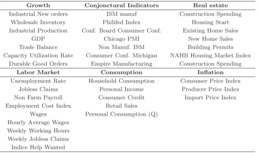
From the Bloomberg database, we also extracted the US economic calendar across the dates already mentioned for the swap rates. This calendar contains every economic an-nouncement linked to the US economy which are supposed to be monitored by financial market participants. Several of these figures are well known by economists, such as the Non Farm Payroll figure, which is the number of jobs created on a one month period. These figures are issued regularly by office statistics such as the Bureau of Labour Statistics. For example, the Non Farm Payroll figure is issued every first Friday of a month and is usually followed by large moves in the bond market. Other figures are no so well known, and one of the purposes of this paper is to cast some light on the effect of these indicators on the term structure of the US swap rates.
Growth Conjonctural Indicators Real estate
Industrial New orders ISM manuf Construction Spending
Wholesale Inventory Philifed Index Housing Start
Industrial Production Conf. Board Consumer Conf. Existing Home Sales
GDP Chicago PMI New Home Sales
Trade Balance Non Manuf. ISM Building Permits
Capacity Utilization Rate Consumer Conf. Michigan NAHB Housing Market Index
Durable Good Orders Empire Manufacturing Construction Spending
Labor Market Consumption Inflation
Unemployment Rate Household Consumption Consumer Price Index
Jobless Claims Personal Income Producer Price Index
Non Farm Payroll Consumer Credit Import Price Index
Employment Cost Index Retail Sales
Wages Personal Consumption (Q)
Hourly Average Wages Weekly Working Hours Weekly Jobless Claims Indice Help Wanted
Table 1: List of the macroeconomic announcements studied in this paper. These announcements are monthly ones, except for: Weekly Jobless Claims (weekly figure), Personal Consumption (quarterly figure), Capacity Utilization Rate (quarterly figure) and GDP (quarterly figure).
We discarded several series from the Bloomberg database. Table 2.1 presents the selected figures used during the estimation process. We eliminated these series for different reasons. First, some of the figures got their names changed over the studied period. In this case, we simply changed the old names into the newer ones so as to avoid having a single figure known under different names. This was the case for the Michigan Consumer Confidence that was reported under several names in the Bloomberg Calendar. Second, some of these figures were ill reported and included a lot of missing values. Finally, some of these figures ceased to be released during the studied period, such as the M3 aggregate and we chose not to include them, to make this study of interest both for academics and practitioners.
Most of the announcements studied are monthly (see Table 2.1). The series were treated by the Bloomberg calendar the way bond market participants do. For example, the surprise in the Consumer Price Index (CPI hereafter) is a surprise in the month-over-month figure. A month-over-month (m-o-m hereafter) figure is simply the percentage of growth of the index over the month. With an index denoted Itfor the month t, the m-o-m figure will be
equal to It
It−1 − 1, with a time unit equal to one month. The same kind of transformation
applies for most of the figures but the sentiment survey such as Purchasing Manager Index (PMI) or Michigan Consumer Confidence. These survey figures are often presented using the value of their index. This is a rather technical knowledge many books are devoted to. Anyone interested in these ways of processing data can get in depth analysis in such books (see e.g. Baumohl (2005)).
In our methodology, we used the first estimates of the macroeconomic news. Most of the macroeconomic figures released in the US are initially preliminary estimates. On the next announcement for the same figure, a revised estimate of the preceding figure is released. Most of the macroeconomic datasets used in empirical papers are made of the revised esti-mates of every macroeconomic figures. Recently, Orphanides (2001), Bernanke and Boivin (2001) and Kishor and Koenig (2005), among others, took this data revision problem into account, highlighting the importance of this phenomenon on macroeconomic empirical models. For our purposes, the use of the first estimate is of tremendous importance: the first announcement is the one bond market participants had to face with and eventually reacted to.
What is more, the Bloomberg calendar also contains the Bloomberg forecasts regarding each of these figures. Bloomberg forecasts are formed using the 50% empirical quantile of the distribution of a survey made of the forecasts of several bank economists, regarding a precise figure. The use of the median as a measure of the expectations makes the forecast robust to the influence of badly intentionned economists that would want to shift the forecast in order to make the most of it. What is more, this forecast is extensively used by market participants. For each figure that is predicted by Bloomberg’s collection of economists’ forecasts, the median is regularly updated until every economist answers the survey, which can take up to two weeks. We retained the last median computed by the Bloomberg services, so as to match both the practioners and academic ways of doing things. Some of the eliminated series were discarded because there was no available forecast.
2.2
Assessing the shape of the market reaction function
In this section, we skip to the presentation of the time series models used along the paper. The first model is the classical linear model. Let St,i denote the surprise at time t in the
figures indexed by i as follows:
St,i=
Rt,i− Ft,i
σSi
, (2)
where Ft,i is the market consensus about the upcoming figures i for t, the date of release;
Rt,i is the real announcement (the first estimate) at time t of the same figure i. To make
the surprises comparable, surprises are scaled using their historical standard deviation. This way of proceeding is very common, see e.g. Edison (1996), Fleming and Remolona (1997, 2001) and Balduzzi et al. (2001).We used the Bloomberg forecasts as a measure of
the market consensus for a given figure at a given date. Thus, Fi
t will be proxyed by the
last forecast in the Bloomberg database for each announcement.
Building a time series model to relate the macroeconomic surprises to the changes in the interest rates of maturity τ requires some preliminary considerations, and especially for the dataset building. Even though there seems to be some regularity in the time of arrival of these surprises, they are irregularly spaced in time, preventing the building of a single global model to relate any surprises to the daily changes in rates. For example, the Non Farm Payroll are scheduled to be released on the first Friday of each month: even though this seems to be a regular release pace, it still leads to data that are irregularly spaced in time, in so far as the number of days from the first Friday of a month to the next one is not always the same. What is more, estimating a global model as asserted before would involve the use of 40 exogenous variables which may threaten the robustness of the results. Moreover, the sampling frequency of the exogenous variables can differ: our work involves both quarterly, monthly and weekly news. Finally, the endogenous variable (namely rt(τ ))
depends on the maturity τ of the swap rates. For several maturities, the model to built should be a generalized linear model (a model that encompasses several dependent vari-ables in the meantime), which thus requires to be estimated using the (Quasi) Generalized Least Squares. To solve these difficulties, we built one model for each each surprise and each maturity, in a similar fashion to the Seemingly Unrelated Regression Models. This has an obvious consequence over the chosen notations: the subscripts must display the dependency on time, maturity and macroeconomic surprise.
Now, let us denote ∆rt,i(τ ) the daily change in swap rate of maturity τ on the date t of the
release of the figure indexes by i = {1, ..., I}, where I is the total number of surprises. The couple (t, i) is somewhat a calendar coordinate in the global dataset. The linear model (model 1 hereafter) assumes for given (fixed) i = {1, ..., I} and τ = {τ1, ...τm} that:
∆rt,i(τ ) = βi,τ + αi,τSt,i+ ǫt,i,τ, (3)
where αi,τ and βi,τ are real-valued parameters. (ǫt,i,τ)t is a Gaussian white noise with
standard deviation σi,τ, conditionally upon St,i. In the remaining of the paper, we denote
these conditions as conditions 2.2. This very simple model is usually augmented with the other surprises announced on the same day (t, i):
∆rt,i(τ ) = βi,τ + αi,τSt,i+ J
X
j=1
γj,τSt,ij + ǫt,i,τ, (4)
where St,ij are the scaled surprises j announced on the same day as surprise i. Again, we
assume that γj,τ,∀j is on the real line. These additional surprises are essential to ensure
that the estimated αi,τ truly isolate the effect of the announcement that is analyzed.
In this section, we build a collection of nested time series models to capture the term structure reaction to macroeconomic news. The linear model defined by equation (3) is the first model. For the ease of the presentation, we will get rid of the part of the equation (4) that is dedicated to the announcements released on the same date as the announcement studied (that is PJj=1γj,τSjt,i), maintaining it during the estimation. What is more, for
the sake of simplicity, we do not denote anymore the maturity of each change in the swap rate, skipping from ∆rt,i(τ ) to ∆rt,i (the same treatment also applies to the parameters
of the model): we present the models for a given and fixed τ .
The immediate consequence of the model 1-like specification is:
E[∆rt,i|St,i] = βi+ αiSt,i. (5)
This expectation has an important implication: whatever past information and the state of the economy, the conditional expectation of the rates’ jump is always the same, for a given surprise, i.e. αiSt,i. This is not in line with what can be observed both by
practi-tioners and academics. We propose two nested non-linear models to account for these facts.
First, with model 1, the market reaction to a given surprise is bound to be the same for each state of the economy. The rates’response to macroeconomic announcements may de-pend on several factors such as the timeliness of the release - that is the order of release for a one month period -, the degree of surprise, the conditions of market uncertainty or the sign of the surprise. On these points, see Fleming and Remolona (1997) and Hans (2001). Other articles pointed toward the fact that the interest rates’response to macroeco-nomic announcements may also depend on a threshold variable, such as ecomacroeco-nomic leading indicators or employment figures. For example, Prag (1994) shows that the impact of unemployment surprises on the bond prices may depend on the current level of unem-ployment. Veredas (2005) shows that the market response to surprises in macroeconomic releases strongly depends upon the momentum of the cycle: in this framework, bad news have more impact on bond prices during expansion periods than recession ones. Here, we argue that the market response depends on several threshold variables, including in-dicators for monetary policy stance and economic agent sentiment regarding future activity.
Thus, we propose to use a threshold time series model. Given the small number of obser-vations we have at hand2
, we will consider a two states economy, say recession/expansion states. Let us define (πt,i)t∈Z, an observable process that is used as a state variable to
capture the conditional reaction to the surprises in the macroeconomic figure i. With this state variable, we measure the state of the economy as follow: this process has to cross a threshold value ¯πifor for the economy to go through a change in state, say from expansion
to recession. For each i ∈ {1, ..., I}, model 2 is then the following:
∆rt,i= βi+ α1,i1πt,i>¯πiSt,i+ α2,i1πt,i≤¯πiSt,i+ ǫt,i, (6)
where 1πt,i>¯πi takes value 1 if πt,i>π¯iand 0 if not. 1πt,i≤¯πi is defined as 1 − 1πt,i>¯πi. α1,i
and α2,iare again on the real line. The assumption 2.2 applies again. This model belongs
to the class of the SETAR models (Self-Exciting Autoregressive models) introduced by Lim and Tong (1980) and developed in Tong (1990).
The estimation of threshold models has been discussed in Chan (1990), Hansen (1997, 2000) and Tong (1990) [chapter 5], and asymptotic estimation results have been derived in it. With these models, the log-likelihood function is not continuous in the threshold pa-rameter. Thus, the threshold cannot be estimated using standard Gradient methods. The estimation can be performed by grid search. This is a standard method in econometrics, as detailed in Greene (2000), in the chapter dedicated to numerical optimization.
2
For monthly figures, we only have one announcement a month, which makes 120 observations with no missing value in the dataset. For the quarterly figures, this makes only 30 observations.
The model proposed in equation (6) leads to the following conditional expectations: E[∆rt,i|πt,i >π¯i, St,i] = βi+ α1,iSt,i (7)
E[∆rt,i|πt,i ≤ ¯πi, St,i] = βi+ α2,iSt,i. (8)
Thus, the market reaction clearly differs, depending upon the state variable. Once again, each macroeconomic figure can be linked to a proper threshold variable (πt,i)t∈Z, along
with a proper threshold value ¯πi. Now, we need to select variables to proxy this state
variable. Clearly, there is no unique answer: sentiment survey (such as PMI index or Con-ference Board index) could be a good proxy for this variable. These sentiment survey can be considered as coincident or leading indicators of the stance of the economy and thus reflects the market sentiment better than real aggregates such as industrial indicators or GDP. Monetary policy is also known to play an important part in the psychology of the bond market. This is why we also introduced the Fed’s target rate, as a measure of the monetary policy stance.
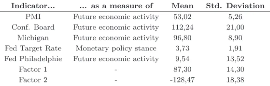
The table 2 presents the different threshold variables that we retained for the estimation of the threshold model. Note that to these variables, we add the first and second factors of a principal component analysis performed over all these variables, so as to get a global economic confidence index. This is a classical method used to build this kind of global economic stance index (see e.g. Stock and Watson (1998)). So as to avoid any data vintage problem, as presented e.g. in Kishor and Koenig (2005), we used the first estimates of ev-ery of these series: they were the ones at hand for market participants, at the time of their reactions to the announcements. In the section dedicated to the estimation results, we present the results of the choice of the threshold variable. For each surprise, we retain the threshold value that yielded the highest log-likelihood value or the lowest root mean square error. These results show the benefit from estimating each model for each macroeconomic figure and each maturities: the selected threshold variable can clearly differ depending both on the rates’ maturity and the figure that is studied.
Indicator... ... as a measure of Mean Std. Deviation
PMI Future economic activity 53,02 5,26
Conf. Board Future economic activity 112,24 21,00
Michigan Future economic activity 96,80 8,90
Fed Target Rate Monetary policy stance 3,73 1,91
Fed Philadelphie Future economic activity 9,54 13,52
Factor 1 - 87,30 14,30
Factor 2 - -128,47 18,38
Table 2: Threshold variables used in the estimation process
In the table presenting the results of our estimations, we refer to these threshold variables using the following notations: PMI is for PMI index, CONF is for Conference Board Con-sumer Confidence, MICH is for ConCon-sumer Confidence Michigan, FED is for the Fed Target Rate, PHI is for the Philifed Index and FACT1 and FACT2 refer to the first two factors of a principal component analysis performed over all these series.
Finally, we propose to test for path dependency in the dynamics of the rates. By this, we simply mean to specify a model that would link the rates’ reaction during two successive announcements of the same figure. Note that most of the time, a month elapsed between
two successive announcements. We propose to test whether a part of ∆rtk,i is explained
by the rates’ reaction at time (tk−1, i), that is the bonds over- or under-reaction during
the former announcement for exactly the same figure i. When model 2 provides consistent estimates of the reaction reaction of the market to announcements, the residuals of this model can be used as a proxy to measure the rates’ over or under reaction to a given announcement. Thus, a natural measure of the market absolute overreaction at time (tk−1, i) is ǫtk−1,i. By adding this term to the model proposed in equation (6), we obtain
model 3:
∆rtk,i= βi+ α1,i1πtk,i>¯πiStk,i+ α2,i1πtk,i≤ ¯πiStk,i+ θǫtk−1,i+ ǫtk,i, (9)
where θi ∈ R such that E[∆rtk,i] < ∞. Conditions 2.2 still apply. By the law of iterated
expectations, E[ǫtk,i] = E[E[ǫtk,i|πtk,i, Stk,i, ǫtk−1,i]] = 0. Thus, we can rewrite equation
(9) with a mean reverting error process:
∆rtk,i= βi+ α1,i1πtk,i>¯πiStk,i+ α2,i1πtk,i≤ ¯πiStk,i− θi(E[ǫtk−1,i] − ǫtk−1,i) + ǫtk,i. (10)
The interpretation of θi in equation (10) arises naturally. Let us distinguish three cases.
If θi = 0, this obviously means that there is no linear link between the past overreaction
and the current one. Second, if θi >0, the bond market tends to be self exciting: when an
over/undershoot occurs when releasing a figure, then there is a higher probability that the market will over/undershoot again on the next release of the same figure. On the contrary, if θi<0, the market responses to announcements are mean reverting (toward a mean equal
to 0). In the latter case, an over/undershoot is likely to be followed by a smoother reaction on the date of the next release of the same figure. Note that from a statistical point of view, if θiis significatively different from 0, the estimation of model 1 is likely to be biased.
The conditional expectation of ∆rtk,i is path dependent: the rates’ response will depend
on their former reaction to the announcement of the same figures. Thus we have:
E[∆rtk,i|πtk,i>π¯i, Stk,i, ǫtk−1,i] = βi+ α1,iStk,i+ θiǫtk−1,i (11)
E[∆rtk,i|πtk,i≤ ¯πi, Stk,i, ǫtk−1,i] = βi+ α2,iSt,i+ θiǫtk−1,i. (12)
From this point, we now obtain a collection of nested models that will help us document further the admissible shapes of the bond market reaction function to macroeconomic an-nouncements. This rather simple approach thus entitles us to build LR tests, as described in Davidson and MacKinnon (1993). Models 1, 2 and 3 are nested, and likelihood ratio tests can be easily performed so as to chose which is the more interesting model, regarding the data at hand. These elements will be studied within the next section, along with the analysis of the results obtained with the models defined by equations (3), (6) and (9). In the remaining of the paper we refer to the model defined by equation (3) as model 1, to the one defined by equation (6) as model 2 and to the model defined by equation (9) as model 3. These notations are summarized in the following table :
Model Equation # Rates dynamic Model 1 Equation (3) ∆rt,i= βi+ αiSt,i+ ǫt,i
Model 2 Equation (6) ∆rt,i= βi+ α1,i1πt,i>¯πiSt,i+ α2,i1πt,i≤¯πiSt,i+ ǫt,i
3
Empirical results
In this Section, we systematically analyse the results of the estimations of the models pre-sented in the previous section. First, we analyse the results obtained from the likelihood ratio tests performed over the different nested models, using the dataset presented earlier. From these estimation results, we propose a list of the most market mover figures for each maturity and we show that by using model 2 the list of market mover figures significatively increases. We also notices that model 2 leads to intercepts that are statistically equal to 0, unlike model 1. Third, we propose to identify the shapes of the term structure response with those of the first four factors of a principal component analysis performed over the daily changes in the swap rates. By doing so, we show that there are several kinds of possible shapes for the hump-shaped term structure response to macroeconomic news (see e.g. Fleming and Remolona (2001)). Fourth, we propose a detailed analysis of the term structure response to several announcements, underlying the fact that the inclusion of a threshold variable reveals that model 1 often underestimates the true reaction function. We guess that this can either be due to the economic cycle dependence of the term struc-ture effect or the existence of outliers within the dataset.
3.1
Bulk effects of the introduction of the threshold variable
The introduction of those threshold variables produced remarkable effects on our estima-tions, yielding results that we believe are new. We present in tables 6, 7 and 8 the results of the estimation obtained from the models presented in the previous section. We only present the estimates of the model with the higher log-likelihood function, along with the following LR test. For example, let model 1 be the constrained model, with log likelihood denoted lnLcand model 2 be the unconstrained model, with a log-likelihood denoted lnLu.
The null hypothesis H0assumes that the constraint imposed in model 1 statistically holds.
Thus, under H0, model 1 is considered as a better model than the unconstrained model.
Tables 6, 7 and 8 report the selected threshold variables along with the threshold value, that are estimated for each maturity and macroeconomic figures. We also report the LR test results, testing constrained against the unconstrained models. The test statistics is:
LR= 2(lnLc− lnLu), (13)
with the previous notations. Under the null hypothesis that the constraint statistically holds, this statistic has a Chi-square distribution, with a degree of freedom equal to the number of constraints imposed in the constraint model. In our case, we have only one con-straint, and the statistics is distributed as a χ2
1, under the null. We proceed in a similar
fashion to test model 3 vs. model 2.
The main result obtained with our methodology is that model 2 is globally the preferred model, regardless of the surprise and the maturity. When testing model 2 vs. model 1, the null is rejected at either a 5% or 10% risk level most of the time for every maturity. The few cases when it is not rejected are reported in table 3. This is an essential result for our work: model 2 provides a better explanation of the rates’ behavior than model 1. Even though model 1 is the one that is generally proposed in the litterature, model 2 better encompases an important feature of the rates’ dynamic: the economic cycle depen-dence. Note that we do not report the LR test of model 3 against model 2, because the
model 3 was almost always rejected at either a 5% or 10% level when compared to model 2.
Economic Announcement Swap rates maturities
Household Consumption 1,6,7,9 and 10 year
Employment Cost Index 15,20 and 30 year
Empire Manufacturing Index 4,5,6,7,8,9,10,15,20 and 30 year
Personal Consumption 2,3,4,5 and 6 year
Table 3: Announcements and maturities for which the null of the LR test is accepted, when testing model 2 vs. model 1.
The introduction of the state variables allowed us to point out more than the usual number of ” market movers” figures: we consider that a market mover figure is an announcement for which the estimated impact in models 1 and 3 is significative up to a 5% percent test. Here, almost every announcement that we tested was found to have a significative influ-ence on the yield curve. Fleming and Remolona (2001) assumed that the use of daily data instead of intra day ones were to bring about an underestimation of the market reaction function. Here, we find that considering the market responses conditionally upon a thresh-old variable that has been properly selected puts an end to this underestimation. Almost every announcement produces an effect on the yield curve. In appendices, we propose two comparative tables to assess this point. In table 9, we present the ranked market mover announcements found when estimating model 1. In tables 10 and 11, we report the ranked market mover announcements obtained when estimating model 2, along with the selected threshold variable and the threshold value. The main point about this table is that the number of market mover figures significantly increases when using model 2: the introduc-tion of the threshold variable leads to the finding of a greater number of market mover figures. The exclusion of this threshold variable seems to bring about an underestimation of the term structure reaction to several announcements. In subsection 3.4, we detail some of the reasons explaining this new stylized fact.
One other remarkable fact about our methodology is the following: when estimating model 1, most of the intercepts are significative up to a 5% risk level, unlike when estimating model 2. Table 4 reports figures and maturities for which this intercept remains significa-tive in model 2. Where the bond market to be efficient, there should be no significasignifica-tive intercept in the estimation of the proposed models. One may think of this constant term as an α in the Capital Asset Pricing Model framework3
, as presented in Gourieroux and Jasiak (2001) and Campbell et al. (1997). Tables 12 and 13 propose the results of the intercept estimation for models 1 and 3. Thus, when compared to model 2, model 1 is misspecified and leads to misleading ideas such as the idea that the bond market is not efficient4
.
3
The CAPM were initially developed by Sharpe (1964), Lintner (1965) and Mossin (1966).
4
In a linear model with centered exogenous variables, the intercept can be interpreted as an average of the endogenous variable. In our case, this means that we are looking for regular effects over a given announcement. This effect is not the result of either a positive or a negative surprise, but simply the result of the fact that on this trading day, the announcement produces by itself a regular reaction in the bond market. Note that swap rates are used for many financial applications, such as deriving zero-coupon yield curve, pricing swaps or pricing interest rates derivatives such as swaptions. This kind of regular moves in the whole bond market can have significant implications for the whole bond market.
Economic Announcement Swap rates maturities Household Consumption 3,4,6,7,8,9,10,15,30
Personal Income 2,3,4,6,7,8,9,10,15,30
ISM Manuf. 4,6,7,8,9,10,15,20,30
Existing Home Sales 8,9,15,20,30
Weekly Jobless Claims 1
Building Permits 1
Empire Manufacturing 1
Personal Consumption 1
Indice Help Wanted 1
NAHB Housing Index 1
Construction Spending 1,7,8,9,10,15,20,30
Table 4: Announcements for which the intercept is significative both for model (1) and model (3)
3.2
Term structure identification
We propose to move a step further toward the analysis of our results. When reading tables 6, 7 and 8, one can clearly see that most of the shapes of the term structure responses to macroeconomic news are hump-shaped, as already noted by Fleming and Remolona (2001). But even though most of them present this kind of shape, while analysing the results, we found different forms of these term structure responses. What is more, these shapes sur-prisingly match those of the correlation between swap rates across maturities and the first four factors of a principal component analysis (PCA hereafter) performed over the daily changes in the swap rates. Since Litterman and Scheinkman (1991), using PCA to assess the shape of the factors that are actually moving the yield curve is very classic. The method is still used for the analysis of bond market factors (see e.g. Lardic and Priaulet (2003)). On this preliminary remark, we propose a methodology to build a classification of the term structure responses of the swap rates to macroeconomic announcement using these four factors.
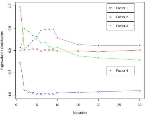
Using the dataset presented in Section 2, we performed a principal component analysis over the daily changes in the swap rates, with maturities ranging from 1- to 30-year. Figure 1 presents the correlations between the first four factors of the PCA and the one-day changes in the swap rate across maturities. Let us denote Ft,k the value of the kthfactor on date t
and ∆rt(τ ) the change in the swap rate of maturity τ on the same date. For the time being,
these notations are independent of the surprises. Then, let us denote ρk,τ the correlation:
ρk,τ = cor (Fk,∆rt(τ )) (14)
where cor(.) is the correlation coefficient. We decided to consider5
factors 1 to 4, using the classical elbow method to select the number of eigenvalues and eigenvectors to retain for this PCA. By studying the ρk,τ, we are able to discuss the impact of the factor k on the
yield curve. Figure 1 presents the correlations between each factor and the jumps in swap rates for a given maturity. Clearly, these factors do not seem to have the same impact on the yield curve. Factor 1 is considered as a level factor and is often related to the mone-tary policy stance (see e.g. Bomfim (2003), Wu (2001) and Ang et al. (2005)). Factor 2 is extremely well positively correlated (close to one) with the changes in one-year swap rates and thus governs the slope of the beginning of the yield curve. Factor 3 is highly correlated
5
Most of the studies achieved so far concluded with the fact that three factors were actually driving the pure discount bond yield curve. To our mind, one key explanation for this divergence with the classical literature is due the fact we use a very recent dataset.
to the swap rates of maturities 2 to 7 years and thus drives the concavity of the curve. Finally, the fourth factor is well correlated to maturities a bit longer than factor 3, that is maturities from 6 till 9 years, and is thus again a concavity factor. These results can also be found in other articles such as Steeley (1990), Litterman and Scheinkman (1991), Knez et al. (1994) and more recently Molgedey and Galic (2000) and Blaskowitz et al. (2005).
In this respect, our analysis identifies four types of factors: a first type that seems to be hump-shaped and should be theoretically driven by the conduct of monetary policy; a second type affecting mainly the short rate positively; a third type affecting negatively maturities for 2 to 7 years and a fourth one affecting negatively maturities from 6 to 9 years.
0 5 10 15 20 25 30 −1.0 −0.5 0.0 0.5 1.0 Maturities Eigenvalues / Correlations Factor 1 Factor 2 Factor 3 Factor 4
Figure 1: Correlations between factors 1 to 4 and the jumps in rates for maturities till 30 years
Noting that the shapes of the impact of the surprises on the yield curve are graphically close to the shapes of the correlations ρk,τ across maturities, we propose an identification
process to be able to match the effect of the announcements to the factors of the PCA. We propose the following method. Let αi,τ be the estimate of the impact of the announcement
ion the change in swap rate for a maturity τ . Thus, we have:
∆rt,i(τh) = βi,τ + αi,τSt,i+ ǫt,i,τ, (15)
under the assumptions 2.2. Now, for a given announcement i, we propose to compare ρk,τ
and αi,τ across maturities , for each factor k. Note that the αi,τ can either be estimated
with model 1, 2 or 3: we present the methodology using model 1 as an example for the sake of notational simplicity. From now on, we propose to state that an announcement
i produces a factor k-like effect on the yield curve when the distance between ρk,τ and
αi,τ is the lowest across maturities τ and among the different possible factors. For this
purpose, we propose to estimate the following linear model for each factor k and for a given announcement i:
αi,τ = γ0+ γ1ρk,τ+ νk,τ,∀τ, (16)
and retain the estimated variance of νk,τ as a distance measure between αi,τ and ρk,τ.
In equation (16), γ0 and γ1 are real-valued parameters estimated by OLS. νk a Gaussian
white noise, with variance σ2
k. Now, for example, if σ1 2 is inferior to σ2 2, σ 2 3 and σ 2 4 for a
given surprise i, then we say that this surprise produce a factor 1-like effect on the yield curve.
In table 14, we report the results of the latter method, using the estimation results obtained with model 2. Table 5 provides empirical frequencies regarding the number of announce-ments per yield curve factor. Most of the announceannounce-ments seem to match the factor 1 of the yield curve, but we found many other announcements matching the remaining factors. We believe that the results presented here are new, along with the idea that there are several types of shapes for the term structure announcements.
Factor 1 Factor 2 Factor 3 Factor 4
Number 29 11 6 5
Total number 54 54 54 54
Empirical Frequency 0,54 0,20 0,11 0,09
Table 5: Number of announcements matching one of the factors of the yield curve found during the estimation process.
Now, an in depth analysis of the estimation tables yield two different findings: first, each announcement can have a different term effect on the term structure of the interest rates. While reading the estimation tables, what can be clearly noted is that most of the figures lead to a hump-shaped reaction function (a factor 1-like effect). Once the PCA is per-formed, this result should not surprise anyone: the first factor, that is the hump shaped one, is supposed to explain more than eighty percent of the total variance of the overnight change in swap rates sample at hand. Nevertheless, this kind of shape is not the only one that the results pointed out: we found three other shapes that clearly match that of the three remaining factors extracted using PCA. One supporting fact of our findings is that the empirical frequencies associated to this classification are quickly decaying, just like when analysing the eigenvalues obtained when performing a PCA over the rates. We believe that this fact is new. Second, we found that when modifying the threshold variable and the threshold value, a similar announcement can have different effects on the yield curve, depending upon the state of the US economy for example. A careful reading of table 14 should provide important results both to academics and practioners. We will document this point in the next subsection with well chosen examples.
3.3
Selected announcements and the underestimation problem
In this subsection, we detail with a greater attention some of the results we thought of interest, regarding the economic cycle dependence and the effects of the outliers on the estimations.
3.3.1 The economic cycle effect
We found several types of statistical effects linked to the introduction of the threshold variables that we thought of equal importance. As we initially used these variables for, we came to be able to separate the bond market reaction function to announcements during expansion and recession cycles. Three types of results arose: first, some announcements were found to have a sharper effect on the yield curve during either the recession or the expansion period, matching in both these cases the same factor pattern. Second, some announcements seemed to have an effect during only one of those periods, and no effect during the other one. Third, a few announcements were found to have a different type of effect on the yield curve, depending upon the threshold variable. In such a case, the global stance of the economy not only influences the strength of the market response to some surprises: it also brings about a change in the type of term structure of the rates’ response to surprises. We propose hereafter some examples of these statistical effects that we found within our estimations.
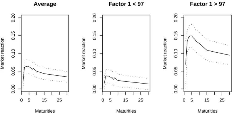
First, some of the figures were found to have a sharper effect on the changes in US swap rates when the threshold variable lies below or above the estimated threshold. What is more, the average effect of the announcement usually under- or over-estimates the actual term structure of the swap rates’ response. The announcement of Non-farm Payroll is a good example of such a pattern. As presented in figure 2, the average effect (i.e. estimated with model 1) of the announcement lies typically below (above) the one obtained when considering the sample for which the threshold variable lies above (below) the estimated threshold. This has important implications for the building of interest rates models, both for professionals of finance and for monetary policy makers: the Non Farm Payroll (NFPR hereafter) figure is not that closely monitored by financial markets during slowdown pe-riods, but is of tremendous importance during expansion ones. What is more, the term structure reaction matches factor 1 for both cases, suggesting that this variable is inter-preted by financial markets as monetary policy driving figure.
Second, for some figures, only one period includes a significative term structure reaction of the US swap rate. The average effect (estimated with model 1) is not significative and only one of the two states associated to model 3 yields significative estimates. The Capacity Utilization Rate is an example of this phenomenon: when the Fed’s target rate is above 3.5%, the term structure effect is globally equal to zero. On the contrary, when the target rate is below 3.5%, one gets an important hump-shaped reaction function. This effect is presented in figure 3. Again, this has important implications for the understanding of the reaction of interest rates to macroeconomic announcements. What is more, this type of effect could explain the fact that high-frequency dataset led to the finding of more market mover figures than the daily ones.
0 5 15 25 0.00 0.05 0.10 0.15 0.20 Maturities Market reaction Average 0 5 15 25 0.00 0.05 0.10 0.15 0.20 Maturities Market reaction Factor 1 < 97 0 5 15 25 0.00 0.05 0.10 0.15 0.20 Maturities Market reaction Factor 1 > 97
Figure 2: Swap rates reaction function to a positive surprise for Non Farm Payroll (plain line) and 95% confidence intervals (dotted lines).
Finally, the most striking effect is for figures that lead to different types of shapes of the term structure responses, depending upon the level of the threshold variable. Until now, we simply underlined figures for which we found the same term structure effect across the different values of the threshold variable. But for some figures, the term structure effect seems to depend on the state of the economy. This means that the interpretation of the signal driven by these variables is state-dependent. One example of such pattern is the Construction Spending figure. Figure 4 presents the different patterns of the term structure reaction of the swap rates to positive surprises, depending on whether the Philifed index is above or below 2. Philifed Index is a sentiment survey. Depending upon the threshold variable, we obtain two different patterns: a positive reaction function that is close to the factor 3 shape when the Philifed is above 2 and a negative hump-shaped one that is close to the factor 1 pattern when the Philifed is below 2. This means that the market perception of construction spendings strongly depends on the state of the economy.
0 5 15 25 0.0 0.1 0.2 0.3 0.4 0.5 Maturities Market reaction Average 0 5 15 25 0.0 0.1 0.2 0.3 0.4 0.5 Maturities Market reaction Target rate > 3.5 0 5 15 25 0.0 0.1 0.2 0.3 0.4 0.5 Maturities Market reaction Target rate < 3.5
Figure 3: Swap rates reaction function to a positive surprise for Capacity Utilization Rate (plain line) and 95% confidence intervals (dotted lines).
3.3.2 The outliers effect
Some recent papers using high frequency datasets (e.g. Fleming and Remolona (2001)) found a greater number of market mover figures than usually found in daily datasets. Our estimations results produced one possible explanation for this phenomenon. The existence of outliers within the changes in the swap rates across maturities leads to biased estima-tions of the term structure reaction. This is in line with what has been said in the previous section: the sample splitting produced by the introduction of a threshold variable led to the assessment of an over- or under-estimation of the bond market reaction function. This phenomenon is often referred to as aliasing, and is well known and diagnosed using jump models (see e.g. Andersen et al. (2003a)). Note that Andersen et al. (2003a) directly encourage empirical papers investigating the types of issue we are faced with6
.
These outliers generally appear when the global economic stance of the US is very high or very low, that is to say close to turning points in the economy. Bond markets seem to have odd reactions when getting near these turning points. In fact, one can assume that during these periods, the expectations of bond market participant are very sensitive to any breaking news in the economy. Turning points in the economy are very important in so far as they match the inversion of the central bank policy. When the Fed comes to the end of a tightening cycle, the turning point will trigger the beginning of an easing cycle of the monetary policy and a progressive reduction of the target rate. In this perspective, the forward rates, and thus the spot rates are very sensitive to these changes in economic perspectives.
The estimation results presented in tables 6, 7 and 8 point toward the fact that getting rid of these outliers brings about a reduction of the estimation bias in the bond markets’ term
6
Here is the quote taken from Andersen et al. (2003a): ”These daily jump proportions are much higher than the jump intensities typically estimated with specific parametric jump diffusion models applied to daily or coarser frequency returns. This suggests that many of the jumps identified by the high-frequency based realized volatility measures employed here may be blurred in the coarser daily or lower frequency returns through an aliasing type phenomenon. [...] The fixed income market is generally the most responsive to macroeconomic news announcements (e.g., Andersen et al. (2003b)). Along these lines, it would be interesting, but beyond the scope of the present paper, to directly associate the significant jumps identified here with specific news arrivals, including regularly-scheduled macroeconomic news releases.”
0 5 10 15 20 25 30 −0.10 −0.05 0.00 0.05 Maturities Market reaction Average 0 5 10 15 20 25 30 −0.10 −0.05 0.00 0.05 Maturities Market reaction Philifed < 2 0 5 10 15 20 25 30 −0.10 −0.05 0.00 0.05 Maturities Market reaction Philifed > 2
Figure 4: Swap rates reaction function to a positive surprise for Construction Spending (plain line) and 95% confidence intervals (dotted lines).
structure reaction function. Here again, we found three types of effects: a first one for which we observed an underestimation of the rates’ reaction function to macroeconomic announcements, when the effect of the announcement were already considered significant for model 1; a second one that is related to announcements for which the response is primarily found not to be significative when the outliers are maintained in the dataset, and significative if not; a third one, for which, in case of extreme economic situation, the market seems to have an significative reaction function.
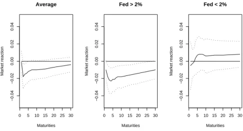
First, when the sample splitting leads to the elimination of a few outliers, the estimated term structure reaction function may be more important for the sample that excludes the outliers. This is for example the case of the Durable Good Orders and of the Philifed Index. When estimating the swap rate reaction function to such announcements with model 1, one would find significative estimates. Nevertheless, the estimates obtained in the threshold model are more significant and present a superior absolute value, when the selected threshold variable is above or below the estimated threshold value. Figure 5 presents the term structure reaction to the announcement of the Durable Good Orders, when the Fed fund target rate is below or above 2%.
0 5 10 15 20 25 30 −0.04 −0.02 0.00 0.02 0.04 Maturities Market reaction Average 0 5 10 15 20 25 30 −0.04 −0.02 0.00 0.02 0.04 Maturities Market reaction Fed > 2% 0 5 10 15 20 25 30 −0.04 −0.02 0.00 0.02 0.04 Maturities Market reaction Fed < 2%
Figure 5: Swap rates reaction function to a positive surprise for Durable Goods Orders (plain line) and 95% confidence intervals (dotted lines).
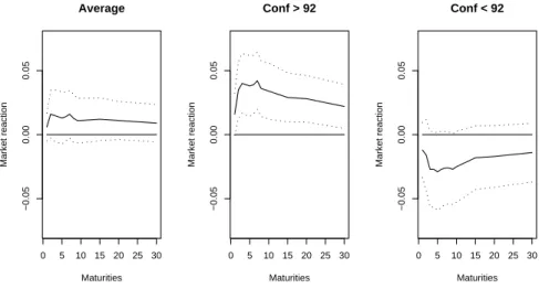
Secondly, the estimation of the impact of some of the studied figures leads to the finding of no remarkable effect on the yield curve when using model 1. The exclusion of the outliers from the dataset then brings about very different estimation results, suggesting that the first estimates were biased because of the presence of these extreme values. Good examples of this fact are the Unemployment Rate and the Weekly Working Hours. Without the sample splitting process, one would conclude with the fact that these announcements do not have any effect on swap rates. When implementing our methodology, we find that the shape and the significativeness of the term structure’s reaction function of the swap rates is clearly very different. In figure 6 we present the term structure of the announcement effect of the Weekly Working Hours on the swap rates curve, documenting what has just been said.
0 5 10 15 20 25 30 −0.05 0.00 0.05 Maturities Market reaction Average 0 5 10 15 20 25 30 −0.05 0.00 0.05 Maturities Market reaction Conf > 92 0 5 10 15 20 25 30 −0.05 0.00 0.05 Maturities Market reaction Conf < 92
Figure 6: Swap rates reaction function to a positive surprise for Weekly Working Hours (plain line) and 95% confidence intervals (dotted lines).
Finally, a last type of effects appeared in the estimation results: some of the studied figures produce no significative effect on the yield curve when estimating model 1, but during very special occasions can have a dramatic impact across maturities. For a few outliers, the response of the swap rates is again important and hump-shaped. The Industrial Orders fig-ure is a good example of such a pattern: the model presented in Section 2 that maximized the log-likelihood was the one using the PMI (Purchasing Manager Index) as a threshold variable. When the PMI index is below 42, which is rarely the case, the term structure of the rates’ reaction is significative for each maturity. On the contrary, when the PMI is above 42, we did not find any observable effect. This is presented in figure 7. One should remain cautious regarding the interpretation of this finding. The few observations for this type of event makes it hard to be very conclusive. Nevertheless, the fact we have again a hump-shaped reaction function tends to support the idea that industrial orders are a closely-watched figure in financial markets when getting closer to the end of the slowdown cycle of the economy.
Conclusion
The aim of this paper was to estimate a collection of nested time series models for data-mining purposes. We found several new results. First, the use of a threshold model for the analysis of the term structure effect of macroeconomic announcements yields a much longer list of market mover figures. Second, we found that the classical hump-shaped term structure reaction function of interest rates to market mover announcements was not the only existing shape. At least three to four shapes may have to be considered, surprisingly matching that of the first four factors of a PCA performed over the daily changes in the shape rates. We develop a distance measure to build a classification of the term structure effect of announcements on the yield curve. Third, we found that the introduction of a state variable often leads to a better understanding of the reaction function to most of the announcements. When the economy is slowing or roaring, the impact of the surprises
0 5 10 15 20 25 30 −0.04 −0.02 0.00 0.02 0.04 Maturities Market reaction Average 0 5 10 15 20 25 30 −0.04 −0.02 0.00 0.02 0.04 Maturities Market reaction PMI > 42 0 5 10 15 20 25 30 0.0 0.2 0.4 0.6 Maturities Market reaction PMI < 42
Figure 7: Swap rates reaction function to a positive surprise for Industrial Orders (plain line) and 95% confidence intervals (dotted lines).
in the announcements is obviously not the same. It can even change the shape of the term structure reaction itself. Fourth, the sample splitting used throughout the paper make it possible to isolate a few outliers and to analyse the rates dynamics on each sample separately. The results point toward the fact that these outliers often bring about an underestimation of the reaction function.
References
Andersen, T. G., Bollerslev, T., and Diebold, F. X. (2003a). Some like it smooth, and some like it rough: Untangling continuous and jump components in measuring, modeling, and forecasting asset return volatility. CFS Working Paper Series 2003/35, Center for Financial Studies.
Andersen, T. G., Bollerslev, T., Diebold, F. X., and Vega, C. (2003b). Real-time price discovery in stock, bond and foreign exchange markets. PIER Working Paper Archive 04-028, Penn Institute for Economic Research, Department of Economics, University of Pennsylvania.
Ang, A., Dong, S., and Piazzesi, M. (2005). No-arbitrage taylor rules. Working Paper, Columbia University.
Balduzzi, P., Elton, E. J., and Green, T. C. (2001). Economic News and the Yield Curve: Evidence from the U.S. Treasury Market. Journal of Financial and Quatitative Analysis, 36(4):523–543.
Baumohl, B. (2005). The Secrets of Economic Indicators. Wharton School Publishing, University of Pennsylvania, USA.
Bernanke, B. S. and Boivin, J. (2001). Monetary Policy in a Data-Rich Environment. NBER Working Papers 8379, National Bureau of Economic Research, Inc.
Blaskowitz, O., Herwartz, H., and de Cadenas Santiago, G. (2005). Modeling the FI-BOR/EURIBOR Swap Term Structure: An Empirical Approach. SFB 649 Discussion
Papers SFB649DP2005-024, Sonderforschungsbereich 649, Humboldt University, Berlin, Germany.
Bomfim, A. N. (2003). Monetary policy and the yield curve. Finance and Economics Discussion Series 2003-15, Board of Governors of the Federal Reserve System (U.S.). Campbell, J., Lo, A., and MacKinlay, C. (1997). The econometrics of financial markets.
Princeton University Press, New Jersey.
Chan, K. S. (1990). Testing for Threshold Autoregression. Ann. Statist., 4:1886–1894. Chen, R.-R. and Scott, L. (1993). Maximum Likelihood Estimation of a Multifactor
Equilibrium Model of the Term Structure of Interest Rates. Journal of Fixed Income, 3:14–31.
Cox, J., Ingersoll, J., and Ross, S. A. (1985). A Theory of the Term Structure of Interest Rates. Econometrica, 53:385–407.
Davidson, R. and MacKinnon, J. G. (1993). Estimation and Inference in Econometrics. Oxford University Press.
Edison, H. J. (1996). The reaction of exchange rates and interest rates to news releases. International Finance Discussion Papers 570, Board of Governors of the Federal Reserve System (U.S.).
Fleming, M. J. and Remolona, E. M. (1997). What moves the bond market? Research Paper 9706, Federal Reserve Bank of New York.
Fleming, M. J. and Remolona, E. M. (2001). The Term Structure of Announcement Effects. Staff Reports 76, Federal Reserve Bank of New York.
Gourieroux, C. and Jasiak, J. (2001). Econometrics of Finance. Princeton University. Greene, W. (2000). Econometric Analysis. Prentice-Hall International.
Grossman, J. (1981). The ’Rationality’ of Money Supply Expectations and the Short-Run Response of Interest Rates to Monetary Surprises. Journal of Money, Credit and Banking, 13:409–424.
Hans, D. (2001). Surprises in U.S. Macroeconomic Releases: Determinants of Their Rel-ative Impact on T-Bond Futures. Center of Finance and Econometrics, University of Konstanz, (Discussion Paper No. 2001/01).
Hansen, B. E. (1997). Inference in tar models. Studies in Nonlinear Dynamics and Econo-metrics, 2:1–14.
Hansen, B. E. (2000). Sample splitting and threshold estimation. Econometrica, 68(3):575– 604.
Hardouvelis, G. (1988). Economic News, Exchange Rates and Interest Rates. Journal of International Money and Finance, 7:23–35.
Kishor, N. and Koenig, E. (2005). VAR Estimation and Forecasting when Data Are Subject to Revision. Working Papers 05-01, Federal Reserve Bank of Dallas.
Knez, P. J., Litterman, R., and Scheinkman, J. A. (1994). Explorations into factors explaining money market returns. Journal of Finance, 49(5):1861–82.
Lardic, S. and Priaulet, P. (2003). Answers about PCA Methodology on the Yield Curve. Journal of Bond and Management Trading, 4:327–349.
Lim, K. and Tong, H. (1980). Threshold Autoregression, Limit Cycles and Cyclical Data. J. Roy. Statist. Soc., 42:245–292.
Lintner, J. (1965). Valuation of Risky Assets and the Selection of Risky Investments in Stock Portfolio and Capital Budgets. Review of Economics and Statistics, 47:13–37. Litterman, R. and Scheinkman, J. (1991). Common Factors affecting Bond Returns.
Jour-nal of Fixed Income, 1:54–61.
Martellini, L., Priaulet, P., and Priaulet, S. (2003). Fixed Income Securities : Valuation, Risk Management and Portfolio Strategies. Wiley.
Molgedey, L. and Galic, E. (2000). Extracting Factors for Interest Rate Scenarios. The European Physical Journal, B20:517–522.
Mossin, J. (1966). Equilibrium in Capital Asset Market. Econometrica, 35:768–783. Orphanides, A. (2001). Monetary Policy Rules Based on Real-Time Data. American
Economic Review, 91(4):964–985.
Piazzesi, M. and Swanson, E. (2004). Futures Prices as Risk-adjusted Forecasts of Mon-etary Policy. NBER Working Papers 10547, National Bureau of Economic Research, Inc.
Prag, J. (1994). The Response of Interest Rates to Unemployment Rate Announcements: Is there a Natural Rate of Unemployment. Journal of Macroeconomics, 16:171–184. Sharpe, W. (1964). Capital Asset Prices: A Theory of Market Equilibrium Under
Condi-tions of Risk. Journal of Finance, 84:425–442.
Steeley, J. (1990). Modelling the Dynamics of the Term Structure of Interest Rates. Economic and Social Review, Symposium on Finance, 21(4):337–361.
Stock, J. H. and Watson, M. W. (1998). Diffusion Indexes. NBER Working Papers 6702, National Bureau of Economic Research, Inc.
Tong, H. (1990). Non-linear Time Series: A Dynamical System Approach. Oxford Univer-sity Press, Oxford, UK.
Urich, T. and Watchel, P. (1981). Market Response to the Weekly Money Supply An-nouncements in the 1970’s. Journal of Finance, 36:1063–1072.
Vasicek, O. (1977). An Equilibrium Characterization of the Term Structure. Journal of Financial Economics, 5:177–188.
Veredas, D. (2005). Macroeconomic Surprises and Short Term Behavior in Bond Futures. Empirical Economics, 30:791–794.
Wu, T. (2001). Monetary policy and the slope factor in empirical term structure estima-tions. Working Papers in Applied Economic Theory 2002-07, Federal Reserve Bank of San Francisco.