HAL Id: inria-00122924
https://hal.inria.fr/inria-00122924
Submitted on 5 Jan 2007
HAL is a multi-disciplinary open access
archive for the deposit and dissemination of
sci-entific research documents, whether they are
pub-lished or not. The documents may come from
teaching and research institutions in France or
abroad, or from public or private research centers.
L’archive ouverte pluridisciplinaire HAL, est
destinée au dépôt et à la diffusion de documents
scientifiques de niveau recherche, publiés ou non,
émanant des établissements d’enseignement et de
recherche français ou étrangers, des laboratoires
publics ou privés.
and Determinacy
Denis Caromel, Ludovic Henrio
To cite this version:
Denis Caromel, Ludovic Henrio. Asynchonous Distributed Components: Concurrency and
Determi-nacy. Theoretical Computer Science 2006 (IFIP TCS’06), 2006, Santiago, Chile. �inria-00122924�
Concurrency and Determinacy
Denis Caromel Ludovic Henrio
CNRS – I3S – Univ. Nice Sophia Antipolis – INRIA Sophia Antipolis Inria Sophia-Antipolis,2004 route des Lucioles – B.P. 93
F-06902 Sophia-Antipolis Cedex {caromel, henrio}@sophia.inria.fr
Abstract. Based on the impς-calculus, ASP (Asynchronous Sequen-tial Processes) defines distributed applications behaving determinis-tically. This article extends ASP by building hierarchical and asyn-chronous distributed components. Components are hierarchical - a com-posite can be built from other components, and distributed - a compos-ite can span over several machines. This article also shows how the asynchronous component model can be used to statically assert compo-nent determinism.
1 Introduction
The advent of components in programming technology raises the question of their formal ground, intrinsic semantics, and above all their compositional se-mantics. It represents a real challenge as practical component models are usually quite complex, featuring distribution over local or wide area networks. But, few formal models for component were proposed so far [4, 20, 3, 14]. Since the first ideas about software components, usually dated in 1968 [1], the design of a reusable piece of software has technically evolved. From the first off-the-shelf modules, a component has become a complex piece of parameterized code with attributes to be set. Its behavior can be adapted with various non functional as-pects (life-cycle, persistence, etc.). Finally, such piece of code is to be deployed in a hosting infrastructure, sometimes it can also be retrieved for replacement with a new version. In recent years, one crucial new aspect of component has been introduced: not only the interfaces being offered are specified, but also the needed interfaces.
A first key aspect of our work is to take into account this feature: the model being proposed allows to specify that a software components provides well de-fined interfaces, and requires well dede-fined services or interfaces. A second and important contribution is to take into account components that are distributed over several machines. A given component can span as a unique entity over sev-eral hosts in the network. This work go further than a distributed-component infrastructure just allowing two components to talk over the network. Finally, the components being proposed are hierarchical (allowing a compositional
spec-ification and verspec-ification of the behavior of large scale systems), communicating with remote method invocations (versus raw messages), and as much as possible decoupled (asynchronous to scale over large area networks).
When building some kind of component calculus, one has the option to start from scratch, or on the contrary to rely as much as possible on syntax and semantics of a programming calculus. This paper clearly takes the latter approach, relying as much as possible on a long history of research on concurrent and distributed calculi. It is in accordance with the practical situation where component infrastructure is usually added on top of a programming language. The main contributions of this paper are:
– a formalization of a component model featuring distribution, asynchrony, and hierarchical composition; with two translations defining the semantics; – usage of components as a convenient abstraction for statically ensuring
de-terminism, which, to our knowledge, is a totally novel approach.
This article is first a direct formalization of the component model imple-mented in ProActive [5, 11]. More generally, our distributed component model is minimally characterized by asynchronous components, hierarchy, no shared memory, and a single threaded lowest level of components; thus, it can be adapted to turn any object model into distributed decoupled components com-municating by structured method calls.
Taking advantage of ASP and its properties [10], summarized in Section 2, this article provides a formal syntax for the description of distributed com-ponents in Section 3. Then, Section 4 shows an example of a deterministic component. Two translational semantics are given in Section 5. Finally, com-ponents provide a suitable abstraction for statically identifying deterministic programs as shown in Section 6.
2 Background
2.1 Some Related Works
ASP is based on the untyped imperative object calculus of Abadi and Cardelli [2], with a local semantics inspired from [15]. Futures [16, 13] are used to represent awaited results of remote calls, determinism is strongly related to process net-works [17], and linear channels [18]. A comparison of ASP with other calculi can be found in [10, 9].
Components over Actors are presented in [4], compared to our work, Actor components neither are hierarchical nor benefit from the notion of futures. Moreover, the communication and evaluation model of Actors cannot guarantee the causal ordering and determinism properties featured by ASP. [3] focuses on the definition of connection and interactions, and on the specification on the behavior. Connectors having their own activity it is impossible to adapt our determinism properties to Wright.
Stefani et al. [6, 20] introduced the kell calculus that is able to model com-ponents and especially sub-comcom-ponents control. We rather demonstrate how to build distributed components that behave deterministically and for which the deterministic behavior is statically decidable. Moreover, the properties shown here rely on properties of communications and semantics of the calculus that are not ensured directly by the kell calculus, and its adaptation would be more com-plicated than the new calculus presented here. However, those two approaches being rather orthogonal, one could expect to benefit of both by adapting a kell calculus-like control of components with an (adaptation of) ASP as the un-derlying calculus. Bruneton, Coupaye and Stefani also proposed a hierarchical component model: Fractal [12], together with its reference implementation Ju-lia [7]. Our work can also be considered as a foundation for distributed Fractal components, focusing on the hierarchical aspect rather than on the component control.
2.2 ASP Calculus: Syntax and Informal Semantics
The ASP calculus [10], is an extension of the impς-calculus [2, 15] with two primitives (Serve and Active) to deal with distributed objects. The ASP cal-culus is implemented as a Java library (ProActive [11]). ASP strongly links the concepts of thread and of object, it is minimally characterized by:
– Sequential activities: each object is manipulated by a single thread, – Communications are asynchronous method calls, and
– Futures as first class objects representing awaited results.
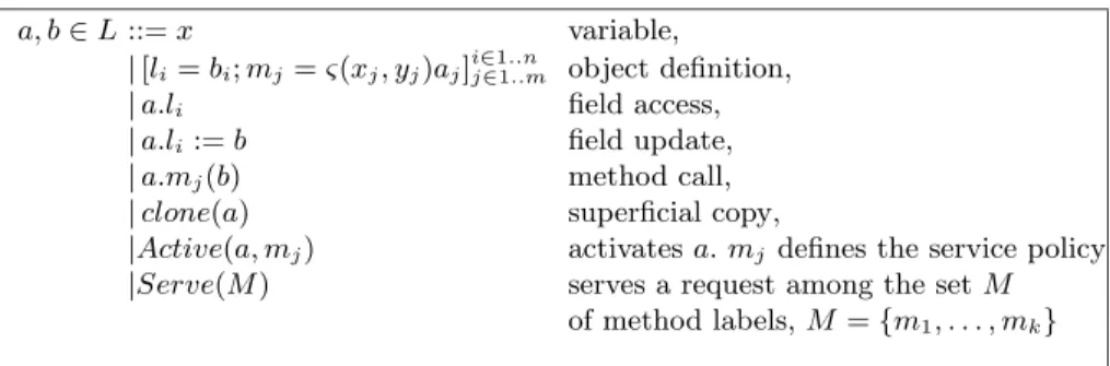
a, b∈ L ::= x variable,
| [li= bi; mj= ς(xj, yj)aj]i∈1..nj∈1..m object definition,
| a.li field access,
| a.li:= b field update,
| a.mj(b) method call,
| clone(a) superficial copy,
|Active(a, mj) activates a. mj defines the service policy
|Serve(M ) serves a request among the set M
of method labels, M = {m1, . . . , mk}
Fig. 1. ASP Syntax (li are fields names, mj are methods names)
ASP is formalized as follows. An activity (denoted by α, β, γ, . . . ) is com-posed of a thread manipulating a set of objects put in a store. The primitive Active(a, m) creates a new activity containing the object a which is said ac-tive, m is a method called upon the activity creation. Every request (method call) sent to an activity is actually sent to this master object. An activity also
contains the pending requests (requests that have been received and should be served later) and the computed results of the served requests (future values). AO(α) represents a reference to the remote active object of activity α. A paral-lel configuration (denoted by P , Q, . . . ) is a paralparal-lel composition of activities: P, Q::= α[aα; σα; ια; Fα; Rα; fα]kβ[. . .]k . . . where aαis the term currently
eval-uated in α, σα is the store (association between locations ιi and objects), ιαis
the location of the active object inside σα, Fα is the list of calculated futures,
Rαis the request queue, and fα is the future corresponding to aα.
Futures are generalized references that can be manipulated as local ones, they can be transmitted to other activities; and future identifiers are unique for the whole configuration. But, upon a strict operation (field or method access, field update, clone) on a future, the local execution is stopped until the value of the future is updated.
Calling a method on an active object atomically adds a new entry in a request queue, associates a future to the response and deep copies the argument of the request in the store of the destination activity. Deep copy allows one to prevent distant references to passive objects, synchronous request delivery ensures causal order between requests. The primitive Serve(M ) can appear at any point in the source code. Its execution stops the activity until a request on one of the methods of the set M is found in the request queue. The oldest such request is then removed from the request queue and executed (served).
Once the response to a request is computed, the corresponding value (future value) becomes available and every activity can get it. The futures associated with the currently served requests are called the current futures. Returning the value associated to a future (also called “updating a future”), consists in replacing reference to a future by a deep copy of the future value. We proved that the value of a future can be returned at any time without any consequence on the execution.
An operational semantics for ASP has been detailed in [10] and is denoted by −→. It is based on a classical local reduction (→S) on ς-calculus terms [2]. This
reduction specifies a single reduction point inside each activity which ensures a local sequentiality. R[a] denotes a reduction context, where the reduction point is inside a; thus aα = R[ι.mj(ι0)] means the next reduction of activity α will
consist in performing a method call on the object referenced (locally) by ι; if moreover σα(ι) = AO(β) then this is a remote method call to activity β.
∗
−→ denotes the reflexive transitive closure of −→.
2.3 ASP Properties: Deterministic Objects Networks
This section presents the properties of the ASP calculus; mainly it recalls the definition of deterministic object networks which identifies a set of ASP terms that behave deterministically. Though DON terms are based on an intuitionist notion: “non-determinism only originate from conflicting requests”; ASP is the first calculus to feature such a property for concurrent imperative objects.
In the following, αP denotes the activity α of configuration P . Without any
restriction, and to allow comparison based on activities identifiers, we suppose that the freshly allocated activity names are chosen deterministically: the first activity created by α will have the same identifier for all executions.
Potential Services Let MαP be an approximation of the set of M that can appear in the Serve(M ) instructions that the activity α may perform in the future. In other words, if an activity may perform a service on a set of method labels, then this set must belong to MαP:
∃Q, P −→ Q ∧ a∗ αQ= R[Serve(M )] ⇒ M ∈ MαP This set can be specified by the programmer or statically inferred.
Interfering Requests Two requests on methods m1 and m2 are said to be
interfering in α in a program P if they both belong to the same potential service, that is to say if they can appear in the same Serve(M ) primitive:
Requests on m1and m2are interfering if {m1, m2} ⊆ M ∈ Mαp Equivalence Modulo Replies ≡F, defined in [9], is an equivalence relation
considering references to futures already calculated as equivalent to local refer-ence to the part of store which is the (deep copy of the) future value.
More precisely, ≡F is an equivalence relation on parallel configurations
mod-ulo the renaming of locations and futures and permutations of requests that cannot interfere. Moreover, a reference to a future already calculated (but not locally updated) is equivalent to a local reference to the (part of the store which is the) deep copy of the future value.
Deterministic Object Networks If two interfering requests cannot be sent to the same destination (β below) at the same moment then the program be-haves deterministically. Of course, two such request would originate from two different activities (αQ). “there is at most one” is denoted by ∃1.
Definition 1 (DON) A configuration P , is a Deterministic Object Network (DON (P )) if it cannot be reduced to a configuration where two interfering re-quests can be sent concurrently to the same destination activity:
P −→ Q ⇒ ∀β ∈ Q, ∀M ∈ M∗ βQ, ∃1α
Q∈ Q, ∃m ∈ M, ∃ι, ι0, aαQ= R[ι.m(ι
0)] ∧ σ
αQ(ι) = AO(β)
Theorem 1 (DON determinism). DON(P ) ∧ P −→ Q∗ 1 ∧ P −→ Q∗ 2 ⇒ ∃R1, R2, Q1−→ R∗ 1 ∧ Q2−→ R∗ 2 ∧ R1≡F R2
DON(P ) ensures that, for all orders of request sending, we always serve the requests in the same order. Thus, provided no two requests can be sent at the same moment on the same potential service of a given destination, the consid-ered program behaves deterministically. Section 6 will show how components can ensure this statically.
3 Distributed Components
This section demonstrates how to build hierarchical and distributed compo-nents upon ASP. The asynchronous compocompo-nents presented below interact with method calls in an object-oriented way. The component specification presented in this section can be viewed as an abstraction of a classical ADL (e.g. the Fractal ADL [12]).
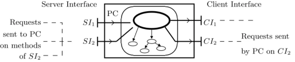
Definition 2 (Primitive Component - Figure 2) A primitive compo-nent is characterized with a compocompo-nent name Name, together with names for
a set of Server Interfaces (SI), and a set of Client Interfaces (CI). We denote by Exported(P C) the set {SIi}i∈1..k and by Imported(P C) the set {CIj}j∈1..l.
P C ::=Name<{SIi}i∈1..k,{CIj}j∈1..l>
Primitive Component Activity: To give functionalities to a PC, we attach to it an ASP term, say a, corresponding to an object to be activated and its dependen-cies (passive objects); the service method of a: srv (the method to be triggered on activation of a; a mapping from SIs to subsets of the served methods; and a mapping from CIs to names of fields of the object a, these fields will store references to components. M ranges over the set of method labels, and L over the set of field labels of a.
P CAct::=NameAct< a, srv, ϕS, ϕC >
where ϕS : Exported(P C) → ℘(M) and
ϕC : Imported(P C) → L are total functions
Server Interface Client Interface
SI1 SI2 CI2 CI1 Requests sent to PC on methods of SI2 Requests sent by PC on CI2 PC
This definition requires that a content P CActis attached to each primitive
component P C, this content consists of a single activity.
Composite components can be built by interconnecting other components – either primitive or composite – and exporting some SIs and CIs.
We suppose that for all components, every interface has a different name (but names could also be disambiguated by using qualified names).
Definition 3 (Composite Component) A composite component is a set of components exporting some server interfaces (εS), some client interfaces (εC),
and connecting some client and server interfaces (defining a partial binding ψ), only interfaces of the direct sub-components can be used:
CC ::=Name¿ C1, . . . , Cm; εS; ψ; εCÀ
Where a component Ciis either a primitive or a composite one: C ::= P C | CC,
and each client interface CI inside CC can only be connected once, leading to the following definition:
εS: Exported(CC) →
[
sc∈C1...Cm
Exported(sc) is a total function ψ: [
sc∈C1...Cm
Imported(sc) → [
sc∈C1,...Cm
Exported(sc) is a partial function εC:
[
sc∈C1...Cm
Imported(sc) → Imported(CC) is a partial surjective function Such that dom(ψ) ∩ dom(εC) = ∅
We define: Exported(CC) = dom(εS) and Imported(CC) = codom(εC).
Defining εS as a function allows to export a given internal server interface as
several external ones, but imposes each incoming request to be communicated to a single destination (each imported interface is bound to a single server interface of an internal component). Similarly, a client interface is exported only once for communications to have a single determinate destination: εC is
a function (each client interface of an internal component is plugged at most once to an exported interface). ψ is a function so that internal communications are determinate too (each client interface of an internal component is plugged at most once to another internal server interface). And finally, also to ensure unicity of communication destination, εC and ψ have disjunct domain so that
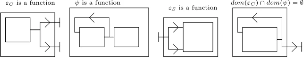
an internal client interface cannot be both bound internally and exported. Correct Connections Figure 3 sums up the possible bindings that are allowed according to Definition 3. The component shown in the figure is a valid CC but not a DCC (DCC will be defined in Section 6.2, Definition 8).
Incorrect Connections Figure 4 shows the impossible bindings that correspond to the restrictions of Definition 3. The condition of Definition 3 that prevents the composition from being correct is written above each sub-figure.
Fig. 3. A composite component
εCis a function dom(εC) ∩ dom(ψ) = ∅
εS is a function
ψis a function
Fig. 4. Incorrect bindings between components
To conclude this section, we present two useful definitions: closed compo-nents that have no interface and form independent systems; and complete com-ponents for which all interfaces are either bound internally or exported: every request sent on a client interface has a destination and every server interface can at some point receive requests.
Definition 4 (Closed Component) A component C is closed if it neither imports nor exports any interface: Imported(C) = ∅ ∧ Exported(C) = ∅ Definition 5 (Complete Component) A primitive component is complete. A composite componentName¿ C1, . . . , Cm; εS; ψ; εC À is complete if it
con-sists of complete components and all its internal interfaces are plugged or ex-ported:
C1, .., Cm are complete component ∧ dom(ψ) ∪ dom(εC) =
[ sc∈C1...Cm Imported(sc) ∧ codom(ψ) ∪ codom(εS) = [ sc∈C1...Cm Exported(sc)
Non-complete components contain unplugged interfaces: some of the CIs of the sub-components must not be used (request without destination) or some of the SIs never receive any request (potential deadlock). As such it is reasonable to forbid them.
4 Example: A Fibonacci Component
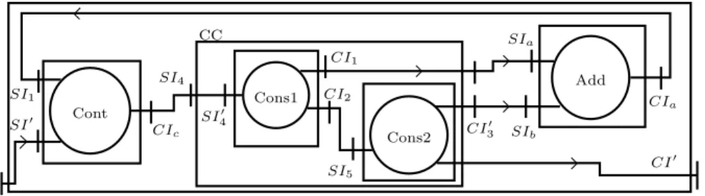
Consider the Process Network that computes the Fibonacci numbers in [19]. Let us write an equivalent composite component as shown in Figure 5. Both Cons1
Add Cons1
Cons2 Cont
ComputeFib(k) send(fib(1))... send(fib(k)) FIB SI1 SI0 SIa SIb SI4 SI5 CI0 3 CI0 CI1 CI2 CIc CIa CC SI0 4 CI: SI:
F IB¿Cont < {SI1, SI0}, {CIc} >,
CC¿ Cons1 < {SI0
4}, {CI1, CI2} >, Cons2 < {SI5}, {CI3, CI 00
} >; {SI4 → SI40}; {CI2 → SI5}; {CI1→ CI10, CI3→ CI30, CI
00
→ CI0
} À, Add <{SIa, SIb}, {CIa} >;
{SI → SI0
}; {CIc→ SI4, CI10→ SIa, CI30→ SIb, CIa→ SI1}; {CI0→ CI} À
AddAct=<[ n1 = 0, n2 = 0, out = [];
serv = ς(s, )Repeat(Serve(set1); Serve(set2); s.out.send(s.n1 + s.n2)), set1 = ς(s, n)s.n1 := n, set2 = ς(s, n)s.n2 := n ],
serv, {SIa→ {set1}, SIb→ {set2}}, {CIa→ out} >
Cons1Act=<[out = [], nxt = [];
serv = ς(s) (out.set1(1); nxt.send(1); Repeat(Serve(send))) , send = ς(s, n)(out.set1(n); nxt.send(n)) ]
serv, {SI0
4→ {send}}, {CI1→ out, CI2→ nxt} >
Fig. 5.A composite component for computing Fibonacci numbers
and Cons2 forward their input to their two client interfaces (upon initialization they respectively send 1 and 0 to their client interfaces); they are merged in a composite component. Add simply sends on its output interface the addition of what the component receives on its two server interfaces. A controller Cont exports a server interface (ComputeF ib(k)) taking an integer k and forwarding k− 1 times its input on the other interface SI1to CIc.
Primitive components for Add and Cons1 are specified by AddAct and
Cons1 Act, the others can be specified similarly (Repeat performs an infinite
loop, “;” expresses sequential composition, both can be expressed directly in ASP). Cons2can be specified by renaming inputs and outputs of Cons1.
Finally, the F IB composite component is built by interconnecting those components as shown and expressed in the figure. For example, requests sent by Cons1 on CI1 are first exported on interface CC10 of CC and then sent,
according to the bindings of F IB, to the interface SIaof Add. Cons2 sends send
5 Translational Semantics
This section gives two possible translational semantics for the component model, with ASP as the target calculus. The first one only instantiates primitive com-ponents and directly binds them but is not compositional. The second one instantiates an additional activity for each primitive and each composite com-ponent, it is defined recursively on the component structure. Both semantics first rely on a deterministic deployment phase; then, components can be started and communicate by asynchronous method calls. Both translations rely on the fact that the names of the interfaces are pairwise distinct, and thus a single component corresponds to each interface.
5.1 A Static Deployment
In the case of a closed component CC = Name¿ C1, . . . , Cm; εS; ψ; εC À, we
define here a translation from this component system into an ASP configuration. We denote C < CC the fact that a component C is inside another one CC:
C <Name¿ C1, . . . , Cm; εS; ψ; εCÀ⇔ ∃i ∈ 1..m, C = Ci ∨ C < Ci
The union of two disjunct partial function is denoted ⊕:
(f ⊕ g)(x) = f (x) if x ∈ dom(f ), g(x) if x ∈ dom(g) else undefined
For each SI of a composite component, ξ returns the primitive component interface which is (recursively) exported to it (Id¯
¯
A is the identity function on
A, C v C0 ⇔ C = C0∨ C < C0). And symmetrically, µ recursively follows
imported interfaces. ξP C= Id ¯ ¯Exported (P C) ξCC: [ CC0vCC Exported(CC0) → [ P C<CC Exported(P C) ξName¿C1,...,Cm;εS;ψ;εCÀ= (ξC1⊕ . . . ⊕ ξCm) ◦ εS Note that, if C is complete then ξC is total
µP C= Id ¯ ¯Imported (P C) µCC: [ P C<CC Imported(P C) → [ CC0vCC Imported(CC0) µName¿C1,...,Cm;εS;ψ;εCÀ= εC◦ (µC1⊕ . . . ⊕ µCm) ΨC defines all the bindings defined inside C:
ΨP C : ∅ → ∅ ΨCC : [ CvCC Imported(C) → [ CvCC Exported(C) ΨName¿C1,...,Cm;εS;ψ;εCÀ= ψ ⊕ ΨC1⊕ . . . ⊕ ΨCm
In the general case, µCand ΨC are partial functions. In the case of a complete
component C, for any client interface CI of C or a component inside C, either µC(CI) or ΨC(CI) is defined.
Φ follows bindings, exportations and importations, to define the bindings between primitive components:
ΦC: [ P CvC Imported(P C) → [ P CvC Exported(P C) ΦC= ξC◦ ΨC◦ µC
For a complete closed component C, ΦC is a total surjective function.
We define below the deployment of the composite component CC: this static deployment creates as many activities as there are primitive components and binds their interfaces accordingly. Let P Cnrange over primitive components
de-fined inside CC: P Cn=Namen<{SIni}i∈1..kn,{CInj}j∈1..ln> s.t. P Cn<CC;
and P CnAct = NamenAct < an, srvn, ϕS n, ϕC n > range over their activities.
We denote Ns(SIp), the index of the primitive component defining the
inter-face SIp: NS(SIni) = n. The term defined in Figure 6 deploys the composite
component CC defined above (the mutually recursive definition of activities let rec . . . and . . . can be built from core ASP terms). This deployment phase does not rely on any request and thus is entirely deterministic.
let rec c1=Active((a1.ϕC 1(CI11) := cNS (ΦCC (CI11))). · · ·.ϕC 1(CI1k1) := cNS (ΦCC (CI1k1 )), srv1)
and c2=Active(a2.ϕC 2(CI21) := cNS (ΦCC (CI21)).· · · .ϕC 1(CI2k2) := cNS (ΦCC (CI2k2 )), srv2)
and . . .
and cn=Active(an.ϕC n(CIn1) := cNS (ΦCC (CIn)).· · · .ϕC n(CInkn) := cNS (ΦCC (CInkn )), srvn)
Fig. 6. Deployment of a composite component
This is sufficient to give a semantics to the components with all useful con-nections bound; but, here, components are not runtime entities and this trans-lation neither is modular, nor gives any way of manipulating dynamically the components (e.g. component reconfiguration is far from trivial). An active ob-ject representation of each composite component will make them accessible and reconfigurable at runtime.
5.2 A Compositional Translation
The compositional translational semantics adds one active object for each com-posite and for each primitive component. This translation does not suppose that any component is closed but requires that method names can be manipulated. During the running phase, requests have to be dispatched between com-ponents: when a PC receives a send request from its contained active object, it serializes this request, forwards a Call request to the destination to which the CI is plugged. Then this method call may go through several CCs (first through CIs and then SIs). Finally, the Call request is received by a PC which de-serializes the request and calls a function on the contained active object. Primitive Components Each PC is translated into a functional active object and a component active object.
The functional active object is built from the object specified in P CAct, but
every ϕC(CIj) field of the active object now references a passive object CIobjj
and requests are sent through this object which acts as a proxy. The CIobjj
serializes (builds a an object containing the method name) each request before forwarding it to the CI interface of the embedding PC (mj methods range over
the method of the interface CI).
CIobjj, [P C = [], ∀mj, mj = ς(s, x)s.P C.send(CIj, mj, x)]
CIobjj allows the component to systematically communicate using the
encap-sulating active object defined below.
The active object for the primitive component contains CIj fields which
store the destination component and interface to which they are plugged. Every request arriving at the CIj interface has to be forwarded to the destination
identified and stored inside the CIj fields Figure 7 shows the object that is
JName <{SIi}i∈1..k,{CIj}j∈1..l> attached to the activity NameAct< a, srv, ϕS, ϕC>K,
let pc= Active(
[∀j ∈ 1..l, CIj= [CDest = [], IDest = []],
started= false, act= [];
∀j ∈ 1..l, setCIj= ς(s, CDest0, IDest0)(s.CIj.CDest:= CDest0).IDest := IDest0,
setact= ς(s, a)s.act := a, start= ς(s)s.started := true, Call= ς(s, SIi, mj, x)s.act.mj(x),
send= ς(s, CIj, mk, x)s.CIj.CDest.Call(s.CIj.Idest, mk, x),
srv= ς(s)Repeat(if started then Serve(Call, send)
else Serve(setCI1..setCIl, setact, start))
] , srv) in
let ao= Active((a.ϕC(CI1):=(CIobj1.P C:= pc) . . .).ϕC(CIl) := (CIobjl.P C:= pc), srv)
in pc.setact(ao); pc
Fig. 7. Primitive Component Deployment
instantiated for each primitive component, note that ao is initialized with the object containing the activity of the component in which ϕC(CIj) fields are
Composite Components Each CC contains the same CI fields as PCs, to-gether with SI fields storing destinations to which received method calls must be forwarded.
For each composite component Name ¿ C1, .., Cm; εS; ψ; εC À, we define
NS0(SIi) the unique number such that CN0
S(SIi)defines the server interface SIi; and similarly N0
C(CIj) such that CN0
C(CIj) is the sub-component containing the client interface CIj. Figure 8 describes the instantiation of a composite
component: it creates an activity for this component, binds the client interfaces according to εC and ψ, and the server interfaces according to εS.
JName¿ C1, .., Cm; ; εS; ψ; εC ÀK,
let c1= JC1K in . . . let cm= JCmK in
letName = Active([
∀SIi∈dom(εS), SIi= [CDest = cN 0S(εS (SIi)), IDest= εS(SIi)],
∀CIj∈codom(εC), CIj= [CDest = [], IDest = []],
started= f alse;
∀CIj∈codom(εC), setCIj= ς(s, Cdst0, Idst0)((s.CIj).CDest := Cdst0).IDest := Idst0,
∀SIi∈dom(εS), setSIi= ς(s, Cdst0, Idst0)((s.SIi).CDest := Cdst0).IDest := Idst0,
Call= ς(s, CI SI, mj, x)s.CI SI.CDest.Call(s.CI SI.IDest, mj, x),
start= ς(s)s.started = true,
srv= ς(s)Repeat(if started then Serve(Call)
else Serve(∀CIj∈dom(εC) setCIj,∀SIi∈dom(εS) setSIi, start))
] , srv) in
∀CIj∈ dom(ψ), cN 0C(CIj ).setCIj(cN 0S(ψ(CIj )), ψ(CIj))
∀CIj∈ dom(εC), cN 0C(CIj ).setCIj(Name, εC(CIj));
c1.start(); . . . ; cm.start(); Name
Fig. 8. Composite Component Deployment
Once deployed, the main component has to be started: JName¿ ... ÀK.start()
The deployment phase relies on setact, and setCI requests but the order of these requests is always the same as first the setact requests are sent during the primitive component creation; and then the setCI are sent by the unique embedding composite component, and thus the deployment phase is determin-istic.
This translation reveals the importance of the first class nature of futures. Indeed, every request transits through several primitive and composite nents; if futures could not be transmitted between activities, then every compo-nent activity would be blocked as soon as a request transits through it, leading almost systematically to a deadlock. Of course, the first class nature of futures is also a major advantage from a functional point of view for both translations. 5.3 Perspective: Reconfiguration and Component Controllers
In the last translation extra activities are added (a kind of component mem-branes), and requests must transit through them. But this additional cost is
counterbalanced by a promising expressiveness: it permits to envision the dy-namic manipulation of components and requests at execution. Indeed, the se-mantics only forwards Call and send requests but it could be extended in order to add non-functional behaviors to components (e.g., fault-tolerance, security), intercept requests, and perform treatments on transiting messages; or reconfig-ure them. Reconfiguration consists in providing primitives allowing to change dynamically εS, εC, or ψ for a given composite; with the last encoding, this can
be realized by convenient calls of setCIj and setSIi methods at the same level
as the reconfiguration occurs. Although very interesting, defining safe and co-herent reconfiguration of a whole distributed component system is a challenging perspective that is beyond the scope of this paper.
6 Deterministic Assembly of Objects and Components
6.1 Static DON
Suppose one has, for each runtime object, a static approximation of the activity it belongs to, denoted ˙α, ˙β, . . .. o ∈ α means o is an object stored in α. Let P art( ˙α) be true if the abstract activity ˙α may dynamically be partitioned into several different activities:
P art( ˙α) ⇔ ∃o, o0, o∈ α, o0 ∈ γ α 6= γ ∧ ˙α = ˙γ
In other words, ∀α, ¬P art( ˙α) iff some abstract activities can be merged to form a single activity at runtime, but no abstract activity is split dynamically. Then, an object which can be either active or passive should be considered statically as active. To summarize:
∀α, ¬P art( ˙α) ⇒ (α 6= γ ⇒ ˙α 6= ˙γ) Moreover, let G(P ) be an approximated call graph:
If a request on the method f oo can be sent from o to o0, and o ∈ ˙α and o0 ∈ ˙β then ( ˙α, ˙β, f oo) ∈ G(P ), which means:
P −→ Q ∧ a∗ αQ = R[ι.f oo(ι
0)] ∧ σ
αQ(ι) = AO(β) ⇒ ( ˙α, ˙β, f oo) ∈ G(P ) Finally, let us characterize Mβ˙P by
∀β, M ∈ Mβ⇒ M ∈ Mβ˙
Then, the following property is an approximation of DON terms:
Definition 6 (Static DON) Suppose the approximation of the set of activi-ties is such that two activiactivi-ties cannot be merged: ∀α, ¬P art( ˙α). A program P is a Static Deterministic Object Network SDON (P ) if for all methods that can be sent at any time from two different activities toward a given destination, those methods cannot interfere:
SDON(P ) ⇔ ( ˙α, ˙β, m1) ∈ G(P ) ( ˙α0, ˙β, m 2) ∈ G(P ) ˙α 6= ˙α0 ⇒ ∀M ∈ Mβ˙P,{m1, m2} 6⊆ M
Theorem 2 (SDON determinism). SDON terms behave deterministically. Proof : It is sufficient to prove that SDON (P ) ⇒ DON (P ), or that
¬DON (P ) ⇒ ¬SDON (P ). Suppose P is not a DON, then it may send in the future two concurrent requests, and thus there is an activity β of a configuration Qsuch that P −→ Q and:∗
∃M ∈ MβP,∃α 6= α 0,∃m 1, m2∈ M,½aα= R[ι.m1(ι 0)] ∧ σ α(ι) = AO(β) aα0 = R[ι2.m2(ι0 2)] ∧ σα0(ι2) = AO(β) Then, as G(P ) is an approximated call graph:
∃M ∈ MβP,∃α 6= α
0,∃m
1, m2∈ MβP( ˙α, ˙β, m1) ∈ G(P ) ∧ ( ˙α
0, ˙β, m
2) ∈ G(P )
and, as ∀α, ¬P art( ˙α), and by definition of Mβ˙P:
∃ ˙α 6= ˙α0∧ ( ˙α, ˙β, m1) ∈ G(P ) ∧ ( ˙α0, ˙β, m
2) ∈ G(P ) ∧ m1, m2∈ M ∧ M ∈ Mβ˙P
Finally, P is not a SDON. 2
Of course, not every DON is a SDON, but SDON can be considered as the best approximation of DON that does not require control flow analysis. 6.2 Deterministic Components
We define a deterministic assemblage of components based on the fact that PCs provide an abstraction for activities and thus the SDON definition can be entirely expressed in terms of specifications of PCs and connections of interfaces. Indeed, suppose that for any two methods of the same SI cannot interfere, then a component system is deterministic if each SI can be accessed by a single activity (that is by a single component). Then, ensuring that only one CI is finally plugged to each SI is sufficient to ensure confluence.
As each PC can be considered as an abstraction of an activity, for each P C, we denote MP C is the potential service of the activity defined by P CAct.
Definition 7 (Deterministic Primitive Component (DPC))
A primitive component P C =Name<{SIi}i∈1..k,{CIj}j∈1..l>is a DPC if its
activity NameAct < a, srv, ϕS, ϕC > associates its server interfaces to disjoint
subsets of the served methods of the embedded active object; and such that two interfering requests necessarily belong to the same SI:
Definition 8 (Deterministic Composite Component (DCC)) A DCC is a composite component built by connecting deterministic components.
DC ::= DCC | DCP
DCC ::=Name¿ DC1, . . . , DCm; εS; ψ; εCÀ
Where each SI is only used once, either bound or exported:
ψ, εC and εS are injective ∧ codom(ψ) ∩ codom(εS) = ∅
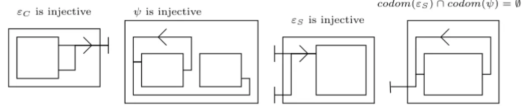
Non-Deterministic Connections Figure 9 illustrates the non-deterministic bind-ings between components, corresponding to restrictions expressed in Defini-tion 8. The condiDefini-tion of DefiniDefini-tion 8 that prevents the composiDefini-tion from being determinate is written above each sub-figure.
εCis injective
codom(εS) ∩ codom(ψ) = ∅
εS is injective
ψis injective
Fig. 9. Non-deterministic bindings between components
A DCC assemblage verifies the SDON property because each DPC statically identifies an activity; and the absence of sharing of SIs ensures that two activities cannot send concurrent requests on the same SI. Finally, the definition for DPC ensures that two requests on different SIs are not interfering.
Theorem 3 (DCC determinism). DCC components behave deterministi-cally.
This theorem relies on the fact that composite components only forward re-quests if necessary, that is to say a request sent by a PC will be directly or indirectly transmitted to the PC that is finally plugged to the concerned in-terface, according to the ΨCC function defined in Section 5.1. In other words,
neither the content nor the order of requests on a given binding is modified by the composite components involved in the communication.
Let us formally prove Theorem 3 in the case of the first translational seman-tics. In the case of the compositional semantics, more intermediate activities are created but each of them still verifies the SDON property.
Proof : Let Φ = ΦCC for CC a DCC. A DCC is only composed of injective
ψ, εC and εS functions, codomains of ψ and εS are disjoint, and domain of ψ
and domain of εC are disjoint, thus the Φ function is injective. In this
PCs (statically defined), thus we can consider PCs as the abstract domain for activities. This abstraction does not merge activities: ∀P C, ¬P art(P C). We de-note comp(SI) the PC such that SI ∈ Exported(P C) and similarly comp(CI) the PC such that CI ∈ Imported(P C). An approximation of G(P ) becomes:
{(P C, P C0, m)|CI ∈ dom(Φ) ∧ P C = comp(CI) ∧ P C0= comp(Φ(CI))
∧ P C0
Act=< a, s, ϕS, ϕC> ∧ m ∈ ϕS(Φ(CI))}
And thus the SDON property is verified (with P C0Act=< a, s, ϕS, ϕC>):
(P C, P C0 , m1) ∈ G(P ) (P C2, P C0, m2) ∈ G(P ) P C6= P C2 9 = ;
⇒ ∀k ∈ 1, 2, mk∈ ϕS(SIk) ∧ P C0= comp(SIk) ∧ SI16=SI2
⇒ ∀M ∈ MP C0,{m1, m2} 6⊆ M
Indeed, m1, m2∈ M and M ∈ MP C0 would imply SI1= SI2 because P C0 is a DPC. Finally a DCC behaves deterministically when deployed with the first
translational semantics. 2
DCC assemblage allows to statically ensure deterministic behavior of com-ponents, only based on the following requirements.
– Potential services can be statically determined, or are statically specified (every served set has been declared as a potential service).
– SI interfaces are respected: they only receive requests on the methods they define; this could be checked by typing techniques [2] on ASP source terms. – Requests follow bindings and are not modified while following these bindings. – There is a bijection between primitive components and functional activities. The two first requirements correspond to static analysis or specification; whereas the two last ones must be guaranteed by the components semantics which is the case for both translational semantics of Section 5.
We have shown in [9] that every Process Network can be translated into a (deterministic) ASP term, which can then be fit into a deterministic assemblage of components. Such a bijection between process networks and DCCs will finally provide a large number of DCCs.
7 Conclusion
This article defines a hierarchical component calculus that provides a very con-venient abstraction of activities and method calls. This abstraction allows static verification of determinism properties. Our component model is aimed at dis-tribution, featuring asynchronous remote method invocations, and futures as generalized references passing through components. Primitive components are defined as a set of Server Interfaces (SI) and client interfaces (CI), together with an ASP term for the primitive component content. Intuitively, each SI corresponds to a set of methods, each CI to a field. Composite components are recursively made of primitives and other composites, with a partial binding between SIs and CIs, and some SIs and CIs exported.
Primitive deterministic components are defined by imposing that each set of interfering requests belongs to the same server interface. A deterministic composite (DCC) avoids potential interferences by imposing at most a single binding towards a server interface. For DCC, both translational semantics lead to configurations that respect the SDON properties, hence their deterministic nature. This results mainly relies on the fact that primitive components provide an abstraction of activities, and interfaces provide an abstraction of potential services.
One might have noticed the absence of any notion of location or machine, in contrast to calculus such as Ambient [8]. Because of the ASP calculus properties, an activity and further a component, can be placed “anywhere” without any semantic consequence. A given hierarchical component can be entirely mapped on a single machine, within the same address space, or fully distributed over the network, each inner component being located alone on its own machine. Ab-stracting activities by components is also convenient for distribution; allowing to map each primitive to a single location and to span composites over several machines.
Two translational semantics for the component model are proposed. The sec-ond translation allows to envision an even more interesting perspective: deter-ministic component reconfiguration. As components and bindings are achieved by ASP active objects, one can imagine to apply the general deterministic prop-erty (DON) to reconfiguration phase and to design coherent reconfigurations.
References
1. Icse ’79: Proceedings of the 4th international conference on software engineering, 1979. Chairman-F. L. Bauer and Chairman-Leon G. Stucki and Chairman-M. M. Lehman.
2. Mart´ın Abadi and Luca Cardelli. A Theory of Objects. Springer-Verlag, New York, 1996.
3. Robert Allen and David Garlan. A formal basis for architectural connection. ACM Transactions on Software Engineering and Methodology, July 1997.
4. Mark Astley and Gul A. Agha. Customization and composition of distributed ob-jects: Middleware abstractions for policy management. In Proceedings of the ACM SIGSOFT 6th International Symposium on Foundations of Software Engineering (FSE), 1998.
5. Fran¸coise Baude, Denis Caromel, and Matthieu Morel. From distributed objects to hierarchical grid components. In International Symposium on Distributed Objects and Applications (DOA), Catania, Sicily, Italy, 3–7 November, LNCS. Springer Verlag, Berlin, Heidelberg, 2003.
6. Philippe Bidinger and Jean-Bernard Stefani. The kell calculus: operational se-mantics and type system. In Proceedings 6th IFIP International Conference on Formal Methods for Open Object-based Distributed Systems (FMOODS 03), Paris, France, 2003.
7. Eric Bruneton, Thierry Coupaye, Matthieu Leclerc, Vivien Quema, and Jean-Bernard Stefani. An open component model and its support in java. In Ivica
Crnkovic, Judith A. Stafford, Heinz W. Schmidt, and Kurt C. Wallnau, editors, CBSE, volume 3054 of Lecture Notes in Computer Science. Springer, 2004. 8. Luca Cardelli and Andrew D. Gordon. Mobile ambients. Theoretical Computer
Science, 240(1):177–213, 2000. An extended abstract appeared in Proceedings of FoSSaCS ’98, pages 140–155.
9. Denis Caromel and Ludovic Henrio. A Theory of Distributed Objects. Springer-Verlag New York, Inc., 2005. To appear.
10. Denis Caromel, Ludovic Henrio, and Bernard Paul Serpette. Asynchronous and deterministic objects. In Proceedings of the 31st ACM SIGACT-SIGPLAN sympo-sium on Principles of programming languages, pages 123–134. ACM Press, 2004. 11. Denis Caromel, Wilfried Klauser, and Julien Vayssi`ere. Towards seamless com-puting and metacomcom-puting in Java. Concurrency: Practice and Experience, 10(11–13):1043–1061, 1998. ProActive available at http://www.inria.fr/oasis/ proactive.
12. Bruneton E., Coupaye T., and Stefani J.B. Recursive and dynamic software com-position with sharing. In Proceedings of the 7th ECOOP International Workshop on Component-Oriented Programming (WCOP’02), 2002.
13. Cormac Flanagan and Matthias Felleisen. The semantics of future and an appli-cation. Journal of Functional Programming, 9(1):1–31, 1999.
14. Dimitra Giannakopoulou, Jeff Kramer, and Shing Chi Cheung. Behaviour analysis of distributed systems using the tracta approach. Automated Software Engg., 6(1), 1999.
15. Andrew D. Gordon, Paul D. Hankin, and Sren B. Lassen. Compilation and equiv-alence of imperative objects. FSTTCS: Foundations of Software Technology and Theoretical Computer Science, 17:74–87, 1997.
16. Robert H. Halstead, Jr. Multilisp: A language for concurrent symbolic compu-tation. ACM Transactions on Programming Languages and Systems (TOPLAS), 7(4):501–538, 1985.
17. Gilles Kahn. The semantics of a simple language for parallel programming. In J. L. Rosenfeld, editor, Information Processing ’74: Proceedings of the IFIP Congress, pages 471–475. North-Holland, New York, 1974.
18. Uwe Nestmann and Martin Steffen. Typing confluence. In Stefania Gnesi and Diego Latella, editors, Proceedings of FMICS’97, pages 77–101. Consiglio Nazionale Ricerche di Pisa, 1997. Also available as report ERCIM-10/97-R052, European Research Consortium for Informatics and Mathematics, 1997.
19. Thomas Parks and David Roberts. Distributed Process Networks in Java. In Proceedings of the International Parallel and Distributed Processing Symposium (IPDPS2003), Nice, France, April 2003.
20. Alan Schmitt and Jean-Bernard Stefani. The kell calculus: A family of higher-order distributed process calculi. Lecture Notes in Computer Science, 3267, Feb 2005.