HAL Id: halshs-00429600
https://halshs.archives-ouvertes.fr/halshs-00429600
Submitted on 3 Nov 2009
HAL is a multi-disciplinary open access
archive for the deposit and dissemination of
sci-entific research documents, whether they are
pub-lished or not. The documents may come from
teaching and research institutions in France or
abroad, or from public or private research centers.
L’archive ouverte pluridisciplinaire HAL, est
destinée au dépôt et à la diffusion de documents
scientifiques de niveau recherche, publiés ou non,
émanant des établissements d’enseignement et de
recherche français ou étrangers, des laboratoires
publics ou privés.
To cite this version:
Eleni Iliopulos. External imbalances and collateral constraints in a two-country world. 2009.
�halshs-00429600�
External imbalances and collateral constraints
in a two-country world
Eleni I
LIOPULOS2009.65
Maison des Sciences Économiques, 106-112 boulevard de L'Hôpital, 75647 Paris Cedex 13
http://ces.univ-paris1.fr/cesdp/CES-docs.htm
External imbalances and collateral constraints in a
two-country world
1;2
Eleni Iliopulos, Paris School of Economics, University of Paris 1
Panthéon-Sorbonne3 and CEPREMAP.
Version: October 14, 2009
1I am very grateful to Guido Ascari, Stefano Bosi, and Tommaso Monacelli for their guidance
and advice. I thank Giancarlo Corsetti, Michel Guillard and Ferhat Mihoubi for useful suggestions; I also thank Gaetano Bloise, Nicola Branzoli, Michel Juillard, Thomas Seegmuller, Tareq Sadeq, Thepthida Sopraseuth, the EPEE and the participants of ZEI and of the Dynare conference at the FED of Boston for interesting discussion. All errors are mine.
2This manuscript is a revision of a chapter of my PhD thesis, (Iliopulos, 2008b).
3PSE, University of Paris 1 Panthéon-Sorbonne, MSE, Bureau 309, 106-112 Bd de L’Hôpital,
Résumé
Cet article étudie la dynamique du compte courant dans le cadre d’une grande économie ouverte, caractérisée par la présence d’agents hétérogènes soumis à des contraintes de crédits ainsi qu’une politique monétaire endogène. Nous incorporons trois caractéristiques-clé largement utilisées dans la littérature concernant la Nou-velle Macroéconomie Ouverte : i) un biais domestique intervenant dans le commerce extérieur, ii) des rigidités de prix, et iii) des biens durables (logements). A…n de limiter la tendance des agents à trop consommer et a…n d’assurer (partiellement) les créanciers contre le risque de défaut, nous incluons des contraintes de collatéral. Nous montrons que le degré d’impatience des agents soumis à des contraintes de collatéral peuvent être à l’origine de déséquilibres extérieurs permanents, notre modèle ayant un unique équilibre caractérisé par un niveau de dette extérieure positif.
Notre modèle nous permet d’analyser le lien existant entre les taux de change, les actifs réels et les ‡ux de capitaux internationaux ce qui nous permettra d’analyser la transmission des chocs ainsi que le rôle de la politique monétaire. Par ailleurs, nous analyserons dans quelle mesure l’évolution du marché de l’immobilier peut a¤ecter le compte courant et la dynamique des taux de change.
Codes JEL: E52, F32, F37, F41.
Mots-clés : Dynamique de la dette extérieure ; dynamique du taux de change réel ; biens durables ; contraintes …nancières ; rigidités de prix ; règles de Taylor.
Abstract
In this article, we focus on current account dynamics in large open economies characterized by debt-constrained heterogeneous agents and endogenous monetary policies. We incorporate three key features that have bulked large in the New Open Macroeconomics literature: i) home bias in trade ii) price rigidities and iii) durable goods (real properties). In order to limit agents’ willingness to consume and to (partially) insure creditors against the risk of default, we incorporate collateral constraints. We show that the impatience of collateral-constrained agents can be at the roots of permanent external imbalances. Indeed our model has a unique and dynamically determinate steady state, which is characterized by a positive level of debt. Our framework allows us to analyze the linkage between exchange rates, real assets and international capital ‡ows. We focus on this mechanism so as to track the (international) transmission of shocks and the implications for the monetary policy. We show how developments hitting the house market can a¤ect current account and exchange rate dynamics.
JEL classi…cation codes: E52, F32, F37, F41.
Keywords: open economy, durable goods, collateral constraints, sticky prices, simple monetary rules.
1. INTRODUCTION
In recent years, agents’ access to credit has been increasingly limited by
col-lateral constraints. The boom4 of collateral constraints is associated to the
devel-opment of housing …nance in several countries. Indeed, during the last 30 years, housing …nance experienced a process of liberalization that introduced more
com-petition and eventually allowed agents to borrow against collaterals.5 Collateral
constraints (partially) insure that in case of default, the creditor can repossess at least (part of) the asset. This is why they are generally associated to better credit conditions for borrowers.
At the same time, the increase in house prices in several countries (together with the development of …nancial intermediation) has encouraged agents to extract equity from the revaluation of their real assets and further borrow against capital gains. This has eventually entailed the expansion of consumption and household debt.
Collateral constraints create a link between the value of real assets and aggre-gate domestic debt; in turn, they create a direct link between ‡uctuations of real asset prices and debt levels. Notice however that spillovers deriving from hous-ing …nance are not only a purely domestic issue. Indeed, thanks to the globalized structure of …nancial markets, intermediaries can convert mortgages into interna-tional assets. Both the development of …nancial intermediation and the boom of collateral constraints have thus reinforced also the link between real assets and the
dynamics of international assets.6 Moreover, since household decisions on housing
purchases are a¤ected by interest rate swings, on the one hand, and international …nancial ‡ows by international returns, on the other, collateral constraints have eventually tightened the mechanism linking real wealth, international capital ‡ows and exchange rates.
The linkage between agents’wealth, exchange rates and the direction of interna-tional capital ‡ows has proved a very powerful mechanism at the roots of …nancial crises in the emerging world. Krugman (1999) studies the link between currency depreciation and the wealth of collateral-constrained …rms in the context of the
Asian crisis.7 He shows that if …rms are collateral constrained and a large share
of their debt is denominated in foreign currency, depreciation has a negative (and dramatic) impact on the wealth of …rms. In turn, as implied by Bernanke and Gertler (1989), the fall in …rms’ wealth, together with debt limits, can lead to a collapse in investments and in aggregate demand.
In our analysis we extend Krugman’s (1999) open-economy "Bernanke-Gertler" e¤ect to a DSGE framework for the analysis of current account dynamics. This mechanism is at the roots of the transmission of various stochastic shocks. We fo-cus in particular on developments a¤ecting agents’wealth (i.e., a¤ecting the housing sector), and their impact on current account and exchange rate dynamics. We track the response of the economy to demand shocks and to the …nancial liberalization
4The share of collateral-constrained agents have increasingly boomed. In US, mortgage debt
has increased from about 60% at the half of the last century to about 90% – including veichles.
5Indeed, housing …nance was a highly regulated sector. For a survey on the developments of
housing …nance, see IMF (2008).
6In Figure 1b we show the trends of current account and house prices for a panel of industrial
countries characterized by signi…cant external imbalances. For those countries, current account de…cits show a co-movement with house prices, in the last decade: increasing current account de…cits (surpluses) are indeed associated to rising (decreasing) house prices.
in housing …nance. Finally, following Ferrero et al. (2008), we analyze the re-sponse of our two-country world to technology shocks; this will provide a deeper
understanding of the mechanisms driving the dynamics of our model.8
The role of collateral constraints has been widely analyzed in a closed econ-omy framework. In presence of durable goods, Kiyotaki and Moore (1997) extend the seminal result of Becker (1980) and Becker and Foias (1987) with discounting heterogeneity to the case of collateral constraints. Their analysis shows that the steady-state level of debt (wealth) of impatient (patient) agents is de…ned by the debt constraint itself; moreover the collateral constraint plays an important role in transmitting the e¤ects of various shocks to other sectors. Indeed, the "…nancial accelerator mechanism" (see Bernanke et al., 1999) ampli…es endogenous devel-opments hitting the credit market. Notice however that when debt contracts are in nominal terms and monetary policy controls interest rates, in‡ation dynamics amplify demand shocks but dampen supply shocks – working thus as a "…nancial decelerator" (see Iacoviello 2005). The reason is that, with nominal debt contracts, an increase in in‡ation has a positive e¤ect on debtors’wealth and a negative one of the wealth of borrowers – with important implications in light of an optimal monetary policy (see Monacelli, 2007).
In an open economy framework, Callegari (2007), Punzi (2007) and Matsuyama
(1990)9 study the linkage between housing and current account dynamics. Since
they do not incorporate nominal prices and exchange rates, there is no scope for them to analyze the role of monetary policy and price rigidities. Analogously, Iacoviello and Minetti (2006) study the interaction between domestic versus foreign borrowing in presence of collateral constraints. None of these works analyzes the above mentioned linkage between exchange rate dynamics, real asset prices and international capital ‡ows.10
In this essay, we extend Iacoviello (2005) and Monacelli (2007, 2008) New-Keynesian framework to a two country-world. This framework is very useful to analyze situations where agents are indebted in equilibrium. We show that, as in Kiyotaki and Moore (1997), discounting heterogeneity and debt limits insure that the collateral constraint is always binding. Moreover, our New-Keynesyan approach allows analyzing trends of nominal variables and the role of monetary policy. Price rigidities and the monetary policy stance could indeed play a role in current account
and exchange rate dynamics.11
Eventually, our world economy is characterized by a positive level of external debt: the stricter collateral constraints, the lower the steady-state level of debt. Clearly, all shocks that a¤ect house prices require adjusting external debt – and thus, a current account adjustment process. Terms of trade play an important role
8Iacoviello and Neri (2008) show that technology shocks and housing demand shocks count for
one quarter each of the cyclical volatility of US housing investment and prices. Moreover, they show how in recent decades demand factors may have played a more prominent role.
9Matsuyama (1990) analyzes the e¤ects of …scal policy shocks on the current account. In his
small-economy setting, an increase in government spending represents a negative income shock for households; it thus dampens their consumption of house services and improves the current account balance. See also ·Iscan (2002) for an empirical analysis on current account and durables.
1 0Caballero and Krishnamurthy (2001) build a model on emerging market crises where they
analyze the interactions between domestic and international collateral constraints on …rms with limited borrowing capacity.
1 1The IMF suggests in this respect that "..given the imperfect global integration of markets
for goods and services and the rigidities that constrain the reallocation of resources to tradable sectors, the redistribution of world spending is likely to require considerable movements in real exchange rates.." (IMF, 2007).
as a transmission channel of country and sector speci…c shocks.
The essay is organized as follows. In Section 2 we introduce our model and in Section 3 we analyze the steady state. In Section 4 we focus on the dynamics follow-ing shocks hittfollow-ing the housfollow-ing market while in Section 5 we analyze the behavior of our model in response to productivity shocks. Section 6 comments the main results of our analysis while the Appendix provides analytical details and Figures.
2. THE MODEL
This model is built on Monacelli (2007, 2008) and Iacoviello (2005) closed economies but is developed in a two-country setting. We consider Home and For-eign respectively (denoted by H and F for simplicity). Both countries are open in every ways but labor. The inhabitants of both countries have same preferences but are heterogeneous in their degree of impatience. More precisely, we assume that the representative inhabitant of country H is more impatient that the one of country F . S/he is not a consumption smoother but her/his desire to consume is limited by a collateral constraint. For simplicity, we will denote the inhabitant of country
H as the borrower and the one of country F as the saver.12
Durable goods (real properties) and tradable goods are produced in a monop-olistic competition framework by domestic and foreign …rms; real properties are non-tradable goods and can be used as collateral. Think for instance of houses:
leaving tourism a part, houses are generally owned by and sold to residents.13
Goods are then purchased and sold to …nal consumers by domestic retailers, in a competitive environment. The representative retailer in the housing sector in coun-try H (in councoun-try F ), buys Home (Foreign)-produced durables only and sell them to …nal consumers in country H (country F ) only. Analogously, the representative retailer in the tradable sector, buys both Home and Foreign-produced goods to sell them to …nal consumers in the Home (Foreign) country only. Final consumers enjoy services deriving from durables and consume tradable goods. Finally, agents can smooth their consumption by exchanging securities on international incomplete markets; debt in country H is subject to a collateral constraint.
2.1. Retailers
We suppose that intermediate goods are sold in both countries to …nal consumers by an in…nite set of retailers operating in a competitive environment. Goods mar-kets in each country are segmented into the tradable and real properties sector. We will denote by j = T , the representative retailer operating in the tradable sector; j = n, the representative retailer operating in the durable sector (real properties). The retailer j = T in country H (in country F ) buys Home and Foreign-produced tradables and sell them to the Home (Foreign) market. The retailer j = n buys real properties produced in country H (country F ) and sell them to the Home (Foreign) market.
2.1.1. Tradables
Consider …rst the case of the retailer operating in the tradable sector in country H. S/he has access to both domestic and foreign-produced goods and sell them
1 2Notice however that this will be an endogenous result of the model. 1 3See also Engel and Wang (2008) for some discussion.
to H …nal consumers only. In order to re‡ect consumer’s preferences, we assume
that the behavior of retailers is a¤ected by home bias.14 Retailers operate in a
perfectly competitive environment and their basket of production is the following CES bundle: YT ;t= 1 Y 1 h;t + (1 ) 1 Y 1 f;t 1
where represents the weight of Home produced goods in consumers’bundles (in
presence of home bias, > 0:5) and > 0 is the elasticity of substitution between
Home and Foreign produced goods. For simplicity, from now on we denote all variables referred to Home (Foreign) goods with the index h (index f ). Retailers’ demand for respectively Home and Foreign produced goods is the result of an optimization problem. The CES-related price index of tradables is:
PT ;t= h Ph;t1 + (1 ) Pf;t1 i 1 1 (1) Retailers’intermediate demand for Home produced and Foreign produced goods (Yh;t and Yf;t; respectively) is:
Yh;t = YT ;t Ph;t PT ;t (2) Yf;t = (1 ) YT ;t Pf;t PT ;t (3) In country F; retailers in the tradable sector behave symmetrically. This implies that the weight of Foreign produced goods on country F CES production bundle
is the same as the one of Home produced goods in country H15, i.e.:
YT ;t= (1 )1 Y 1 h;t + 1 Y 1 f;t 1 (4) Pro…t maximization implies that retailers’intermediate demand for foreign and domestic goods respectively in country F is:
Yh;t = (1 ) YT ;t Ph;t PT ;t ! (5) Yf;t = YT ;t Pf;t PT ;t ! (6) Notice however that retailers also need to choose amongst the di¤erent (in…nite) varieties of domestic and foreign goods, i. We suppose that the Home (Foreign)-produced basket of the representative retailer is in turn a CES bundle of a contin-uum of in…nite varieties of goods, i. Retailers’ intermediate demand for a single variety of Home produced (Foreign) good is thus:
1 4An alternative way to introduce home bias in our model would be to leave the choice between
domestically-produced versus foreign-produced goods to consumers.
1 5The corresponding price index is: P T ;t=
h
(1 ) Ph;t1 + Pf;t1 i
1 1
Yh;t(i) = Yh;t Ph;t(i) Ph;t " (7) Yf;t(i) = Yf;t Pf;t(i) Ph;t " (8) where " > 116; " > : Analogously, in the rest of the world:
Yh;t(i) = Yh;t Ph;t(i) Ph;t ! " (9) Yf;t(i) = Yf;t Pf;t(i) Pf;t ! " (10) 2.1.2. Durables
Consider now the housing sector. The representative retailer in country H chooses a set of houses amongst an in…nite continuum of domestically produced real properties. Her/his demand for each di¤erentiated good, i, is the result of
pro…t maximization in a competitive environment17, i.e.:
Yn;t(i) =
Pn;t(i)
Pn;t "
Yn;t (11)
where " is the elasticity of substitution between single goods, i :18 Analogously, in
the Foreign country, the intermediate demand for real properties of the representa-tive retailer is:
Yn;t(i) = Pn;t(i) Pn;t
"
Yn;t (12)
2.2. Optimal consumption in country H
Consider now the representative inhabitant of country H. His/her utility is a
positive function of her/his basket of consumption, Ct and a negative function of
her/his labor supply, Nt i.e.19:
max E0 ( X t=0 tU (C t; Nt) )
1 6In order to keep countries H and F as symmetric as possible, we assume identical elasticities
of substitution across countries.
1 7Where the CES production bundle of the retailer is: Y n;t 0 @ 1 Z 0 Yn;t(i) " 1 " di 1 A " " 1 :The
associated price index is: Pn;t
0 @ 1 Z 0 Pnj;t(i)1 "di 1 A 1 1 "
1 8For simplicity, we assume that the elasticity of substitution between the in…nite varieties of
Home (Foreign) produced goods is the same for both sectors.
1 9In our economy all agents have same preferences and maximize a generic utility
func-tion. In the numerical simulations we will consider the following functional form: Ut =
where is the borrower’s discount factor. We do not introduce explicitly money in the utility function and we use it as the numéraire of our cashless economy à la Woodford.
The representative borrower consumes a bundle that is a CES composite of tradables and services deriving from the stock of real properties. For simplicity, we assume that agents start enjoying services deriving from durables in the same period they purchase them and are proportional to the stock of houses. We also
assume that agents cannot rent/lend houses.20 The borrower consumption basket
is thus: Ct= h 1 C 1 T ;t + (1 ) 1 C 1 n;t i 1
where is the weight of tradables in the basket and > 0 is the elasticity of
substitution between durable services and tradables. The following assumption on preferences always needs to hold in both countries:
Assumption 1 (preferences) Uk 2 C2, UkC > 0, UkN < 0, UkCC < 0,
UkCCUkN N > UkCN2 for every (Ck; Nk) such that Ck; Nk > 0, k =borrower; saver.
Also, Inada conditions for consumption hold.
The individual budget constraint in real terms of tradable consumption is21:
CT ;t+ xt(Cn;t (1 ) Cn;t 1) + Rt 1 bt 1 T ;t bt+ WtNt PT ;t +X PT ;t (13)
where CT ;trepresents tradable consumption, Pn;t(Cn;t (1 ) Cn;t 1) is the cost
of durable expenditure in period t; b are net external liabilities in real terms of
tradable consumption22, where B D qD are net external liabilities in
nom-inal terms, D are home-currency domestic securities, q is the nomnom-inal price of Foreign currency in terms of Home currency and D are foreign-currency Foreign
securities23. Notice also that x
t PPn;tT ;t is the relative price of real properties
and T ;t PPT ;tT ;t1 is the aggregate in‡ation rate in the tradable sector24: In
prac-tice, in each period the borrower buys tradables, CT; and real properties; s/he pays
the debt service on her/his debt, where R is the gross nominal interest rate factor. S/he enjoys resources coming from foreign borrowing, B; labor income, W N and
pro…ts, coming from their …rms (operating in a monopolistic competition
frame-work). Labor is assumed mobile across sectors but not across countries; therefore, the wage is the same in each sector but not necessarily in each country.
2 0This implies that CPI in‡ation corresponds to aggregate in‡ation in the tradable goods sector. 2 1The individual budget constraint in nominal terms is:
PT ;tCT ;t+ Pn;t(Cn;t (1 ) Cn;t 1) + Rt 1Bt 1
Bt+ WtNt+
X
The budget constraint is assumed to hold with equality around the deterministic steady state.
2 2Notice that b t 1=
Bt 1
PT ;t 1
2 3See the Appendix for all details concerning the optimization program of the consumer. 2 4The in‡ation rate in the durable sector is de…ned as
n;t Pn;t
Pn;t 1, while h;t
Ph;t
Borrowers’ capacity to obtain credit is limited by a collateral constraint. We suppose that households’ debt is constrained to be a share of the value of their durables (real properties), and debt contracts are issued in nominal terms, i.e.:
bt (1 ) Cn;txt (14)
where is the fraction of durables that cannot be used as a collateral and can be
interpreted as the inverse of the loan-to-value ratio: the larger , the more stringent
the constraint. For simplicity, we assume to be an exogenous parameter of our
model. The role of collateral constraints and the implications of their structure has been recently analyzed in a New-Keynesian framework by Calza et al. (2006)
in a closed economy framework.25 Eventually, collateral constraints allow agents a
better access to credit. Indeed, they partially ensure the creditor against the risk of
default: in case of default, the creditor can always repossess (part of) the asset.26
In our two-country world, constraint (14) reduces to a limit on international borrowing. This should not surprise the reader. Since we aim at analyzing current account dynamics, we are interested in the behavior of aggregate variables, and in the dynamics of ‡ows (of goods and …nancial capital) between countries. In aggre-gate, the sum of domestically traded assets and liabilities in each country is equal to zero. Thus, if indebted, our representative agent of each country cannot but be indebted towards his foreign counterpart only. Indeed, thanks to the globalized structure of …nancial systems, mortgages can be easily converted into international assets. Our representative agent in each country can thus act as a …nancial in-termediary and sold her/his (collateralized) debt abroad. In this vein, collateral constraints (and their impact) are transferred to an international dimension.
Notice …nally that (14) implies also that an increase in the relative price of real properties allows agents to increase their level of debt.
The …rst order conditions of borrowers’optimization program are: UN;t UT ;t = Wt PT ;t (15) xtUT ;t = Un;t+ (1 ) EtfUT ;t+1xt+1g + UT ;t t(1 ) xt (16) t = 1 Et Rt T ;t+1 UT ;t+1 UT ;t (17) Equation (15) represents a standard consumption/leisure arbitrage. Equation (16) represents the intertemporal demand for tradable consumption relatively to durables. In equilibrium, the value of the utility deriving to the borrower from present consumption of tradables needs to equal the value of direct utility deriving from the direct housing services plus the value of their indirect utility, i.e.: i) the utility deriving from the possibility of selling real properties and buying durable
consumption in future, (1 ) EtfUT ;t+1xt+1g and ii) the marginal utility
stem-ming from relaxing the collateral constraint, and consustem-ming additional non-durable goods, UT ;t t(1 ) xt:
Equation (17) represents a modi…ed Euler equation for country H –where t t
is the Lagrangian multiplier associated to the collateral constraint and t the one
2 5For more discussion see also Monacelli (2007, 2008), Iacoviello (2005) and Campbell and
Hercowitz (2006).
2 6In Bernanke and Gertler (1989) they are justi…ed by the presence of private information and
limited liability. In Kiyotaki and Moore (1997) they are the response to problems of enforcing contracts.
associated to the budget constraint. Clearly, it reduces to the standard Euler
equation whenever t =0. If t > 0, the marginal utility of current
consump-tion exceeds the gain of shifting intertemporally one unit of consumpconsump-tion (savings): UT ;t > Et
n
Rt
T ;t+1UT ;t+1
o
. If this is the case in each period, the representative agent in country H is not a consumption smoother and …nances current consump-tion with as much credit as s/he can have access to (i.e., the collateral constraint
is binding). Clearly, talso represents the marginal value of additional debt27: by
marginally relaxing the collateral constraint one can have access to more current consumption.
Finally, one can rewrite (16) as: Un;t UT ;t = xt(1 t(1 )) (1 ) Et UT ;t+1 UT ;t xt+1 (18)
Notice that the RHS of equation (18) represents the user cost of durables in terms of non-durables at time t. It represents the price you pay for the ‡ow of consumption services from durables during the period; the cost is obviously a positive function of
the interest rate and the relative price of durables (for t…xed). By substituting
(17) in (18) and log-linearizing (18), it is possible to isolate the e¤ect of on the user cost, during the dynamics around the steady state, as shown in the Appendix (its impact on the steady state is also discussed in the Appendix). The impact of a variation in on the user cost crucially depends both on the structure of the collateral constraint and the parametrization. In our framework, it is generally negative. This implies that a decrease in the marginal utility of borrowing makes
houses less useful and entails a substitution e¤ect in favour of tradables.28
2.3. Exchange rates and terms of trade
In presence of home bias, the law on one price only holds for the single basket of Foreign produced and Home produced tradables, separately. In practice:
Ph;t= qtPh;t
and
Pf;t = qtPf;t
where q is the nominal exchange rate (the Home-currency price of Foreign currency)
and > 1
2 implies PT ;t6= qtPT ;t:
In addition, in equilibrium, the following relationship between Home and Foreign net external liabilities always needs to hold:
Bt= qtBt (19)
where B is Home-currency net external debt in nominal terms and B 29 are lenders’
net external assets in Foreign currency. Obviously, if B > 0 borrowers are net debtor and savers are net lenders.
2 7 can also be interpreted as the price of an asset; indeed, it is tied to a payo¤ that depends
on the deviation from the Euler equation – see Monacelli (2007).
2 8Having said that, for very small depreciation rates, we recover Monacelli (2008) result in
presence of a (slightly) di¤erent collateral constraint. See the Appendix.
2 9Clearly, B =D q D
In our two-country simple world, houses cannot be rent. This implies that the
CPI price index coincides with the aggregate price index of tradable goods, PT :30
It is thus straightforward to calculate the CPI real exchange rate of country H as:
t= qt
PT ;t PT ;t
For simplicity, from now on when referring to the real exchange rate of H; we
will consider the CPI based real exchange rate.31 Notice …nally that in absence of
home bias, the CPI-based real exchange rate is constant in all periods; this would certainly be at odds with reality (see Figure 1a).
We …nally introduce country H terms of trade and we de…ne them in the fol-lowing way: St= Pf;t Ph;t = Pf;t Ph;t (20)
Symmetrically, country F terms of trade are thus: St = Ph;t Pf;t = Ph;t Pf;t = S 1 t
The bond market-clearing condition (19) can be rewritten as a function of terms of trade, i.e.: bt = bt (1 ) St1 + St1 + 1 ! 1 1 (21)
2.4. Optimal consumption in country F
We consider now the representative agent of country F . We suppose that agents in country F are more patient than agents in country H. Thus, the discount rate of the borrower is strictly lower than the one of country F representative agent (the saver). Savers maximizes the following utility function:
max E0 ( X t=0 tU (C t; Nt) )
where is their discount factor, Nt is labor e¤ort and Ct is a CES composite
good of tradables and services arising from durables. For simplicity, from now on, all variables referring to the foreign country (and currency) will be indexed by an asterisk.
Assumption 2 always holds:
Assumption 2 (discounting) ; 2 (0; 1) ; < :
3 0Indeed, the CPI basket does not include the price of houses.
3 1Analogously, in presence of durable goods, Engel and Wang (2008) build a non-utility based
consumption price index. This index is calculated as a weighted average of di¤erent prices subindexes and is used to compute the real exchange rate of their economy.
Assumption 2 is crucial in explaining external debt dynamics in our model; it
is not new in international …nance.32 Ghironi et al. (2005) introduce
heteroge-neous discounting in an overlapping generation framework33. More recently, Choi
et al. (2008) track the dynamics of US current account introducing endogenous heterogeneous discounting.
Savers’consumption basket is composed as the one of borrowers, i.e.:
Ct =h 1C 1 T ;t + (1 ) 1 C 1 n;t i 1
where Cn are services deriving from real properties in the Foreign country and CT
is a basket of tradables. The budget constraint of the F -agent in real terms of
tradable consumption is34: CT ;t+ xt Cn;t (1 ) Cn;t 1 Rt 1bt 1 T ;t bt+WtNt PT ;t + X i PT ;t (22)
where Wt are foreign-currency wages in the Foreign country, R are nominal
in-terest rates in the Foreign country and are pro…ts. Finally, B D
q D are
Foreign net external assets in Foreign currency and bt are net external assets in
real terms of tradables. Finally, we introduce a no-Ponzi game condition on net international assets35: lim i!1Et bt+i i Y z=1 Rz 0 (23)
The …rst order conditions of savers’optimization program are: UN;t UT ;t = Wt PT ;t (24) UT ;txt = Un;t+ (1 ) Et xt+1UT ;t+1 (25) UT ;t = Et ( UT ;t+1 Rt T ;t+1 ) (26) Equation (24) states the standard arbitrage condition between leisure and con-sumption and equation (25) is the intertemporal demand equation for durables versus nondurable goods. Equation (26) is a standard Euler equation.
Finally, we need to introduce the relation linking interest rates in country H and in country F . In order to obtain it, we substitute for gross external assets and
liabilities in the budget constraint of country H or F (remember that B D qD ).
Rewriting the budget constraint in real terms of tradable consumption and re-calculating the …rst order conditions for the borrower and/or the lender, one can easily …nd the needed condition. It is possible to show (see the Appendix for all details) that the following modi…ed uncovered interest parity condition needs to hold:
3 2Our hypothesis is also consistent with Masson et al. (1994) and Henriksen (2002) who relate
current account dynamics with demographic factors. Analogously, Chinn and Prasad (2000) …nd that demographic factors are signi…cant determinant of the current account balance.
3 3For more discussion, see also Buiter (1981) and Weil (1989). 3 4It holds with equality around a deterministic steady state.
3 5This condition does not bind. Analogously, given lenders’ relative patience, any collateral
Rt= Et
qt+1
qt
Rt (27)
The absence of arbitrage possibilities between domestic and foreign assets im-plies that the marginal utility of investing in Home assets is equal to the one agents obtain by investing in Foreign assets. Notice …nally that given the stochastic setup of our framework and the assumption of incomplete markets, the uncovered interest parity condition only holds in expectations.
2.5. Production
We now set the structure of production in our two-country world. For simplicity we suppose that labor is homogeneous and mobile across sectors in the same country –but not around the world. We assume also that the representative agent in each country is also the owner of representative …rms in each country. Markets in each country are segmented into tradables and durables (real properties). Firms in both sectors operate in a monopolistic competition environment and are characterized by the good they produce.
Real properties’producers at Home (in the Foreign country) only sell their goods to Home (Foreign) markets while tradables’producers sell them to retailers of both countries. We suppose that there are i …rms producing i non perfectly substitutable durables (tradable goods). Each …rm is characterized by a production function F ,
which depends on labor, Nland a productivity shifter Al, which is common for all
…rms within the same sector, l = h; n (f; n). The following proposition needs to hold:
Assumption 3 (technology): F is homogeneous of degree 1 with F 2
C2; F
N > 0; FN N 0: Moreover F (0) = 0; limN!0F0(N ) = +1; limN!1F0(N ) =
0:
2.5.1. Tradables
We …rst focus the attention on the tradable sector in country H. Firm i pro-duction function is consistent with Assumption 3 and is de…ned for simplicity as:
Fi;t(Nh;t(i)) = Ah;tNh;t(i)
Firms maximize the pro…t function: E0
(1
X
t=0
0;t Fi;t(Nh;t(i))Ph;t(i) WtNh;t(i)
!T 2 Ph;t(i) Ph;t 1(i) 1 2 Ph;t !)
given retailers’ demand functions. is the borrower’s stochastic discount factor
and: t;t+1 0;t+1 0;t Et 1 1 t t+1 t PT ;t PT ;t+1
where is the borrower’s Lagrangian multiplier (i.e., the marginal utility of income)
!T 2 Ph;t(i) Ph;t 1(i) 1 2 Ph;t
are the …rm’s costs associated to adjusting prices (menu costs); following Rotemberg and Woodford (1997), we assume that adjustment costs are quadratic. In practice, each period …rms need to optimally balance the costs arising from resetting prices and the costs associated to deviating from optimality.
Analogously, the stochastic discount factor of …rms in country F is:
t;t+1 0;t+1 0;t Et ( t+1 t PT ;t PT ;t+1 )
where is lenders’stochastic discount factor and is the Lagrangian multiplier
associated to the saver’s budget constraint.
In both countries …rms choose their optimal sequence fNh;t(i) ; Ph;t(i)g,
n
Nf;t(i) ; Pf;t(i)o : Nominal and real marginal costs in H (M C and mc, respectively) are:
M Ch;t = Wt Ah;t mch;t = Wt Ph;tAh;t (28)
In a symmetric equilibrium: Ph;t(i) = Ph;t: We can thus simply solve for optimal
prices. We obtain the following New Keynesian Phillips Curve (NKPC): !T( h;t 1) h;t= Fh;t(Nh;t) " (1 ") " + mch;t +!T Et 8 < : 1 1 t UT ;t+1 UT ;t " + (1 ) St1 + (1 ) St+11 # 1 1 ( h;t+1 1) h;t+1 9 = ; The standard optimization program of the representative agent implies that in equilibrium there cannot be gains in exchanging leisure with consumption; the non-arbitrage condition leisure/consumption (15) needs to hold. Condition (15) can be here rewritten as:
UN;t UT ;t = Wt Ph;t h + (1 ) St1 i 1 1
therefore, when we substitute it in (28), we obtain:
mch;t= 1 Ah;t UN;t UT ;t h + (1 ) S1t i 1 1 (29) Clearly, terms of trade a¤ects the Phillips curve both in the form of the marginal cost, and through the discount factor. By incorporating (29) and the relation Fh;t(Nh;t) = Ah;tNh;tin the above Phillips curve, we obtain:
!T( h;t 1) h;t= Ah;tNh;t" (1 ") " + 1 Ah;t UN;t UT ;t + (1 ) St1 1 1 (30)
+!T Et 8 < : 1 1 t UT ;t+1 UT ;t " + (1 ) St1 + (1 ) St+11 # 1 1 ( h;t+1 1) h;t+1 9 = ; Without price rigidities, the real marginal cost is constant at the mark-up. Notice also that in the tradable sector, terms of trade create a wedge between the rate of substitution between consumption and leisure on the one hand, and the marginal product of labor on the other. The real marginal cost is directly a¤ected by movements in terms of trade. This creates a scope for policy intervention whenever the policy-maker aims at optimal policies (for some discussion see Faia and Monacelli, 2008).
Analogous considerations apply for country F . Marginal costs are:
mcf;t= 1 Af;t UN;t UT ;t h + (1 ) St 1+ i 1 1 (31) and the NKPC is:
!T f;t 1 f;t= Af;tNf;t" " (1 ") " + + (1 ) S 1+ t 1 1 UN;t Af;tUT ;t # (32) +!T Et 8 < : UT ;t+1 UT ;t " + (1 ) St1+ + (1 ) St+11+ # 1 1 f;t+1 1 f;t+1 9 = ; 2.5.2. Durables
The price dynamics in the housing sector can be easily individuated by following
the same lines of the previous section. The New Keynesian Phillips curve for
durables (real properties) is:
!n( n;t 1) n;t = An;tNn;t" (1 ") " + mcn;t + !n Et 1 1 t 0;t+1 0;t ( n;t+1 1) n;t+1 Pn;t+1 Pn;t where, again: t;t+1= 0;t+1 0;t = Et 1 1 t t+1 t PT ;t PT ;t+1 and thus: !n( n;t 1) n;t = An;tNn;t" (1 ") " + mcn;t + !n Et 1 1 t UT ;t+1 UT ;t xt+1 xt ( n;t+1 1) n;t+1
Also, given the arbitrage consumption-leisure, we can rewrite …rms’marginal costs in the housing sector as:
mcn;t= 1 An;txt UN;t UT ;t (33)
Notice that there is a wedge between the ratio of marginal utilities and the marginal cost. This wedge is created by a variation in the relative price, x. When the monetary authority aims at implementing an optimal policy, the presence of this wedge leaves the policy maker a scope for policy intervention (for some discussion see Monacelli, 2007).
Incorporating (33) in the above New-Keynesian Phillips curve, we obtain: !n( n;t 1) n;t = An;tNn;t" (1 ") " + 1 xt UN;t UT ;tAn;t (34) +!n Et 1 1 t UT ;t+1 UT ;t xt+1 xt ( n;t+1 1) n;t+1
Analogously, the NKPC in country F is:
!n n;t 1 n;t = An;tNn;t" " (1 ") " + 1 xt UN;t UT ;tAn;t # (35) +!n Et ( UT ;t+1 UT ;t xt+1 xt n;t+1 1 n;t+1 )
where real marginal costs are:
mcn;t=
1 xt
UN;t
UT ;tAn;t (36)
Notice that we have a priori allowed for the possibility of price rigidities in the housing sector. Having said that, we will reasonably assume in our benchmark
simulations that house prices are not rigid. Indeed, as Iacoviello and Neri (2008)36
remark, most houses are priced for the …rst time when they are sold. Moreover, since each house is a very expensive good, in case menu costs had a signi…cant …xed
component, the incentive to renegotiate its price would predominate. 37
2.6. Market clearing
2.6.1. Home country
For markets to be cleared in country H; total purchases of real properties need to equal the total domestic production; they also need to account for the costs of price rigidities. We remind the reader that in this model real properties are non-tradable goods. Thus:
An;tNn;t= Cn;t (1 ) Cn;t 1+
!n
2 ( n;t 1)
2
Given that labor is not mobile across countries, labor market clearing implies:
Nn;t+ Nh;t= Nt (37) Therefore: An;tNn;t= Cn;t (1 ) Cn;t 1+ !n 2 ( n;t 1) 2 (38)
3 6See also Barsky, House and Kimball (2007).
3 7Our simpli…ed framework does not allow to model phenomena related to asset prices bubbles.
Focus now on the Home sector of tradables. Market clearing requires: Ah;tNh;t= Ch;t+ Ch;t+
!
2 ( h;t 1)
2
where Ch and Ch are consumption levels of Home tradables at Home and in the
Foreign country, respectively. Notice that local retailers of tradables in country H operate in a perfectly competitive environment and only sell their products to Home inhabitants (in practice, they simply act as aggregators). Therefore, the market of Home-produced tradables clears when the total amount of produced goods equals
the aggregate demand of retailers. In practice, Ch;t = Yh;t; Ch;t = Yh;t; CT ;t =
YT ;t: Recalling that retailers’demand for domestically and foreign produced goods
are respectively, Yh;t= YT ;t PPh;tt;t and Yf;t= (1 ) YT ;t PPf;tt;t the market
clearing condition for the tradable sector can be rewritten …rst as:
Ah;tNh;t= YT ;t Ph;t PT ;t + (1 ) YT ;t Ph;t PT ;t ! +! 2 ( h;t 1) 2
and then as a function of terms of trade, i.e.:
Ah;tNh;t = Ct;t h + (1 ) St1 i1 (39) + (1 ) Ct;th(1 ) + St1 i1 +!T 2 ( h;t 1) 2 2.6.2. Country F
Given the symmetric structure of our world economy, market clearing conditions for country F have a symmetric structure to that of country H: Market clearing conditions for country F are listed in the following.
Labor market clearing requires:
Nn;t+ Nf;t= Nt (40)
Market clearing in the non-tradable sector requires: An;tNn;t= Cn;t (1 ) Cn;t 1+!n
2 n;t 1
2
(41) Finally, market clearing in the tradable sector implies:
Af;tNf;t = (1 ) CT ;t h St 1+ (1 )i1 (42) + CT ;thSt 1(1 ) + i1 +! 2 f;t 1 2
2.6.3. Budget constraints and current account
If monopolistic …rms are owned by the inhabitants of the country in which they are located, the resources-expenditure balance of the borrower is given by the budget constraint (13), holding with equality around a deterministic steady state. Therefore, by substituting for real pro…ts and for (39) and (38) in the borrower’s
budget constraint, the resource constraint of the representative agent in country H is: (1 ) CT ;tS 1 t + (1 ) St1 (1 ) CT ;t h 1 + St1 i1 h + (1 ) St1 i 1 1 (43) = bt Rt 1 bt 1 T ;t
Equation (43) shows that the in‡ows of foreign resources net of interest payments (the RHS) needs to equalize the consumption of tradables at Home, net of Foreign
consumption of tradables (weighted for terms of trade). Equation (43) is also
the current account equation for country H. More explicitly, we de…ne the current account of country H (in real terms of home tradable consumption) as the variation
of home-currency assets (in real terms of tradable consumption)38, i.e.:
cat = bt 1 T ;t bt (44) cat = xtAn;tNn;t+ Ah;tNh;t Ph;t PT ;t CT ;t xt(Cn;t (1 ) Cn;t 1) (45) bt 1 T ;t (Rt 1 1) 1 PT ;t h Pn;t ! 2 ( n;t 1) 2 + Ph;t ! 2 ( h;t 1) 2i
Clearly, by substituting An;tNn;t and Ah;tNh;twith (38) and (39) and equating (44)
and (45) we obtain equation (43).
In the rest of the world, the corresponding resource constraint is:
CT ;t S 1 t (1 ) h St 1(1 ) + i Rt 1 bt 1 T ;t 1 (46) = bt+ (1 ) CT ;t h St 1+ (1 )i1 h (1 ) St 1+ i 1 1
Equation (46) can be also interpreted as a current account equation of country F .
2.7. Monetary policy
The recent house prices boom and the prospect of a global downturn as a con-sequence of sharp softening in housing sectors have triggered a debate on wether policy makers should respond to house prices. Conventional mainstreams agree that central bankers should respond to asset price changes only when they a¤ect in‡ation, output and expectations (Mishkin, 2007). However, there are "bene…ts to be derived from leaning against the wind...(and)..increas(e) interest rates to stem
the growth of house price bubbles and help restrain the building of …nancial imbal-ances" (IMF, 2008).39
There is also a general agreement on the desiderability to target in‡ation only
in the sectors where prices are stickiest.40 In this light, by letting prices free to
move in the ‡exible-prices sectors, the monetary authority avoids output swings in the sticky-price sectors to stabilize the overall price index.
While refraining from normative issues, we limit our analysis to the e¤ects of stochastic shocks in presence of alternative policy stances. In our framework, we as-sume that exchange rates are completely ‡exible and policy makers do not engage in any speci…c exchange rate policy. This leaves the central bank three possi-ble targets: durapossi-ble goods in‡ation, tradapossi-ble goods in‡ation and/or domestically-produced tradables’ in‡ation. In the following, when focusing on the response of the economy to shocks, we will track the adjustment dynamics with di¤erent Taylor rules.
In our simpli…ed exercise, we assume that the policy maker does not aim to stabilize output. Clearly, as remarked by Iacoviello (2005) in a similar framework, output targeting may be a source of possible policy trade-o¤s. For the moment we suppose that each policy maker react both to durables’ and home-produced tradables’in‡ation according to the following Taylor rules:
Rt R = h;t h 1;h n;t n 2;h (47) Rt R = f;t f ! 1;f n;t n 2;f (48)
In a two country setup, nominal determinacy requires 1 and/or 2 to be
su¢ ciently large; we assume that the monetary policy is set so as to ensure su¢ cient conditions for nominal determinacy (see Benigno and Benigno, 2000). Notice …nally that the above simple rules are not e¢ cient: any change a¤ecting the natural interest rates will likely entail an in‡ationary/de‡ationary bias.
2.8. Equilibrium conditions
For each monetary policy in country H and F , the equilibrium of our world economy is de…ned by (13) and (14) holding with equality around the deterministic steady state (see discussion in the following section), (15), (16),(25), (24), (26),
(17), (27) and the no-Ponzi game condition, (23)41. In the tradable production
sector, (30) and (32) need to hold while in the durables production sector (34) and (35). Market clearing is insured by (37)-(43) and (19). Finally purchasing parity conditions need to hold.
3. STEADY STATE
In this section we focus on the qualitative features and the dynamic proper-ties of the steady state. Once we have proved the existence of a "well behaving
3 9For more discussion on house prices and monetary policy targets see Borio and White (2004),
Bordo and Jeanne (2002).
4 0See Aoki (2001) and Benigno (2004).
equilibrium", it is possible compute it analytically (see the Appendix).
3.1. Dynamic properties of the steady state
In order to show the existence of a determinate steady state and on its features we …rst shift our attention to the (modi…ed) steady-state Euler equations of our model.
Consider …rst equations (26) and (58) –see the Appendix –at the steady state.
Notice also that in steady state, T = T (where is the steady-state depreciation
rate of the nominal exchange rate). Indeed terms of trade are …xed in steady state. Also, long-run values of tradable in‡ation coincide with the target of the monetary policy for tradables in the Home and in the Foreign country, respectively. We can thus pin down the long-run value of ; i.e.:
= 1 (49)
implying that
1 > > 0 (50)
whenever 0 < < 1: Notice however that since 1 > > > 0; inequality (50)
always holds. Eventually, Assumption 2 reduces to the Becker (1980) and Becker and Foias (1987, 1994) condition (see the following Proposition).
Proposition 1. Under assumptions 1-3 and a monetary policy that insures nominal determinacy, if the system is su¢ ciently close to the deterministic steady
state, then bt= (1 ) Cn;txt for every t 0:
Proof. The formal proof is in Becker (1980) and Becker and Foias (1987, 1994) with zero-borrowing constraints. In order to ensure the existence of a "dominant consumer" in this model, we need to focus on (modi…ed) Euler equations. Given that the saver is a consumption smoother, the ratio of her/his steady-state marginal utilities is equal to one, i.e.:
UT ;t
UT ;t+1 = Rt T ;t+1 = 1 (51) at the contrary, equation (17) shows that whenever at the steady state 0 < < 1;
0 < 1 Rt
T ;t+1
UT ;t+1
UT ;t
and the borrower is thus the "dominated consumer". Indeed, Assumption 2 ensures that 0 < < 1:
Proposition 1 implies that in our framework the borrower is always debt-constrained. Indeed, given that the Lagrangian multiplier is positive, the constraint must be binding.42
In addition, Proposition 1 states that there exists an unique steady state, which is characterized by a non-zero level of external liabilities. The steady state is also dynamically determinate. It follows that the steady state of our system is not characterized by unit roots. Indeed, as in the standard model of Becker (1980), the steady state is determined by the Euler equation of the patient agent and does not depend on initial conditions. Also, external debt is uniquely pinned down by the collateral constraint. Proposition 1 allows thus to introduce the following corollary:
Corollary 1. If Proposition 1 holds, the dynamics of our two-country econ-omy with heterogeneous agents and imperfect …nancial markets are not characterized by unit roots.
The above Corollary needs some comments. Indeed, the pioneer analysis of Obstfeld and Rogo¤ (1995) shows that when markets are incomplete, the steady state of an open economy is generally subject to unit roots. This means that the steady state depends on initial values (i.e., initial external assets/liabilities) and transient shocks have long-run e¤ects.
In a two-country framework, Cole and Obstfeld (1991) rule out unit roots under particular functional forms for utility. Analogously, Corsetti and Pesenti (2001)
in-troduce an unitary elasticity of substitution between domestic and foreign goods.43
This speci…cation provides full risk sharing, renders securities redundant and im-plies a zero current-account balance for every period, also in presence of home bias. In turn, a zero current-account balance refrains transitory shocks from having long-run e¤ects.
Alternatively, the non-stationarity of the steady state is ruled out by Cavallo and Ghironi (2002) and Ghironi (2006) in a framework of overlapping generations; in their model, zero steady-state liabilities are an endogenous result. Still in a framework of overlapping generations, Ghironi et al. (2005) introduce heteroge-neous discounting and extend this result to the case of non-zero long-run external liabilities; in this setting, the possibility for the (relatively more) patient agent to hold all capital in steady state is ruled out by the absence of intergenerational be-quest. This result should not surprise the reader; empirical evidence (see Lane and Milesi-Ferretti, 2001, 2002) show that non-zero long-run external assets/liabilities are a common phenomenon.
Schmitt-Grohe and Uribe (2003) provide a detailed analysis on
stationarity-inducing methods to rule out unit roots in a small-economy framework.44 The
proposed modi…cations to the standard model aim at inducing stationarity of the equilibrium dynamics: they make the steady-state independent from initial con-ditions. However, when stationarity is induced by portfolio adjustment costs or interest rate premia, long-run external assets that need to be set exogenously. In-deed there is an exogenous level of debt around which the adjustment function is centered. When stationarity is induced by endogenous discounting, the discount factor function is centered around an exogenous steady-state level for consumption. In Becker (1980) seminal article, the steady state is endogenously de…ned by the Euler equation of the "dominant consumer" (i.e., the patient agent) and it is independent from initial conditions. By extending Becker (1980) seminal result to
4 3For a literature review see Lane (2001).
the case of a two-country framework, we also rule out unit roots. Indeed, in steady state, the Euler equation only depends on the parameters of the model. This result implies that (su¢ ciently small) stochastic shocks do not have long-run e¤ects and
the steady state is not subject to unit roots dynamics.45
Notice …nally that these results do not depend neither on nominal rigidities neither on the introduction of durables.
4. CURRENT ACCOUNT DYNAMICS AND HOUSING MARKET
SPILLOVERS
The recent swings in house prices and their dramatic consequences have trig-gered a debate on the implications for the global economy. Indeed, the current degree of …nancial globalization has likely enhanced the international transmission of shocks. In a recent article on the sustainability of US current account and the dollar, Krugman (2007) discusses the linkage between the value of the dollar and the housing sector. He provides a stylized analysis on the e¤ects of a fall of both housing prices and the value of the dollar; …nally, he evaluates the implications of the monetary policy stance.
In our analysis we are not interested in evaluating the sustainability of cur-rent trends. Instead, we incorporate Krugman’s (2007) message so as to explore the transmission mechanisms of shocks arising from the housing market. Indeed, as mentioned in the Introduction, the linkage between international capital ‡ows, exchange rate and the wealth of collateral-constrained agents has proved a fun-damental transmission mechanism in the context of currency crises in emerging countries. While extending the focus to ‡uctuations in housing wealth, we extend the application of the open-economy "Bernanke-Gertler" e¤ect to the analysis of current account dynamics.
In this section, we study the impact of developments a¤ecting the housing mar-ket and their implications for the dynamics of international variables. We will …rst analyze the e¤ect of likely stochastic shocks a¤ecting consumption. As in Ferrero et al. (2008), preference shocks are here meant to capture structural factors entailing
changes in consumption patterns.46
Finally, in order to proxy the recent …nancial liberalization, we introduce a (very) persistent stochastic shock a¤ecting the tightness of the collateral constraint and we see how this a¤ect current account and exchange rate dynamics.
4.1. Calibration47
In order to have a quantitative insight of the dynamics of the model, we proceed by simulating the response of our economy to stochastic shocks. Our parametriza-tion is consistent with the recent literature and is based in particular on Monacelli (2007, 2008), Obstfeld and Rogo¤ (1995, 2000, 2004) and Faia and Monacelli (2008).
4 5The steady state is globally unique. Having said that, the dynamic properties of the steady
state hold only around the steady state itself. The reason is that the dynamic properties can-not but be calculated by inspecting the Jacobian matrix (and thus, after linearization). Same considerations apply for the stability properties of the model (see Becker and Foias 1997)
4 6Iacoviello (2005) introduces preference shocks so as to proxy temporary tax advantages or
sudden increases in demand for houses fuelled by optimistic consumer expectations. In the same vein, Krugman (2007) considers a shock in investors’ expectations.
Quarterly discount factors are set respectively to = 0:99 and = 0:98:48 The structure of the model implies that the real interest rate of the F country is pinned
down by the discount factor of the dominant consumer, and thus is equal to 1:
We stick on Monacelli (2007) benchmark value for houses depreciation rate and
we set = (0:025)1=4, which is consistent an annual depreciation between 1,5% and
3%. Analogously, we adopt the average loan-to-value ratio on home mortgages for
the period 1952-2005 in U.S. and let = 0:25:49
We calibrate by assuming that the share of durable spending on total spending
in Home, Cn
Cn+CT ; is equal to 0:2. This is consistent with U.S. data on spending.
We calibrate v by assuming that the steady state level of labor in F is one third of one unit of time; so as to proxy European trends; the inverse elasticity of labor supply is assumed to be equal to 3.
The elasticity of substitution amongst single varieties (for each sector in each country) is set equal to 8. This implies a mark-up of about 15%. The elasticity of substitution between the basket of home and foreign goods is reasonably assumed to be lower than 8 and is set equal to 2. Moreover, the share of Home (Foreign)
good consumption in the Home (Foreign) country, ; is set equal to 0:7.
In our benchmark parametrization, we follow the standard literature on sticky
prices adjustment and we assume a frequency of four quarters for tradable goods.50
4.2. Demand shocks
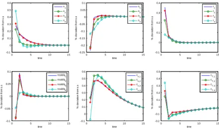
We now focus the attention on the possible e¤ects of two di¤erent demand shocks: i) a positive shock in preferences for housing in the debtor country, H (so as to proxy the demand shock for houses in countries characterized by great amount of net external liabilities); a positive shock on preferences for tradables in country F (so as to proxy a generalized in‡ation boom). Indeed, as suggested by Iacoviello and Neri (2008), demand shocks have played a major role in explaining the cyclical volatility of houses and prices in recent years.
4.2.1. Demand shock in the housing sector
Suppose now that country H is a¤ected by a positive shock in consumers’pref-erences such that its inhabitants desire to buy more houses. For simplicity, we
suppose that the shock has a log-normal distribution such that51:
pn;t = npn;t 1+ ut
ut (iid)
where we let n= 0:85, following the calibration of Iacoviello (2005).
We see that in response to an increase in households’appetite for real properties, the …nancial accelerator is at work. The increase in the stock of real assets – and
thus, in housing relative prices – entails a better access to credit.52 Since agents
4 8Caroll and Samwick (1997) estimate discount factors to be in a range between 0.91 and 0.99. 4 9It is also consistent with current trends in industrial countries, see IMF (2008).
5 0See Bils and Klenow (2004) and Monacelli (2007) for some recent discussion on the frequency
of price adjustment in U.S.
5 1The utility function is thus: max E
0 Pt=0 tUt epn;tCn;t; CT ;t; Nt 5 2Indeed, the marginal value of borrowing, ; decreases.
in country H are impatient, they use all their collateral to obtain credit. In turn, this allows them to consume tradables and to further increase their stock of houses: external debt increases on impact and continues to gradually accumulate before the shock is absorbed. The accumulation of collateral is accommodated by a gradual decrease in the user cost of durables. By inspecting equation (18) – see also the Appendix –, one can see that the user cost of durables is a positive function of
both the interest rate and the relative price of durables.53 Both relative prices and
interest rates jump on impact and decrease gradually.
Given the expansion of debt, interest rates increase; notice in particular that in absence of nominal rigidities, the interest rate and the level of in‡ation are determined by the Taylor rule together with the modi…ed Euler equations of the borrower. Indeed, the central bank reacts to the expansionary e¤ects of the shocks by tightening interest rates.
Notice in particular that in our two-country world, developments a¤ecting hous-ing prices are transmitted internationally through terms of trades. The transmission channel is evident in absence of prices rigidities. If prices are ‡exible, real marginal costs need to be constant in each period. In our case, given an identical mark-up
for all sectors54 and mobile labor across sectors, it always needs to hold:
1 xt UN;t UT ;tAn;t = (" 1) " = 1 Ah;t UN;t UT ;t h + (1 ) St1 i 1 1 (52) implying that the increase in housing relative prices entails an improvement in
terms of trade. Eventually this will transmit the e¤ect of the shock to country F .55
Borrowers enjoy thus a positive income e¤ect. As you can see in (52), the decrease in S enhances the consumption of tradables. Moreover, the decrease in the relative price of foreign goods prompts borrowers to substitute Home with Foreign tradables consumption; this switching e¤ect entails a trade de…cit. The trade de…cit together with a (quantitatively small) increase in interest payments triggers the insurgence of a current account de…cit.
Thanks to the income e¤ect, aggregate labor supply does not increase on impact in country H (as expected, it does increase in country F ): indeed, the positive income e¤ect deriving from the improvement in terms of trade o¤sets the increase in aggregate consumption in H. Aggregate labor gradually increases as soon as terms of trade start deteriorating, before of the absorption of the shock.
Notice in particular that we have assumed that debt contracts are stipulated in nominal terms. In a closed economy framework, Iacoviello (2005) and Monacelli (2007) show that an increase in in‡ation implies a shift of resources in favour of the borrower. In our framework, the impact of shocks on in‡ation is a¤ected by terms of trade. In turn, the impact of terms of trade on the in‡ation index of tradables is generally not uniquely signed. Indeed, terms of trade a¤ect both the
Home-produced tradables in‡ation56 and the CPI index of in‡ation, according to
de…nition (1) and (20).57 Clearly, if CPI in‡ation rises, real interest payments
decrease.
5 3For a focus on the role of , see the above discussion: See also Monacelli (2008) with a similar
(but not identical) collateral constraint.
5 4Clearly, qualitative results would hold also with di¤erent mark-up.
5 5For a more detailed discussion on the trasmission of shocks between countries, see the following
section.
5 6Marginal costs in the Home tradable sector are a positive functon of terms of trade 5 7In response to the preference shock for housing
T < h, if prices are ‡exible: However, if
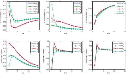
The fall in terms of trade plays a double role in response to the shock: on the one hand, by making Foreign consumption cheaper, it accommodates borrowers’ impatience and willingness to increase current consumption. On the other hand, it enhances lenders’ accumulation of Foreign currency assets and thus, their fu-ture investment incomes – we remind the readers that lenders are consumption smoother. Notice indeed that the amount of Foreign external assets is a negative function of terms of trade, according to (21). This is due to a revaluation e¤ect of lenders’ assets. Notice that the structure of our two-country world is charac-terized by the fact that borrowers do not lend; therefore, borrowers’ net external liabilities coincide with their gross external liabilities. In turn, given that borrow-ers’ debt is denominated in Home currency, assets revaluation e¤ects associated
to exchange rate swings are ruled out.58 Conversely, given that lenders are not
indebted and their holdings of gross and net external assets coincide, their wealth is subject to revaluation e¤ects associated to exchange-rate ‡uctuations. As you can see in Figure 2, the fall in S has a positive impact on Foreign external assets, which is associated to the initial appreciation of the nominal exchange rate. Notice also that given home bias, the improvement of terms of trade is associated to a real appreciation in the …rst period; indeed, the (nominal and real) exchange rate undershoots on impact so as to depreciate during the adjustment process. At the end of the adjustment, the nominal exchange rate is eventually more depreciated than its pre-shock value.
The current account de…cit is eventually absorbed as a consequence of the grad-ual decrease in borrowers’tradable consumption on the one hand; and the decrease in borrowers’ability to access to credit, on the other.
To conclude, the above results show that in response to a preference shock for durables, the increase in house relative prices is transmitted internationally through an improvement in terms of trade: house prices and terms of trade move in opposite directions. Borrowers experience a current account de…cit; the exchange rate appreciates on impact and depreciates throughout the adjustment. Notice interestingly that these trends are consistent with US data on current account, house prices and exchange rates during the last years. Around 2005, the US have experienced a steeper increase in house prices, a temporary undershooting of the
exchange rate and a deterioration of the current account (see Figure 1a, 1b).59 Our
results are consistent with Iacoviello and Neri (2008). According to their empirical analysis, during the 2000-2005 period, housing preference shocks played a major role in explaining the boom in housing investments and prices in US.
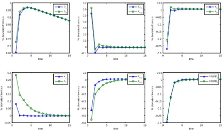
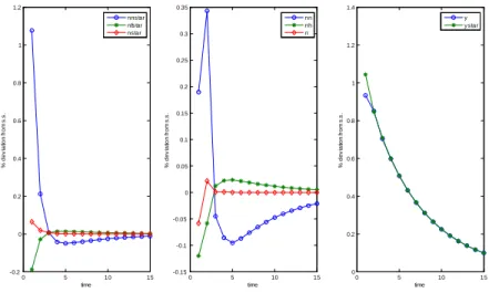
Nominal rigidities In Figure 3, we show the e¤ect of the above shock in
pres-ence of di¤erent types of price rigidities. We compare the dynamics of variables when tradables have a 4 quarter frequency in price adjustment (case 1 in Figure 3), with the case of price ‡exibility (case 2) and the case where only house prices have a 4 quarter frequency in price adjustment (case 3).
Figure 3 shows that the scenario characterized by price ‡exibility is intermediate between the other two. The main e¤ect of price rigidities lies in their impact on the relative price durables-tradables.
5 8In presence of Home-denominated debt and foreign denominated assets, revaluation e¤ects on
foreign assets can have a signi…cant impact on the dynamics of external debt. For some discussion, see, among many others, Gourinchas and Rey (2007), Iliopulos and Miller (2007), Obstfeld and Rogo¤ (2004), IMF (2005a).
If tradables are sticky, the relative price of durables jumps higher than when prices are ‡exible because the price of tradables does not immediately adjust to the expansionary e¤ect of the shock. Notice that since the prices of durables are here kept ‡exible, it still needs to hold: x1
t
UN;t
UT ;tAn;t =
(" 1)
" : In the tradable-goods sector
in‡ation is now pinned down by the New Keynesian Phillips curve, (30). Therefore, terms of trade and the relative price of durables are no more directly linked; still, they continue to move inversely. Following the jump in x, terms of trade improve but in a smaller extent (indeed, the price of Home produced goods increase more slowly).
Following the stronger jump in relative prices, the user cost of durables jumps higher; thus, agents a¤ord a smaller amount of real properties. Having said that, the increase in the value of houses allows them to continue borrowing so as to increase consumption; there is thus a switching e¤ect in favour of tradable consumption. Notice however that the dynamics of the current account are not a¤ected by price rigidities; indeed, the switching e¤ect in favour of tradable consumption is o¤set by the smaller extent of the switching e¤ect in favour of Foreign tradables (due to the weaker improvement of terms of trade). Finally the e¤ects of price rigidities are not
quantitatively relevant for the dynamics of the real exchange rate60. As in Ferrero
et al. (2008), the behavior of real-international variables do not di¤er signi…cantly from the ‡exible-case scenario: they depend mainly on real factors.
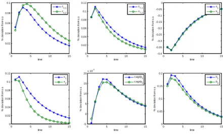
Monetary policy We now focus on the role of monetary policy. We choose to
assume the perspective of the Home central bank; we aim at investigating the e¤ects of di¤erent targets on the dynamics of our collateral-constrained open economy. Given the structure of our two-country two-sector economy, policy makers in each country can choose alternative targets: tradable goods in‡ation, Home-produced goods in‡ation and durable-goods in‡ation.
We consider the following alternative simple monetary rules: Rt R = h;t h 1;h ; 1;h! 1 (53) Rt R = T ;t T 1;h n;t n 2;h (54) Rt R = T ;t T 1;h ; 1;h! 1 (55)
together with the benchmark rule, (47). According to rule (53) (i.e., scenario 2 in the simulations of Figure 4), the monetary authority stabilizes in‡ation of Home
produced goods only (i.e., 2;h = 0 and 1;h is large). According to rule (54),
scenario 3, the central bank targets both CPI-in‡ation and in‡ation in the housing sector. Notice however that this speci…cation implies that the monetary authority directly targets also the in‡ation of imported goods; in this way, s/he directly
responds to shocks that may be imported from abroad.61 Finally, when the central
bank follows rule (55), scenario 4, s/he responds to tradable (CPI) in‡ation but disregards the trends of house prices.
6 0However, price rigidities in the tradable sector introduce larger swings in the nominal exchange
rate.
6 1One could think of commodities such as oil. For instance, by targeting core in‡ation, the Fed