HAL Id: hal-02377108
https://hal.inria.fr/hal-02377108v3
Submitted on 15 Sep 2020
HAL is a multi-disciplinary open access
archive for the deposit and dissemination of sci-entific research documents, whether they are pub-lished or not. The documents may come from teaching and research institutions in France or abroad, or from public or private research centers.
L’archive ouverte pluridisciplinaire HAL, est destinée au dépôt et à la diffusion de documents scientifiques de niveau recherche, publiés ou non, émanant des établissements d’enseignement et de recherche français ou étrangers, des laboratoires publics ou privés.
A forward-backward probabilistic algorithm for the
incompressible Navier-Stokes equations
Antoine Lejay, Hernán Mardones González
To cite this version:
Antoine Lejay, Hernán Mardones González. A forward-backward probabilistic algorithm for the in-compressible Navier-Stokes equations. Journal of Computational Physics, Elsevier, 2020, 420 (109689), �10.1016/j.jcp.2020.109689�. �hal-02377108v3�
A forward-backward probabilistic algorithm for the
incompressible Navier-Stokes equations
Antoine Lejay
*Hernán Mardones González
†May 21, 2020
Abstract
A novel probabilistic scheme for solving the incompressible Navier-Stokes equations is studied, in which we approximate a generalized nonlinear Feyman-Kac formula. The veloc-ity field is interpreted as the mean value of a stochastic process ruled by Forward-Backward Stochastic Differential Equations (FBSDEs) driven by Brownian motion. Following an ap-proach by Delbaen, Qiu and Tang introduced in 2015, the pressure term is obtained from the velocity by solving a Poisson problem as computing the expectation of an integral functional associated to an extra BSDE. The FBSDEs components are numerically solved by using a forward-backward algorithm based on Euler type schemes for the local time integration and the quantization of the increments of Brownian motion following the al-gorithm proposed by Delarue and Menozzi in 2006. Numerical results are reported on spatially periodic analytic solutions of the Navier-Stokes equations for incompressible flu-ids. We illustrate the proposed algorithm on a two dimensional Taylor-Green vortex and three dimensional Beltrami flows.
Keywords: Navier-Stokes equations ∙ Brownian motion ∙ Feynman-Kac formula ∙ forward-backward stochastic differential equations ∙ incompressible fluids ∙ numerical solution
1
Introduction
The Navier-Stokes equations system allows us to model the movement of fluids. It was intro-duced by C.-L. Navier in 1822 [52] and G. G. Stokes in 1849 [62] by incorporating a pressure term and the fluid viscosity to the Euler equations due to L.‘Euler in 1757 [27]. Nowadays, technological and scientific computing developments provide a suitable way for the simulation of mathematical models, and in turn research and analysis of efficient numerical methodologies to approximate exact solutions. With this in mind, we study the numerical simulation of the Navier-Stokes equations for incompressible fluids in R𝑑 (for space dimension 𝑑 ∈ {2, 3})
{︃
𝜕𝑢
𝜕𝑡 + (𝑢 · ∇) 𝑢 = 𝜈△𝑢 − ∇𝑝 + 𝑓 ; 0 < 𝑡 ≤ 𝑇,
∇ · 𝑢 = 0, 𝑢 (0) = 𝑔, (1)
where 𝑇 > 0 is a fixed time, 𝜈 > 0 is the kinematic viscosity, 𝑓 is the external force field and 𝑔 is a given initial divergence-free vector field. The system of equations (1) describes the motion of an incompressible fluid by means of unknown fields of velocity 𝑢 (𝑡, 𝑥) ∈ R𝑑 and pressure
*Université de Lorraine, CNRS, Inria, IECL, F-54000 Nancy, France; [email protected] †Universidad de La Serena, Facultad de Ciencias, Departamento de Matemáticas, La Serena, Chile; hmardo@
𝑝 (𝑡, 𝑥) ∈ R defined for each time 𝑡 ∈ [0, 𝑇 ] and position 𝑥 ∈ R𝑑. It involves a nonlinear convective term (𝑢 · ∇) 𝑢, a diffusion term 𝜈△𝑢 and the incompressibility condition ∇ · 𝑢 = 0. Although being introduced in the nineteenth century, there are still open problems concerning the Navier-Stokes equations. Nonetheless it is usual to find works that deal with the fluid dynamics using the Navier-Stokes model (ocean modelling, atmosphere of Earth, gas dynamics, dynamic of storms, etc.) [28, 31, 9, 64]. There exists a huge literature on computational fluid dynamics, and probabilistic numerical methods for nonlinear models have gained attention during the last decades.
The Itô stochastic differential equations (SDEs) introduced during the 1940s by K. Itô’s seminal works [35, 36] are connected with partial differential equations (PDEs) by means of the celebrated Feynman-Kac formula due to R. Feynman [29] and M. Kac [38]. More recently, the theory of backward stochastic differential equations (BSDEs), initiated by É. Pardoux and S. Peng in [58], permits to obtain probabilistic representations for the solutions of a broad class of PDEs by means of systems of forward-backward SDEs (FBSDEs) through a nonlin-ear Feynman-Kac formula. Hence, the numerical solution of FBSDEs provides a stochastic algorithm to approximate solutions of nonlinear PDEs. Among the theory of SDEs, FBSDEs associated to the unsteady Navier-Stokes equations is a novel approach.
Let us assume that the solution 𝑢 of (1) is known on a time interval [0, 𝑇 ], which means that the pressure term 𝑝 is also known (the force field 𝑓 is considered as given). We define by 𝑋 the 𝑑-dimensional diffusion process associated to the differential operator 𝑢 → (𝑢 · ∇) 𝑢 + 𝜈△𝑢. With 𝑌𝑠:= −𝑢 (𝑇 − 𝑠, 𝑋𝑠) and 𝑍𝑠:= −𝐷𝑢 (𝑇 − 𝑠, 𝑋𝑠), the process (𝑋, 𝑌, 𝑍) is solution to the
FBSDEs {︃ 𝑋𝑠 = 𝑥 + ∫︀𝑠 𝑡 𝑌𝑟d𝑟 + ∫︀𝑠 𝑡 √ 2𝜈 d𝑊𝑟, 𝑌𝑠= −𝑔 (𝑋𝑇) + ∫︀𝑇 𝑠 [∇𝑝 (𝑇 − 𝑟, 𝑋𝑟) − 𝑓 (𝑇 − 𝑟, 𝑋𝑟)] d𝑟 − ∫︀𝑇 𝑠 √ 2𝜈𝑍𝑟d𝑊𝑟, (2)
where 𝑊𝑠 is a 𝑑-dimensional standard Brownian motion. The numerical solution of the
in-compressible Navier-Stokes equations (1) involves various difficulties due to the presence of a nonlinear term, the incompressibility condition as well as the computation of the pressure term. The simplified model obtained by removing the pressure term from the FBSDEs (2) is associated to the Burgers equation [8], which remains a nonlinear equation due to the term (𝑢 · ∇) 𝑢. Under appropriate conditions, the pressure term 𝑝 is given by solving a Poisson problem −△𝑝 = 𝒫(𝑢) for a given functional of the solution.
Recently F. Delbaen, J. Qiu and S. Tang introduced in [26] a new class of coupled FBSDEs associated to the incompressible Navier-Stokes equations. Since their probabilistic approach involves an extra BSDE defined on an infinite time interval for the stochastic representation of the pressure term, Delbaen et al. deduced an approximated solution to the velocity field by truncating the infinite interval of the associated FBSDEs system. Hence they proposed a numerical simulation algorithm, that follows a methodology of F. Delarue and S. Menozzi [24, 25] for FBSDEs, to simulate the incompressible Navier-Stokes equations in the whole Cartesian space.
Specialized literature on probabilistic representations to the solution of PDEs is presented through Feynman-Kac formulae or well by means of branching processes. In general, the deter-ministic solutions of particular equations are obtained through the expectation of functionals of stochastic processes. During the last years some probabilistic approaches have been proposed to deal with the Navier-Stokes equations. The random vortex methods study the incompressible Navier-Stokes system in vorticity form [15, 16, 47]. Branching processes and stochastic cas-cades present another way of interpretation [40, 4, 5, 53, 67]. The stochastic Lagrangian paths provide additional representations [17, 37, 68]. Moreover, stochastic particle systems arise from the McKean-Vlasov equations in both two and three dimensional contexts [63, 33, 32]. Recently
the systems of FBSDEs appear as a novel approach [22, 26]. The problem of relating boundary conditions on probabilistic representations presents additional challenges [6, 18, 50, 51].
The main motivation of this paper is to develop a suitable numerical framework formulated on the new probabilistic representation of Delbaen et al for solving the incompressible Navier-Stokes equation (1) in two and three spatial dimensions. The main point is to test if such a method is practically feasible, while Monte Carlo methods are in general difficult to implement for such non-linear equations. Monte Carlo methods however offer the advantage of being simple to interpret and to set-up. By considering the numerical solution associated to the system of FBSDEs and their approximation by mean values, we consider a backward regression based on the Euler-Maruyama scheme and the quantization method. The pressure gradient is recovered from the expected value of an integral functional of Brownian motion. To do this, we use the Riemann sum estimation and the quantization of the Brownian increments.
Finally, we test the performance of the novel stochastic algorithm to the simulation of spatially-periodic analytic solutions in the unsteady regime. In our simulations, the magnitude of Reynolds number range from 1 to 200. Our numerical tests show that the proposed scheme is practically implementable. However, it suffers from long run-times which motivate the de-velopment of ad hoc variance reduction schemes. This article is only a preliminary step to the development of a Monte Carlo method for solving the incompressible Navier-Stokes equation.
Outline
Section 2 details the link between FBSDEs driven by Brownian motion and deterministic PDEs through the nonlinear Feynman-Kac formula. The incompressible Navier-Stokes equations are associated to the novel FBSDEs system. Section 3 presents the numerical methodology for solving FBSDEs. We detail the approximation of mean values and the numerical treatment of integral functionals of Brownian motion. Section 4 illustrates the forward-backward prob-abilistic algorithm by solving a two-dimensional Taylor-Green vortex and three-dimensional Beltrami flows as numerical examples. Finally Section 5 is devoted to concluding remarks.
Notations
We use the following notations and conventions:
∙ We consider a filtered complete probability space (︀Ω, ℱ, (ℱ𝑡)𝑡≥0, P)︀.
∙ For each 𝑞 ≥ 1, we set
𝐿𝑞ℱ(︀Ω; R𝑑)︀ := {︀𝜉 : Ω → R𝑑 : 𝜉 is ℱ -measurable and E ‖𝜉‖𝑞 < ∞}︀ .
∙ For each 𝑚, 𝑛 ∈ Z+and 𝐴 ∈ R𝑚×𝑛, we denote by 𝐴⊤ its transpose matrix while 𝐼𝑚represents
the 𝑚 × 𝑚 identity matrix. The matrix 𝐴 ∈ R𝑛×𝑛 is said to be elliptic if there exists 𝜆 > 0
such that
⟨𝑥, 𝐴𝑥⟩ ≥ 𝜆 ‖𝑥‖ ; ∀𝑥 ∈ R𝑛. The set of 𝑚 × 𝑚 real valued symmetric non-negative matrices is
S𝑚+ :={︀𝑄 ∈ R 𝑚×𝑚
: 𝑄 = 𝑄⊤ and ⟨𝑥, 𝑄𝑥⟩ ≥ 0; ∀𝑥 ∈ R𝑚}︀ . ∙ The symbol “≈” means “is numerically approximated by”.
∙ The symbol 𝒪 means the order of estimation. For example, ℎ = 𝒪 (𝛿2) means that ℎ > 0
is depending on 𝛿 > 0 and less than 𝐾𝛿2, with constant 𝐾 independent of 𝛿. From now on
𝐾 > 0 stands for constants independent on the discretization parameters. ∙ The indicator function of a set 𝐴 is 1𝐴.
∙ The space 𝐶𝑘,𝛼(︀
R𝑑, R𝑛)︀, or simply as 𝐶𝑘,𝛼, of 𝑘-continuously differentiable functions 𝜑 : R𝑑 → R𝑛 with 𝛼 Hölder continuity for each 𝑘-order partial derivatives equipped with the norm ‖𝜑‖𝐶𝑘,𝛼 := sup 𝑥∈R𝑑 ‖𝜑 (𝑥)‖ + 𝑘 ∑︁ |𝛽|=1 sup 𝑥∈R𝑑 ⃦ ⃦𝐷𝛽𝜑 (𝑥)⃦⃦+ ∑︁ |𝛽|=𝑘 sup 𝑥,𝑦∈R𝑑, 𝑥̸=𝑦 ⃦ ⃦𝐷𝛽𝜑 (𝑥) − 𝐷𝛽𝜑 (𝑦)⃦⃦ ‖𝑥 − 𝑦‖𝛼 .
The multi-index notation is considered.
∙ For 𝑇 > 0 and 𝑡 ∈ [0, 𝑇 ) we denote by 𝐶 ([𝑡, 𝑇 ] ; R𝑚×𝑛) the space of continuous functions 𝜓
with norm
‖𝜓‖𝐶([𝑡,𝑇 ];R𝑚×𝑛):= sup
𝑠∈[𝑡,𝑇 ]
‖𝜓 (𝑠)‖ .
Similarly we have the space 𝐶(︀[𝑡, 𝑇 ] ; 𝐶𝑘,𝛼)︀ of continuous functions with
‖𝜓‖𝐶([𝑡,𝑇 ];𝐶𝑘,𝛼) := sup
𝑠∈[𝑡,𝑇 ]
‖𝜓 (𝑠)‖𝐶𝑘,𝛼.
∙ Let 𝐿2
ℱ(Ω × [𝑡, 𝑇 ] ; R𝑚×𝑛) the space of predictable stochastic processes Ψ with values in R𝑚×𝑛
suth that E (︂∫︁ 𝑇 𝑡 ‖Ψ𝑠‖2𝑑𝑠 )︂1/2 < ∞. ∙ Let 𝐿2
ℱ(Ω; 𝐶 ([𝑡, 𝑇 ] ; R𝑚×𝑛)) be the set of all {ℱ𝑡}𝑡≥0-progressively measurable stochastic
pro-cesses Ψ with continuous trajectories taking values in R𝑚×𝑛 such that
E sup
𝑠∈[𝑡,𝑇 ]
‖Ψ𝑠‖2 < ∞.
∙ For 𝑚 ∈ N and 𝑞 ∈ [1, ∞) we denote by 𝐿𝑞(︀
Rℓ)︀ and 𝐻𝑚,𝑞(︀Rℓ)︀ the usual Rℓ-valued Lebesgue and Sobolev spaces on R𝑑, respectively. When ℓ = 𝑑 we just write 𝐿𝑞 and 𝐻𝑚,𝑞, or 𝐻𝑚 when
𝑞 = 2. ∙ The space 𝐻𝑚 𝜎 is the completion of {︀𝜑 ∈ 𝐶 ∞ 𝑐 (︀
R𝑑)︀ : div 𝜑 = 0}︀ under the norm
‖𝜑‖𝐻𝑚 𝜎 := sup 𝑥∈R𝑑 ‖𝜑 (𝑥)‖ + 𝑚 ∑︁ |𝛽|=1 sup 𝑥∈R𝑑 ⃦ ⃦𝐷𝛽𝜑 (𝑥)⃦⃦.
The space 𝐶 ([0, 𝑇 ] ; 𝐻𝜎𝑚) of continuous functions 𝜓 is equipped with ‖𝜓‖𝐶([0,𝑇 ];𝐻𝑚
𝜎 ) := sup
𝑠∈[0,𝑇 ]
‖𝜓 (𝑠)‖𝐻𝑚 𝜎 .
2
Forward-backward stochastic differential equations
Diffusion processes are linked to PDEs through the celebrated Feynman-Kac formula. The theory of Itô SDEs together Backward SDEs constitute systems of FBSDEs that are connected with deterministic nonlinear PDEs through a nonlinear Feynman-Kac formula, generalizing the classical Feynman-Kac formula (see e.g. [1, 42, 10]).
Let 𝑇 > 0, 𝑡 ∈ [0, 𝑇 ) and 𝑥 ∈ R𝑑 be fixed. Consider the FBSDEs on [𝑡, 𝑇 ] of the form
{︃ 𝑋𝑠 = 𝑥 + ∫︀𝑠 𝑡 𝑏 (𝑟, 𝑋𝑟, 𝑌𝑟, 𝑍𝑟) d𝑟 + ∫︀𝑠 𝑡 𝜎 (𝑟, 𝑋𝑟, 𝑌𝑟) d𝑊𝑟, 𝑌𝑠 = 𝑔 (𝑋𝑇) + ∫︀𝑇 𝑠 ℎ (𝑟, 𝑋𝑟, 𝑌𝑟, 𝑍𝑟) d𝑟 − ∫︀𝑇 𝑠 𝑍𝑟d𝑊𝑟, (3)
where 𝑏 : [0, 𝑇 ] × R𝑑 × R𝑛 × R𝑛×𝑚 → R𝑑 , 𝜎 : [0, 𝑇 ] × R𝑑 × R𝑛 → R𝑑×𝑚 , 𝑔 : R𝑑 → R𝑛,
ℎ : [0, 𝑇 ] × R𝑑× R𝑛× R𝑛×𝑚 → R𝑛 are given and 𝑊 = (𝑊1, . . . , 𝑊𝑚)⊤ is a 𝑚-dimensional
Wiener process defined on(︀Ω, ℱ, (ℱ𝑡)𝑡≥0, P)︀. Here, ℱ𝑡≥0 is the natural filtration of the Wiener
process 𝑊 augmented with P-null sets. An adapted solution of the FBSDEs (3) is defined by a triple of processes
(𝑋, 𝑌, 𝑍) ∈ 𝐿2ℱ(︀Ω; 𝐶 (︀[𝑡, 𝑇 ] ; R𝑑)︀)︀ × 𝐿2ℱ(Ω; 𝐶 ([𝑡, 𝑇 ] ; R𝑛)) × 𝐿2ℱ(︀Ω × [𝑡, 𝑇 ] ; R𝑛×𝑚)︀ that satisfies (3) P-almost surely. The BSDE in the system (3) depends on the diffusion process 𝑋 that solves the forward SDE. When the coefficients of the diffusion process 𝑋 do not depend on 𝑌 nor 𝑍, (3) is referred as a decoupled FBSDEs. Otherwise we have a coupled FBSDEs. From now on, we denote by (𝑋𝑡,𝑥, 𝑌𝑡,𝑥, 𝑍𝑡,𝑥) to recall the dependence on the parameters (𝑡, 𝑥) ∈
[0, 𝑇 ) × R𝑑. We refer for example to [57, 23] for the classic theory of FBSDEs.
2.1
Nonlinear Feynman-Kac formula
As in the spirit of the Feynman-Kac formula, it is possible to obtain a probabilistic repre-sentation for the solution 𝑢 = (𝑢1, . . . , 𝑢𝑛)
⊤
: [0, 𝑇 ] × R𝑑 → R𝑛 of the backward quasilinear
PDE {︃ 𝜕𝑢 𝜕𝑡 (𝑡, 𝑥) + ℒ (𝑡, 𝑥, 𝑢 (𝑡, 𝑥)) + ℎ (𝑡, 𝑥, 𝑢 (𝑡, 𝑥) , 𝐷𝑢 (𝑡, 𝑥) 𝜎 (𝑡, 𝑥, 𝑢 (𝑡, 𝑥))) = 0 ; ∀ (𝑡, 𝑥) ∈ [0, 𝑇 ) × R 𝑑, 𝑢 (𝑇, 𝑥) = 𝑔 (𝑥) ; ∀𝑥 ∈ R𝑑, (4) where 𝐷𝑢 =(︁𝜕𝑢𝑖 𝜕𝑥𝑗 )︁
𝑖,𝑗, with 𝑖 ∈ {1, . . . , 𝑛} , 𝑗 ∈ {1, . . . , 𝑑}, and Itô diffusion generator
ℒ (𝑡, 𝑥, 𝑢) := ⎛ ⎜ ⎝ 𝐿 (𝑡, 𝑥, 𝑢, 𝐷𝑢1, 𝐷2𝑢1) .. . 𝐿 (𝑡, 𝑥, 𝑢, 𝐷𝑢𝑛, 𝐷2𝑢𝑛) ⎞ ⎟ ⎠, with 𝐷𝑢𝑘 = (︁ 𝜕𝑢𝑘 𝜕𝑥1, . . . , 𝜕𝑢𝑘 𝜕𝑥𝑑 )︁⊤ , 𝐷2𝑢 𝑘 = (︁ 𝜕2𝑢 𝑘 𝜕𝑥𝑖𝜕𝑥𝑗 )︁ 𝑖,𝑗 and 𝐿 (𝑡, 𝑥, 𝑢, 𝑝, 𝑄) := 1 2tr{︀𝜎𝜎 ⊤(𝑡, 𝑥, 𝑢) 𝑄}︀ + ⟨𝑏 (𝑡, 𝑥, 𝑢, 𝐷𝑢 (𝑡, 𝑥) 𝜎 (𝑡, 𝑥, 𝑢)) , 𝑝⟩, for 𝑝 ∈ R𝑑 and 𝑄 ∈ S𝑑
+. More precisely, if the FBSDEs (3) admits unique adapted solutions
(𝑋𝑡,𝑥, 𝑌𝑡,𝑥, 𝑍𝑡,𝑥) on each subintervals [𝑡, 𝑇 ] ⊆ [0, 𝑇 ] then
𝑌𝑠𝑡,𝑥 = 𝑢(︀𝑠, 𝑋𝑠𝑡,𝑥)︀ , 𝑍𝑠𝑡,𝑥 = 𝐷𝑢(︀𝑠, 𝑋𝑠𝑡,𝑥)︀ 𝜎 (︀𝑠, 𝑋𝑠𝑡,𝑥, 𝑌𝑠𝑡,𝑥)︀ ; ∀ (𝑠, 𝑥) ∈ [𝑡, 𝑇 ] × R𝑑.
Therefore, the function 𝑢 (𝑡, 𝑥) := 𝑌𝑡𝑡,𝑥 is a viscosity solution to the associated PDE (4) (see [21]). The relation 𝑢 (𝑡, 𝑥) = 𝑌𝑡𝑡,𝑥 is called the nonlinear Feynman-Kac formula.
From now on, we assume that 𝜎𝜎⊤is uniformly elliptic i.e. the diffusion matrices 𝜎𝜎⊤(𝑡, 𝑥, 𝑦) are elliptic for all (𝑡, 𝑥, 𝑦) ∈ [0, 𝑇 ]×R𝑑×R𝑛. In particular, when ℎ (𝑡, 𝑥, 𝑦, 𝑧) = 𝑐 (𝑡, 𝑥) 𝑦 +𝑓 (𝑡, 𝑥)
and 𝑛 = 1, the BSDE in (3) has explicit solution
𝑌𝑠𝑡,𝑥 = exp {︂∫︁ 𝑇 𝑠 𝑐(︀𝑟, 𝑋𝑡,𝑥 𝑟 )︀ d𝑟 }︂ 𝑔(︀𝑋𝑡,𝑥 𝑇 )︀ + ∫︁ 𝑇 𝑠 exp {︂∫︁ 𝑟 𝑠 𝑐(︀𝜃, 𝑋𝑡,𝑥 𝜃 )︀ 𝑑𝜃 }︂ 𝑓(︀𝑟, 𝑋𝑡,𝑥 𝑟 )︀ d𝑟 − ∫︁ 𝑇 𝑠 exp {︂∫︁ 𝑟 𝑠 𝑐(︀𝜃, 𝑋𝑡,𝑥 𝜃 )︀ 𝑑𝜃 }︂ 𝑍𝑟𝑡,𝑥d𝑊𝑟.
In this case, the solution 𝑢 : [0, 𝑇 ] × R𝑑 → R of the concerned PDE (4) can be expressed as 𝑢 (𝑡, 𝑥) = 𝑌𝑡𝑡,𝑥 = E(︀𝑌𝑡𝑡,𝑥|𝑋𝑡= 𝑥)︀, that is 𝑢 (𝑡, 𝑥) = E [︂ exp {︂∫︁ 𝑇 𝑡 𝑐(︀𝑟, 𝑋𝑟𝑡,𝑥)︀ d𝑟 }︂ 𝑔(︀𝑋𝑇𝑡,𝑥)︀ + ∫︁ 𝑇 𝑡 exp {︂∫︁ 𝑠 𝑡 𝑐(︀𝑟, 𝑋𝑟𝑡,𝑥)︀ d𝑟 }︂ 𝑓(︀𝑠, 𝑋𝑠𝑡,𝑥)︀ d𝑠 ]︂ ,
which corresponds to the well-known Feynman-Kac formula (see e.g. [45, 56, 59]).
In the case of the 𝑑-dimensional viscous Burgers equation (from now on, we use 𝜈/2 as viscosity instead of 𝜈 for the sake of simplicity)
{︃ 𝜕𝑢 𝜕𝑡 + (𝑢 · ∇) 𝑢 + 𝜈 2△𝑢 + 𝑓 = 0 ; 0 ≤ 𝑡 < 𝑇, 𝑢 (𝑇 ) = 𝑔, (5) where 𝑓 : [0, 𝑇 ] × R𝑑→ R𝑑
, 𝑔 : R𝑑→ R𝑑 and 𝜈 > 0, we can associate the coupled FBSDEs
{︃
𝑋𝑠𝑡,𝑥 = 𝑥 +∫︀𝑡𝑠𝑌𝑟𝑡,𝑥d𝑟 +∫︀𝑡𝑠√𝜈 d𝑊𝑟,
𝑌𝑠𝑡,𝑥 = 𝑔(︀𝑋𝑇𝑡,𝑥)︀ + ∫︀𝑠𝑇 𝑓 (𝑟, 𝑋𝑟𝑡,𝑥) d𝑟 −∫︀𝑠𝑇√𝜈𝑍𝑟𝑡,𝑥d𝑊𝑟.
(6)
Then, 𝑌𝑡,𝑥
𝑠 = 𝑢 (𝑠, 𝑋𝑠𝑡,𝑥) and 𝑍𝑠𝑡,𝑥 = 𝐷𝑢 (𝑠, 𝑋𝑠𝑡,𝑥) for all (𝑠, 𝑥) ∈ [𝑡, 𝑇 ] × R𝑑 (see e.g. Theorem
4.1 in [43]). Alternatively, (5) admits the decoupled FBSDEs representation {︃𝑋𝑡,𝑥 𝑠 = 𝑥 + ∫︀𝑠 𝑡 √ 𝜈 d𝑊𝑟, 𝑌𝑡,𝑥 𝑠 = 𝑔(︀𝑋 𝑡,𝑥 𝑇 )︀ + ∫︀ 𝑇 𝑠 [︁ 𝑓 (𝑟, 𝑋𝑡,𝑥 𝑟 ) + 1 √ 𝜈𝑍 𝑡,𝑥 𝑟 𝑌𝑟𝑡,𝑥 ]︁ d𝑟 −∫︀𝑇 𝑠 √ 𝜈𝑍𝑡,𝑥 𝑟 d𝑊𝑟. (7)
In the coupled FBSDEs (6) the process 𝑍𝑡,𝑥 can be removed by considering the conditional
expectation E(︀· | 𝑋𝑡𝑡,𝑥 = 𝑥)︀, so that it is not necessary to compute it in order to estimate 𝑌𝑡,𝑥.
This is an advantage compared to the decoupled representation (7) if we only are interested in the estimation of the process 𝑌𝑡,𝑥
𝑠 without information about 𝑍𝑠𝑡,𝑥.
2.2
The Incompressible Navier-Stokes equations
From now on, by abuse of notation, we consider the backward Navier-Stokes equations for incompressible fluids in R𝑑, for 𝑑 ∈ {2, 3},
{︃𝜕𝑢
𝜕𝑡 + (𝑢 · ∇) 𝑢 + 𝜈
2△𝑢 + ∇𝑝 + 𝑓 = 0 ; 0 ≤ 𝑡 < 𝑇,
∇ · 𝑢 = 0, 𝑢 (𝑇 ) = 𝑔, (8)
which is equivalent to the classical formulation (1) by a time-reversing transformation (still with 𝜈/2 as viscosity). The Burgers equation (5) can be seen as a simplified version of the incompressible Navier-Stokes equations (8). Under regularity assumptions and supposing a divergence-free external force field 𝑓 , an approach to incorporate both the pressure term ∇𝑝 and the incompressibility condition ∇ · 𝑢 = 0 into the Burgers equation (5) is to consider the Poisson problem
−△𝑝 = div div (𝑢 ⊗ 𝑢) ,
where div :=∇· represents the divergence operator and ⊗ the tensor product (see e.g. [12, 44]). Then the incompressible Navier-Stokes equations system (8) is equivalent to
{︃ 𝜕𝑢 𝜕𝑡 + 𝜈 2△𝑢 + (𝑢 · ∇) 𝑢 + ∇ (−△) −1 div div (𝑢 ⊗ 𝑢) + 𝑓 = 0 ; 0 ≤ 𝑡 < 𝑇, 𝑢 (𝑇 ) = 𝑔. (9)
F. Delbaen et al [26] introduced a coupled FBSDEs system (FBSDS) associated to (9) through the nonlinear Feynman-Kac formula 𝑢 (𝑡, 𝑥) = 𝑌𝑡𝑡,𝑥 and the probabilistic representation ∇𝑝 = ̃︀𝑌0 where ̃︀𝑌 is itself solution to a BSDE involving a Brownian motion 𝐵 independent
from the one of the diffusion. The nonlocal operator ∇ (−△)−1div div is represented by means of the BSDE defined on the infinite time interval (0, ∞). Then, incorporating this extra BSDE to the FBSDEs (6) it is obtained a stochastic representation to the unsteady Navier-Stokes equations. More precisely, this new FBSDEs representation is
⎧ ⎪ ⎪ ⎪ ⎪ ⎪ ⎪ ⎪ ⎪ ⎪ ⎪ ⎨ ⎪ ⎪ ⎪ ⎪ ⎪ ⎪ ⎪ ⎪ ⎪ ⎪ ⎩ 𝑑𝑋𝑠𝑡,𝑥 = 𝑌𝑠𝑡,𝑥d𝑠 +√𝜈 d𝑊𝑠 ; 𝑠 ∈ [𝑡, 𝑇 ] , 𝑋𝑡𝑡,𝑥 = 𝑥, −𝑑𝑌𝑡,𝑥 𝑠 = [︁ 𝑓 (𝑠, 𝑋𝑡,𝑥 𝑠 ) + ̃︀𝑌0(𝑠, 𝑋𝑠𝑡,𝑥) ]︁ d𝑠 −√𝜈𝑍𝑡,𝑥 𝑠 d𝑊𝑠 ; 𝑠 ∈ [𝑡, 𝑇 ] , 𝑌𝑇𝑡,𝑥 = 𝑔(︀𝑋𝑇𝑡,𝑥)︀ , −𝑑 ̃︀𝑌𝑟𝑠,𝑥= 2𝑟273𝑌 𝑖 𝑠 · 𝑌𝑠𝑗(𝑠, 𝑥 + 𝐵𝑟) (︁ 𝐵𝑟− 𝐵2𝑟 3 )︁𝑖(︁ 𝐵2𝑟 3 − 𝐵 𝑟 3 )︁𝑗 𝐵𝑟 3 d𝑟 − ̃︀𝑍 𝑠,𝑥 𝑟 d𝐵𝑟 ; 𝑟 ∈ (0, ∞) , ̃︀ 𝑌𝑠,𝑥 ∞ = 0, (10) where 𝑊 and 𝐵 are two independent 𝑑-dimensional Brownian motions. Here ̃︀𝑌0(𝑠, 𝑋𝑠𝑡,𝑥) and
𝑌𝑠(𝑠, 𝑥 + 𝐵𝑟) means ̃︀𝑌𝑠,𝑋
𝑡,𝑥 𝑠
0 and 𝑌𝑠𝑠,𝑥+𝐵𝑟, respectively.
In [26], the infinite interval (0, ∞) of the probabilistic representation for the operator ∇ (−△)−1div div is restricted to [︀𝑁1, 𝑁]︀, for 𝑁 ∈ (1, ∞). Hence the solution 𝑢 of (9) on (𝑇0, 𝑇 ], with 𝑇0 ∈ [0, 𝑇 ), is approximated by 𝑢𝑁 which solves the PDE
{︃ 𝜕𝑢𝑁 𝜕𝑡 + 𝜈 2△𝑢 𝑁 +(︀𝑢𝑁 · ∇)︀ 𝑢𝑁 + Q𝑁(︀𝑢𝑁 ⊗ 𝑢𝑁)︀ + 𝑓 = 0 ; 𝑇 0 ≤ 𝑡 < 𝑇, 𝑢𝑁(𝑇 ) = 𝑔, (11)
where for 𝑁 ∈ (1, ∞) and ∀𝜑, 𝜓 ∈ 𝐻𝑚, with 𝑚 > 𝑑 2 + 1, Q𝑁(𝜑 ⊗ 𝜓) (𝑥) := E ∫︁ 𝑁 1 𝑁 27 2𝑠3𝜑 𝑖· 𝜓𝑗 (𝑥 + 𝐵𝑠) (︁ 𝐵𝑠− 𝐵2𝑠 3 )︁𝑖(︁ 𝐵2𝑠 3 − 𝐵 𝑠 3 )︁𝑗 𝐵𝑠 3 d𝑠; ∀𝑥 ∈ R 𝑑 .
Given 𝜈 > 0, 𝑔 ∈ 𝐻𝜎𝑚 and 𝑓 ∈ 𝐶 ([0, 𝑇 ] ; 𝐻𝜎𝑚−1) with sufficient regularity 𝑚 > 𝑑2 + 1, ⃦ ⃦𝑢 − 𝑢𝑁⃦⃦ 𝐶([𝑡,𝑇 ];𝐶𝑘,𝛼)≤ 𝐾 𝑁𝛼4 ; ∀𝑡 ∈ (𝑇0, 𝑇 ] , (12)
for some 𝑘 ∈ Z+, 𝛼 ∈ (0, 1) and 𝐾 > 0 independent of 𝑁 (see Theorem 6.6 in [26]). Then, the
PDE (11) is associated through the nonlinear Feynman-Kac formula 𝑢𝑁(𝑡, 𝑥) = 𝑌𝑡𝑡,𝑥 to the following FBSDS ⎧ ⎪ ⎪ ⎪ ⎪ ⎪ ⎪ ⎪ ⎨ ⎪ ⎪ ⎪ ⎪ ⎪ ⎪ ⎪ ⎩ 𝑑𝑋𝑡,𝑥 𝑠 = 𝑌𝑠(𝑠, 𝑋𝑠𝑡,𝑥) d𝑠 + √ 𝜈 d𝑊𝑠 ; 𝑠 ∈ [𝑡, 𝑇 ] , 𝑋𝑡𝑡,𝑥 = 𝑥, −𝑑𝑌𝑠(𝑠, 𝑋𝑠𝑡,𝑥) =[︀𝑓 (𝑠, 𝑋𝑠𝑡,𝑥) + Q𝑁(𝑌𝑠⊗ 𝑌𝑠) (𝑠, 𝑋𝑠𝑡,𝑥)]︀ d𝑠 − √ 𝜈𝑍𝑡,𝑥 𝑠 d𝑊𝑠 ; 𝑠 ∈ [𝑡, 𝑇 ] , 𝑌𝑇 (𝑇, 𝑥) = 𝑔 (𝑥) , Q𝑁(𝑌 𝑠⊗ 𝑌𝑠) (𝑠, 𝑥) = E ∫︀𝑁 1 𝑁 27 2𝑟3𝑌𝑠𝑖· 𝑌𝑠𝑗(𝑠, 𝑥 + 𝐵𝑟) (︁ 𝐵𝑟− 𝐵2𝑟 3 )︁𝑖(︁ 𝐵2𝑟 3 − 𝐵 𝑟 3 )︁𝑗 𝐵𝑟 3 d𝑟, (13) where 𝑊 and 𝐵 are independent 𝑑-dimensional Wiener processes and, by abuse of notation, we write 𝑌𝑠(𝑡, 𝑦) := 𝑌𝑠𝑡,𝑦. Moreover, it is worth pointing out that 𝑌𝑠𝑡,· = 𝑌𝑠,𝑋
𝑡,· 𝑠
𝑠 (see Theorem 6.4
3
Numerical methodology
In this section, we specify some probabilistic algorithms for the numerical solution of FBSDEs. The stochastic representations for the solutions of the Burgers equation and the incompressible Navier-Stokes equations follow from systems (6) and (10), respectively. In the first case, we consider the approach by F. Delarue and S. Menozzi [24, 25], and then we incorporate quan-tization as a control variate variable to reduce the variance of the Monte Carlo estimation of the expected values. Then, we study the incompressible Navier-Stokes equations. To this end, we consider the numerical algorithm introduced by F. Delbaen et al [26] and then we propose a novel probabilistic algorithm by incorporating the numerical treatment of the pressure term. The rest of the section is devoted to the probabilistic tools used in the numerical algorithms.
We begin with some preliminaries to the numerical approximation of FBSDEs. More pre-cisely, let 𝑇 > 0 be fixed and given 𝑁𝑇 ∈ Z+ consider a regular mesh of [0, 𝑇 ] with time-step
ℎ := 𝑇 /𝑁𝑇 i.e. set the temporal nodes [0, 𝑇 ] ∩Tℎ, with Tℎ:= ℎ · Z, or well
𝑡𝑘:= 𝑘 · ℎ; ∀𝑘 ∈ {0, . . . , 𝑁𝑇} ,
and the infinite Cartesian grid C𝛿:= 𝛿 · Z𝑑 of uniform spatial-step 𝛿 > 0. Moreover, let Π𝛿 be
the projection mapping on the grid C𝛿 defined by
Π𝛿(𝑥) := arg min{‖𝑥 − ¯𝑥‖ : ¯𝑥 ∈C𝛿}; ∀𝑥 ∈ R𝑑.
Observe that for 𝛼-Hölder continuous functions 𝐹 : R𝑑→ R𝑑 the projection error results
‖𝐹 (𝑥) − 𝐹 (Π𝛿(𝑥))‖ ≤ 𝐾𝛿𝛼.
From now on, we consider sufficient small discretization parameters of time ℎ > 0 and space 𝛿 > 0 such that 𝛿 < ℎ (see Subsection 3.1).
For all 𝑘 ∈ {0, . . . , 𝑁𝑇 − 1}, we denote ∆𝑊𝑘 = 𝑊𝑡𝑘+1 − 𝑊𝑡𝑘 and refer as 𝑞 (∆𝑊𝑘) =
√
ℎ 𝑞(︁Δ𝑊√𝑘
ℎ
)︁
to the optimal quantization of the underlying Gaussian variable ∆𝑊𝑘. Similarly,
𝑞 (𝑊𝑠) =
√
𝑠 𝑞(︁𝑊√𝑠
𝑠
)︁
(see Subsection 3.3 below).
3.1
Burgers equation
As a first point, since the Burgers equation representation (6) we are interested in systems of FBSDEs (3) whose drift terms 𝑏 and ℎ are independent of the diffusion coefficient 𝑍 i.e. FBSDEs of the form
∀𝑠 ∈ [𝑡, 𝑇 ] , {︃ 𝑋𝑠 = 𝑥 + ∫︀𝑠 𝑡 𝑏 (𝑟, 𝑋𝑟, 𝑌𝑟) d𝑟 + ∫︀𝑠 𝑡 𝜎 (𝑟, 𝑋𝑟, 𝑌𝑟) d𝑊𝑟, 𝑌𝑠 = 𝑔 (𝑋𝑇) + ∫︀𝑇 𝑠 ℎ (𝑟, 𝑋𝑟, 𝑌𝑟) d𝑟 − ∫︀𝑇 𝑠 𝑍𝑟d𝑊𝑟. (14)
As usual, we can remove the martingale part of the BSDE by taking the conditional expectation E (·|𝑋𝑡 = 𝑥) and so the dependence of 𝑌 on the process 𝑍. Thus we focus on the numerical
solution of the process 𝑌 and, since the nonlinear Feynman-Kac formula, the estimation of the strong solution 𝑢 of the related PDE (4) by means of a probabilistic numerical algorithm.
Usually the numerical schemes for FBSDEs involve backward regressions to compute es-timations of the processes (𝑋, 𝑌, 𝑍) (see e.g. [43, 49]). The following numerical scheme ¯𝑢 approximates the process 𝑌 involved in the FBSDEs (14).
Algorithm 3.1 (F. Delarue and S. Menozzi [24]). Define ¯
For each temporal node 𝑡𝑘 with 𝑘 ∈ {0, . . . , 𝑁𝑇 − 1} and any spatial position 𝑥 ∈ C𝛿,
compute recursively
T (𝑡𝑘, 𝑥) = 𝑏 (𝑡𝑘+1, 𝑥, ¯𝑢 (𝑡𝑘+1, 𝑥)) · ℎ + 𝜎 (𝑡𝑘+1, 𝑥, ¯𝑢 (𝑡𝑘+1, 𝑥)) 𝑞 (∆𝑊𝑘) ,
¯
𝑢 (𝑡𝑘, 𝑥) = E [¯𝑢 (𝑡𝑘+1, Π𝛿(𝑥 +T (𝑡𝑘, 𝑥)))] + ℎ (𝑡𝑘+1, 𝑥, ¯𝑢 (𝑡𝑘+1, 𝑥)) · ℎ.
The process T (𝑡𝑘, 𝑥) corresponds to the Euler-Maruyama scheme applied to the Itô SDE.
Its convergence is well known in a Hölder continuous setting when the quantization of ∆𝑊𝑘 is
not considered (see [48]). Quantizing the underlying Gaussian variables 𝑞 (∆𝑊𝑘) provides us
with an efficient method to deal with the expectation approximations to the terms ¯𝑢 (𝑡𝑘, 𝑥),
instead of the classical Monte Carlo procedure. By its way the projection operator Π𝛿 onto the
spatial grid incorporates an extra source of error to the order of convergence of the numerical algorithm. The spatial discretization 𝛿 > 0 must be smaller than the time step ℎ > 0 to capture the dynamics of the drift and diffusion parts ofT (𝑡𝑘, 𝑥) in the computation of Π𝛿(𝑥 +T (𝑡𝑘, 𝑥)).
Indeed, the discretization T𝑁(𝑡
𝑘, 𝑥) has drift term of order ℎ and diffusion part of order
√ ℎ. Hence the spatial mesh has to be fine enough to capture the local influence of 𝑥 +T𝑁 (𝑡
𝑘, 𝑥) by
means of the projector Π𝛿.
All this elements are bounded to the computation of Algorithm 3.1 (see Section 4 of [24] and [25] for details and convergence).
We incorporate quantization as a control variate variable to the Monte Carlo computation of mean values (see Subsection 3.3 for details). More precisely, we introduce the following numerical scheme:
Algorithm 3.2. Define
¯
𝑢 (𝑇, 𝑥) = 𝑔 (𝑥) ; ∀𝑥 ∈ C𝛿.
For each time node 𝑘 ∈ {0, . . . , 𝑁𝑇 − 1} and any position 𝑥 ∈ C𝛿, compute
T (𝑡𝑘, 𝑥) = 𝑏 (𝑡𝑘+1, 𝑥, ¯𝑢 (𝑡𝑘+1, 𝑥)) · ℎ + 𝜎 (𝑡𝑘+1, 𝑥, ¯𝑢 (𝑡𝑘+1, 𝑥)) 𝑞 (∆𝑊𝑘) , ¯ 𝑢 (𝑡𝑘, 𝑥) = E [¯𝑢 (𝑡𝑘+1, Π𝛿(𝑥 +T (𝑡𝑘, 𝑥)))] + ℎ (𝑡𝑘+1, 𝑥, ¯𝑢 (𝑡𝑘+1, 𝑥)) · ℎ + 1 𝑀 𝑀 ∑︁ 𝑙=1 [︁ ¯ 𝑢(︀𝑡𝑘+1, Π𝛿(︀𝑥 + T(𝑙)(𝑡𝑘, 𝑥))︀)︀ − ¯𝑢 (︁ 𝑡𝑘+1, Π𝛿 (︁ 𝑥 + ̂︀T(𝑙)(𝑡𝑘, 𝑥) )︁)︁]︁ .
Here ∆𝑊𝑘(𝑙) = 𝑊𝑡(𝑙)𝑘+1 − 𝑊𝑡(𝑙)𝑘 are 𝑀 ∈ Z+ independent realizations of the Gaussian
vari-able ∆𝑊𝑘. Moreover, T(𝑙)(𝑡𝑘, 𝑥) := 𝑏 (𝑡𝑘+1, 𝑥, ¯𝑢 (𝑡𝑘+1, 𝑥)) · ℎ + 𝜎 (𝑡𝑘+1, 𝑥, ¯𝑢 (𝑡𝑘+1, 𝑥)) ∆𝑊 (𝑙) 𝑘 and ̂︀ T(𝑙)(𝑡 𝑘, 𝑥) := 𝑏 (𝑡𝑘+1, 𝑥, ¯𝑢 (𝑡𝑘+1, 𝑥)) · ℎ + 𝜎 (𝑡𝑘+1, 𝑥, ¯𝑢 (𝑡𝑘+1, 𝑥)) 𝑞 (︁ ∆𝑊𝑘(𝑙))︁.
Note that the convergence of Algorithm 3.1 involves the optimality of quantization parame-ters to the underlying Gaussian random variables. However, the quantization as control variates to the Monte Carlo method can reduce the approximation error or improve the computational effort to the calculation of the conditional expectations. In [46], Algorithm 3.2 have been tested with success to the Burgers equation in some numerical tests proposed by [24, 25].
3.2
Incompressible Navier-Stokes equations
Delbaen et al [26] propose a numerical algorithm ¯𝑢𝑁 to approximate the process 𝑌 that solves (13) and then the solution 𝑢𝑁 of (11). We present now the general algorithm which computes a
numerical approximation ¯𝑢𝑁 of the velocity field 𝑢 solution to the incompressible Navier-Stokes
Algorithm 3.3. Define
¯
𝑢𝑁(𝑇, 𝑥) = 𝑔 (𝑥) ; ∀𝑥 ∈ C𝛿.
Then for each 𝑘 ∈ {0, . . . , 𝑁𝑇 − 1} and all 𝑥 ∈ C𝛿, compute
T𝑁(𝑡𝑘, 𝑥) = ¯𝑢𝑁(𝑡𝑘+1, 𝑥) · ℎ + √ 𝜈𝑞 (∆𝑊𝑘) , Q𝑁(𝑡𝑘+1, 𝑥) = E ∫︁ 𝑁3 1 3𝑁 3 2𝑟3𝑢¯ 𝑁 𝑖 · ¯𝑢 𝑁 𝑗 (︁ 𝑡𝑘+1, Π𝛿 (︁ 𝑥 + 𝑞(︀𝐵¯𝑟)︀ + 𝑞 (︁ ̃︀ 𝐵𝑟 )︁ + 𝑞(︁𝐵̂︀𝑟 )︁)︁)︁ 𝑞𝑖(︀𝐵¯𝑟)︀ 𝑞𝑗 (︁ ̃︀ 𝐵𝑟 )︁ 𝑞(︁𝐵̂︀𝑟 )︁ d𝑟, ¯ 𝑢𝑁(𝑡𝑘, 𝑥) = E[︀ ¯𝑢𝑁(︀𝑡𝑘+1, Π𝛿(︀𝑥 + T𝑁(𝑡𝑘, 𝑥))︀)︀]︀ + (︀𝑓 (𝑡𝑘+1, 𝑥) +Q𝑁(𝑡𝑘+1, 𝑥))︀ · ℎ.
For each time 𝑡𝑘 ∈ [0, 𝑇 ], Algorithm 3.3 computes the approximation ¯𝑢𝑁(𝑡𝑘, ·) of 𝑢𝑁(𝑡𝑘, ·)
over the spatial grid, where 𝑢𝑁 solves the backward Navier-Stokes equation (9). Therefore the velocity field 𝑢 (𝑡𝑘, ·) of the incompressible Navier-Stokes equations (1) is approximated by
−¯𝑢𝑁(𝑇 − 𝑡𝑘, ·).
As is the Burgers equation context, the spatial step 𝛿 > 0 must be smaller than the time step ℎ > 0. Moreover, the probabilistic representation of the gradient pressure involves perturbations of order √𝑟 to each particle position 𝑥. It would be necessary to have spatial discretizations 𝛿 < √1
𝑁 to capture its dynamics by means of the projector Π𝛿.
Given the vector field ¯𝑢𝑁(𝑡
𝑘+1, ·) ≈ 𝑌 𝑡𝑘+1,·
𝑡𝑘+1 , the algorithm constructs the approximation
¯
𝑢𝑁(𝑡𝑘, 𝑥) of 𝑌𝑡𝑘(𝑡𝑘, 𝑥) for all 𝑥 ∈ C𝛿, with 𝑌 solving (13). This procedure involves the local
time integration ∫︁ 𝑡𝑘+1 𝑡𝑘 Q𝑁(𝑌𝑠⊗ 𝑌𝑠)(︀𝑠, 𝑋𝑠𝑡𝑘,𝑥)︀ d𝑠 ≈ E ∫︁ 𝑁 1 𝑁 27 2𝑟3𝑌 𝑖 𝑡𝑘+1 · 𝑌 𝑗 𝑡𝑘+1(𝑡𝑘+1, 𝑥 + 𝐵𝑟) (︁ 𝐵𝑟− 𝐵2𝑟 3 )︁𝑖(︁ 𝐵2𝑟 3 − 𝐵 𝑟 3 )︁𝑗 𝐵𝑟 3 d𝑟 · ℎ ≈ E ∫︁ 𝑁 1 𝑁 27 2𝑟3𝑢¯ 𝑁 𝑖 · ¯𝑢 𝑁 𝑗 (𝑡𝑘+1, 𝑥 + 𝐵𝑟) (︁ 𝐵𝑟− 𝐵2𝑟 3 )︁𝑖(︁ 𝐵2𝑟 3 − 𝐵 𝑟 3 )︁𝑗 𝐵𝑟 3 d𝑟 · ℎ = E ∫︁ 𝑁3 1 3𝑁 3 2𝑟3𝑢¯ 𝑁 𝑖 · ¯𝑢 𝑁 𝑗 (︁ 𝑡𝑘+1, 𝑥 + ¯𝐵𝑟+ ̃︀𝐵𝑟+ ̂︀𝐵𝑟)︁ ¯𝐵𝑖𝑟𝐵̃︀𝑟𝑗𝐵̂︀𝑟d𝑟 · ℎ ≈ E ∫︁ 𝑁3 1 3𝑁 3 2𝑟3𝑢¯ 𝑁 𝑖 · ¯𝑢𝑁𝑗 (︁ 𝑡𝑘+1, Π𝛿 (︁ 𝑥 + ¯𝐵𝑟+ ̃︀𝐵𝑟+ ̂︀𝐵𝑟)︁)︁ ¯𝐵𝑟𝑖𝐵̃︀𝑟𝑗𝐵̂︀𝑟d𝑟 · ℎ.
Here the increments of 𝐵 are replaced by three independent 𝑑-dimensional Brownian motions ¯
𝐵, ̃︀𝐵 and ̂︀𝐵 independent of 𝑊 . Then, involving the quantization of the underlying Gaussian random variables we obtain
∫︁ 𝑡𝑘+1
𝑡𝑘
Q𝑁(𝑌𝑠⊗ 𝑌𝑠)(︀𝑠, 𝑋𝑠𝑡𝑘,𝑥)︀ d𝑠 ≈ Q 𝑁
(𝑡𝑘+1, 𝑥) · ℎ. (15)
Computing expectations of integrals depending on paths of Brownian motions introduces an additional source of error in the numerical treatment of the pressure term. We then show how to efficiently compute 𝒬𝑁 in Algorithm 3.3 so that ¯𝑢𝑁 approximates 𝑢𝑁 given by (11) (see
Subsection 3.4).
The quantization of the underlying Gaussian variables permits us to compute mean values easily, with its estimation error depending on the dimension 𝑑 and the number of quantiza-tion points. As in the Burgers equaquantiza-tion, we can use quantizaquantiza-tion as a control variate to the estimation of the pressure term, but increasing considerably the computational effort of the algorithm especially when 𝑑 = 3. Hence, a convenient variance reduction technique needs to be considered to deal with path-dependent functionals of Brownian motion. We mention for example variance reduction techniques in [41, 39].
3.3
Estimation of conditional expectations
Suppose that 𝑈 : Ω → R𝑚 is a square integrable random variable and 𝐹 : R𝑚 → R𝑑is uniformly
𝛼-Hölder continuous with Hölder exponent 𝛼 ∈ (0, 1], such that 𝐹 (𝑈 ) ∈ 𝐿2
ℱ(︀Ω; R𝑑)︀. The usual
way to estimate expectations is by means of the Monte Carlo approximation
E [𝐹 (𝑈 )] ≈ 1 𝑀 𝑀 ∑︁ 𝑖=1 𝐹 (︀𝑈(𝑖))︀ , (16)
where 𝑈(𝑖) are 𝑀 independent realizations of the underlying random variable 𝑈 . From now
on, the averages are computed in a component-wise manner. It is well-known that the Monte Carlo method (16) converges in law to the mean E [𝐹 (𝑈 )] with estimation error depending on √︀Var 𝐹 (𝑈)/√𝑀 as 𝑀 tends to ∞.
We use the quantization method to estimate mean values. Indeed, let 𝑞 (𝑈 ) be a quantizer of 𝑈 i.e. an approximation of 𝑈 by a discrete random variable 𝑞 (𝑈 ) taking values in a finite set Γ = {𝑣1, . . . , 𝑣𝑄} ⊂ R𝑚. Suppose that 𝑞 (𝑈 ) =
∑︀𝑄
𝑖=1𝑣𝑖1𝐶𝑖(𝑈 ) where 𝐶 = {𝐶1, . . . , 𝐶𝑄} is a
partition of R𝑚 associated to Γ be means of 𝑣𝑖 ∈ 𝐶𝑖 for all 𝑖 ∈ {1, . . . , 𝑄}. Then
E [𝐹 (𝑈 )] ≈ E [𝐹 (𝑞 (𝑈 ))] =
𝑄
∑︁
𝑖=1
P (𝑈 ∈ 𝐶𝑖) · 𝐹 (𝑣𝑖) . (17)
Since 𝐹 is 𝛼-Hölder continuous, Jensen’s inequality implies that the error of estimation is bounded by
‖E [𝐹 (𝑈)] − E [𝐹 (𝑞 (𝑈))]‖ ≤ 𝐾(︀
E[︀‖𝑈 − 𝑞 (𝑈 )‖2]︀)︀
𝛼/2
, where the quantization error in the 𝐿2-norm (to the power 2) is given by
‖𝑈 − 𝑞 (𝑈 )‖22 =
𝑄
∑︁
𝑖=1
E[︀‖𝑈 − 𝑣𝑖‖21𝐶𝑖(𝑈 )]︀ .
Thus, the key point is to provide convenient sets Γ and 𝐶 such that the quadratic quantization error is optimal. An optimal quantizer is found through a stochastic gradient procedure over the positions of the points 𝑣1, . . . , 𝑣𝑄. The cells 𝐶𝑖 are then given by a Voronoï partition of the
space. Hence, for a given realization 𝑢 ∈ R𝑚 of 𝑈 , we set
𝑞(𝑢) := 𝑣𝑖 such that ‖𝑢 − 𝑣𝑖‖ ≤ ‖𝑢 − 𝑣𝑗‖ ; ∀𝑗 = 1, . . . , 𝑄, 𝑗 ̸= 𝑖.
In other words, 𝑞(𝑢) is the closest point to 𝑢 among the 𝑣𝑖’s. We refer to [34, 54, 20, 19] for
details on optimal quantization. In particular, the case of a 𝑚-dimensional Gaussian random variable 𝜉 ∼ 𝒩 (0, 𝐼𝑚) is is treated in details in [54].
A consequence from the Zador theorem [34] is that
E[‖𝜉 − 𝑞(𝜉)‖2]1/2≤ 𝐾(𝑚)𝑄−1/𝑚
where 𝐾(𝑚) is a constant which depends from the dimension 𝑚. Hence we have a non-asymptotic error bound
‖E [𝐹 (𝑈)] − E [𝐹 (𝑞 (𝑈))]‖ ≤ 𝐾 𝑄𝛼/𝑚,
depending on the dimension 𝑚 and the number 𝑄 of quantizer points. We see that quantization is better in low dimension.
Tables for optimal quantizers are provided in the web site [20], which we use for our nu-merical implementations1. Thus, given an application 𝑞 which gives the optimal quantizer for
𝜉 ∼ 𝒩 (0, 𝐼𝑚), we set
𝑞(𝜁) := 𝜇 + Σ 𝑞(︀Σ−1(𝜁 − 𝜇))︀ for 𝜁 ∼ 𝒩 (𝜇, ΣΣ𝑇).
Quantization is also a convenient tool for constructing a control variate in order to perform a variance reduction technique in Monte Carlo simulations (see e.g. [30] for an introduction to control variates). More precisely, we use
E [𝐹 (𝑈 )] ≈ E [𝐹 (𝑞 (𝑈 ))] + 1 𝑀 𝑀 ∑︁ 𝑖=1 [︀𝐹 (︀𝑈(𝑖))︀ − 𝐹 (︀𝑞 (︀𝑈(𝑖))︀)︀]︀ . (18)
The error of the estimation (18) is then √︀Var(𝐹 (𝑈) − 𝐹 (𝑞(𝑈)))/√𝑀 as 𝑀 goes to ∞. Thus, the error is reduced when 𝑞(𝑈 ) is close enough to 𝑈 . The order 𝑀−1/2𝑄−1/𝑚 is obtained for the Gaussian case. We refer to [55, 41, 19] for reduction variance techniques that use quantization. As a special case, let 𝑈1, . . . , 𝑈ℓ be ℓ independent and identically distributed square inte-grable random variables 𝑈𝑘 : Ω → R𝑚 and 𝐹 : (R𝑚)ℓ
→ R𝑑 an 𝛼-Hölder continuous function
such that 𝐹(︀𝑈1, . . . , 𝑈ℓ)︀ belongs to 𝐿2
ℱ(︀Ω; R𝑑)︀. Then, we compute E[︀𝐹 (︀𝑈1, . . . , 𝑈ℓ)︀]︀ ≈ E [︀𝐹 (︀𝑞 (︀𝑈1)︀ , . . . , 𝑞 (︀𝑈ℓ)︀)︀]︀ = 𝑄 ∑︁ 𝑖1,...,𝑖𝑙=1 P(︀𝑈1 ∈ 𝐶𝑖1)︀ × · · · × P (︀𝑈 ℓ ∈ 𝐶 𝑖𝑙)︀ 𝐹 (𝑣𝑖1, . . . , 𝑣𝑖𝑙)
because 𝑈1, . . . , 𝑈ℓ are independent. The same quantizers points are taken for each random variable.
3.4
Integrals involving paths of Brownian motions
In the FBSDS (10) the pressure term is represented by ∇𝑝(︀𝑠, 𝑋𝑡,𝑥
𝑠 )︀ =𝑌̃︀0(︀𝑠, 𝑋𝑠𝑡,𝑥)︀ .
Then the approximated solution 𝑢𝑁 is estimated by means of the stochastic process 𝑌 of the
truncated FBSDS (13) and involves its approximation Q𝑁(𝑌𝑠⊗ 𝑌𝑠) (𝑠, 𝑋𝑠𝑡,𝑥), for 𝑁 ∈ Z+. Given
the estimations ¯𝑢𝑁(𝑡
𝑘+1, 𝑥) of 𝑌𝑡𝑘+1(𝑡𝑘+1, 𝑥) for all 𝑥 ∈ C𝛿, we approximate 𝑌𝑡𝑘(𝑡𝑘, 𝑥) over the
spatial grid by locally integrating the BSDE that defines (𝑌𝑡𝑘,𝑥
𝑠 )𝑠∈[𝑡𝑘,𝑡𝑘+1]. Concerning to the
gradient of the pressure, for each 𝑘 ∈ {0, . . . , 𝑁𝑇 − 1} and 𝑥 ∈ C𝛿,
E ∫︁ 𝑡𝑘+1 𝑡𝑘 Q𝑁(𝑌𝑠⊗ 𝑌𝑠)(︀𝑠, 𝑋𝑠𝑡,𝑥)︀ 𝑑𝑠 ≈ E ∫︁ 𝑁 1 𝑁 27 2𝑟3𝑢¯ 𝑁 𝑖 · ¯𝑢 𝑁 𝑗 (𝑡𝑘+1, 𝑥 + 𝐵𝑟) (︁ 𝐵𝑟− 𝐵2𝑟 3 )︁𝑖(︁ 𝐵2𝑟 3 − 𝐵 𝑟 3 )︁𝑗 𝐵𝑟 3 d𝑟 · ℎ.
In [26], the increments of 𝐵 are replaced by three independent 𝑑-dimensional Brownian motions ¯
𝐵, ̃︀𝐵 and ̂︀𝐵 independent of 𝑊 . This procedure involves the local time integration ∫︁ 𝑡𝑘+1 𝑡𝑘 Q𝑁(𝑌𝑠⊗ 𝑌𝑠)(︀𝑠, 𝑋𝑠𝑡𝑘,𝑥)︀ 𝑑𝑠 ≈ E ∫︁ 𝑁 1 𝑁 27 2𝑟3𝑢¯ 𝑁 𝑖 · ¯𝑢 𝑁 𝑗 (𝑡𝑘+1, 𝑥 + 𝐵𝑟) (︁ 𝐵𝑟− 𝐵2𝑟 3 )︁𝑖(︁ 𝐵2𝑟 3 − 𝐵 𝑟 3 )︁𝑗 𝐵𝑟 3 d𝑟 · ℎ = E ∫︁ 𝑁3 1 3𝑁 3 2𝑟3𝑢¯ 𝑁 𝑖 · ¯𝑢𝑁𝑗 (︁ 𝑡𝑘+1, 𝑥 + ¯𝐵𝑟+ ̃︀𝐵𝑟+ ̂︀𝐵𝑟)︁ ¯𝐵𝑟𝑖𝐵̃︀𝑟𝑗𝐵̂︀𝑟d𝑟 · ℎ ≈ E ∫︁ 𝑁3 1 3𝑁 3 2𝑟3𝑢¯ 𝑁 𝑖 · ¯𝑢 𝑁 𝑗 (︁ 𝑡𝑘+1, Π𝛿 (︁ 𝑥 + ¯𝐵𝑟+ ̃︀𝐵𝑟+ ̂︀𝐵𝑟)︁)︁ ¯𝐵𝑟𝑖𝐵̃︀𝑟𝑗𝐵̂︀𝑟d𝑟 · ℎ.
1There exists several ways to consider the quantization of a vector: we could quantize each components, the
Hence denoting 𝐹 (︁𝑟, ¯𝐵𝑟, ̃︀𝐵𝑟, ̂︀𝐵𝑟 )︁ := 3 2𝑟3𝑢¯ 𝑁 𝑖 · ¯𝑢 𝑁 𝑗 (︁ 𝑡𝑘+1, Π𝛿 (︁ 𝑥 + ¯𝐵𝑟+ ̃︀𝐵𝑟+ ̂︀𝐵𝑟)︁)︁ ¯𝐵𝑟𝑖𝐵̃︀𝑟𝑗𝐵̂︀𝑟,
we aim at computing numerically the term
Q𝑁(𝑡𝑘+1, 𝑥) = E ∫︁ 𝑁3 1 3𝑁 𝐹 (︁𝑟, ¯𝐵𝑟, ̃︀𝐵𝑟, ̂︀𝐵𝑟, )︁ 𝑑𝑟 (19) for ¯𝑢𝑁 =(︀ ¯𝑢𝑁 1 , . . . , ¯𝑢𝑁𝑑 )︀⊤
and three independent 𝑑-dimensional standard Brownian motions. The size of the interval[︀3𝑁1 ,𝑁3]︀ determines the quality of the approximation in (12) so that accurate estimations are obtained for large values of 𝑁 , leading to costly Monte Carlo approximations. A first intent to compute the termQ𝑁 is to use the quantization of the underlying Gaussian
processes together with Riemann sum approximations to the integrals. Indeed, let 𝑁𝑅 ∈ Z+
and define an uniform time step 𝜏 :=(︀𝑁3 − 1
3𝑁)︀ /𝑁𝑅, with equidistant nodes
𝑠ℓ:= 1 3𝑁 + (ℓ − 1) · 𝜏 ; ∀ℓ ∈ {1, . . . , 𝑁𝑅} . Therefore, denoting by ¯ 𝜉𝑟:= ¯ 𝐵𝑟 √ 𝑟, ̃︀𝜉𝑟:= ̃︀ 𝐵𝑟 √ 𝑟, and ̂︀𝜉𝑟:= ̂︀ 𝐵𝑟 √ 𝑟, the pressure gradient term is estimated from Q𝑁 (𝑡
𝑘+1, 𝑥) ≈Q̂︀𝑁(𝑡𝑘+1, 𝑥) with ̂︀ Q𝑁(𝑡𝑘+1, 𝑥) := E 𝑁𝑅 ∑︁ ℓ=1 3 2(︀√𝑠ℓ )︀3𝑢¯ 𝑁 𝑖 · ¯𝑢 𝑁 𝑗 (︁ 𝑡𝑘+1, Π𝛿 (︁ 𝑥 +√𝑠ℓ [︁ 𝑞(︀𝜉¯𝑠ℓ)︀ + 𝑞 (︁ ̃︀ 𝜉𝑠ℓ )︁ + 𝑞(︁𝜉̂︀𝑠ℓ )︁]︁)︁)︁ × 𝑞𝑖(︀¯ 𝜉𝑠ℓ)︀ 𝑞 𝑗(︁ ̃︀ 𝜉𝑠ℓ )︁ 𝑞(︁𝜉̂︀𝑠ℓ )︁ · 𝜏. (20)
Remark 1. In case of 𝛼-Hölder continuous function 𝜑 : R𝑑→ R𝑑 we consider
𝐹(︁𝑟, ¯𝐵𝑟, ̃︀𝐵𝑟, ̂︀𝐵𝑟 )︁ := 3 2𝑟3𝜑𝑖· 𝜑𝑗 (︁ Π𝛿 (︁ 𝑥 + ¯𝐵𝑟+ ̃︀𝐵𝑟+ ̂︀𝐵𝑟)︁)︁ ¯𝐵𝑖𝑟𝐵̃︀𝑟𝑗𝐵̂︀𝑟 and take E ∫︁ 𝑁3 1 3𝑁 𝐹(︁𝑟, ¯𝐵𝑟, ̃︀𝐵𝑟, ̂︀𝐵𝑟, )︁ d𝑟 ≈ E 𝑁𝑅 ∑︁ ℓ=1 𝐹 (︁𝑠ℓ, ¯𝐵𝑠ℓ, ̃︀𝐵𝑠ℓ, ̂︀𝐵𝑠ℓ )︁ · 𝜏 ≈ E 𝑁𝑅 ∑︁ ℓ=1 𝐹 (︁𝑠ℓ, 𝑞 (︀¯ 𝐵𝑠ℓ)︀ , 𝑞 (︁ ̃︀ 𝐵𝑠ℓ )︁ , 𝑞(︁𝐵̂︀𝑠ℓ )︁)︁ · 𝜏
for all 𝑥 ∈ 𝒞𝛿, which involves simulating 𝑁𝑅× 3 × 𝑑 Gaussian random variables. The error
of estimation depends on 𝑑 ∈ {2, 3}, 𝛼 ∈ (0, 1), and the discretization parameters 𝜏 > 0 and 𝑄 ∈ Z+.
3.5
Computer implementation
The velocity field 𝑢 that solves the Navier-Stokes equations system (1) is estimated by
𝑢 (𝑡𝑘, 𝑥) ≈ −¯𝑢𝑁(𝑇 − 𝑡𝑘, 𝑥) ; ∀ (𝑡𝑘, 𝑥) ∈ [0, 𝑇 ] ∩Tℎ× [0, 2𝜋] 𝑑
To do this, we initialize ¯
𝑢𝑁(𝑇, 𝑥) = −𝑢 (0, 𝑥) ; ∀𝑥 ∈ [0, 2𝜋]𝑑∩ C𝛿.
Then for each 𝑘 from 𝑁𝑇 − 1 to 0, we compute
¯
𝑢𝑁(𝑡𝑘, 𝑥) ; ∀𝑥 ∈ [0, 2𝜋]𝑑∩ C𝛿,
from the velocity field ¯𝑢𝑁(𝑡
𝑘+1, ·) and the optimal quantizers for standard Gaussian random
variables 𝒩 (0, 𝐼𝑑). In this procedure, let ̂︀Π𝛿 be the projection mapping on the computational
grid [0, 2𝜋]𝑑∩ C𝛿 defined by ̂︀ Π𝛿(𝑥) := arg min {︁⃦ ⃦ ⃦ (︁ 𝑥 − 2𝜋 · ⌊︁ 𝑥 2𝜋 ⌋︁)︁ − ¯𝑥 ⃦ ⃦ ⃦: ¯𝑥 ∈ [0, 2𝜋] 𝑑 ∩ C𝛿 }︁ ; ∀𝑥 ∈ R𝑑.
Here ⌊·⌋ denotes the floor function. The approximation ¯𝑢𝑁 is extended by periodicity from
[0, 2𝜋]𝑑∩ C𝛿 to the complete spatial grid C𝛿.
More precisely, we present the following algorithm:
Algorithm 3.4. (1) Define the dimension 𝑑 ∈ {2, 3}, a final time 𝑇 > 0 and the viscosity parameter 𝜈 > 0. Fix the truncation parameter 𝑁 ∈ N, time-step ℎ = 𝑁𝑇𝑇;
with 𝑁𝑇 ∈ N, and spatial-step 𝛿 = 𝑁2𝜋
𝛿 > 0, with 𝑁𝛿 ∈ N. Define the initial
velocity field 𝑔 (𝑥) and the external force 𝑓 (𝑡, 𝑥) for each 𝑡 ∈ [0, 𝑇 ] ∩Tℎ and
for all 𝑥 ∈ [0, 2𝜋]𝑑∩ C𝛿. Consider 𝑄 ∈ N grid points for quantization, and
𝑁𝑅∈ N subintervals of [︀ 1 3𝑁, 𝑁 3 ]︀
with step size 𝜏 =(︀𝑁3 − 3𝑁1 )︀ /𝑁𝑅.
(2) Initialize
¯
𝑢𝑁(𝑇, 𝑥) = −𝑔 (𝑥) ; ∀𝑥 ∈ [0, 2𝜋]𝑑∩ C𝛿.
(3) For each 𝑘 from 𝑁𝑇 − 1 to 0, do for all 𝑥 ∈ [0, 2𝜋]𝑑∩ C𝛿:
̂︀ 𝑋𝑡𝑁 𝑘+1(𝑡𝑘, 𝑥) = 𝑥 + ¯𝑢 𝑁(𝑡 𝑘+1, 𝑥) · ℎ + √ 2𝜈 ·√ℎ 𝑞(︂ 𝑊𝑡𝑘+1− 𝑊𝑡𝑘 √ ℎ )︂ , ̂︀ 𝑌𝑡𝑁 𝑘 (𝑡𝑘, 𝑥) = E [︁ ¯ 𝑢𝑁(︁𝑡𝑘+1, ̂︀Π𝛿 (︁ ̂︀ 𝑋𝑡𝑁 𝑘+1(𝑡𝑘, 𝑥) )︁)︁]︁ , ̂︀ Q𝑁(𝑡𝑘+1, 𝑥) = E [︃𝑁 𝑅 ∑︁ ℓ=1 3 2(︀√𝑠ℓ )︀3𝑢¯ 𝑁 𝑖 · ¯𝑢 𝑁 𝑗 (︁ 𝑡𝑘+1, ̂︀Π𝛿 (︁ 𝑥 +√𝑠ℓ [︁ 𝑞(︀𝜉¯𝑠ℓ)︀ + 𝑞 (︁ ̃︀ 𝜉𝑠ℓ )︁ + 𝑞(︁𝜉̂︀𝑠ℓ )︁]︁)︁)︁ × 𝑞𝑖(︀¯ 𝜉𝑠ℓ)︀ 𝑞 𝑗(︁ ̃︀ 𝜉𝑠ℓ )︁ 𝑞(︁𝜉̂︀𝑠ℓ )︁ · 𝜏 ]︃ , ¯ 𝑢𝑁(𝑡𝑘, 𝑥) = ̂︀𝑌𝑡𝑁𝑘 (𝑡𝑘, 𝑥) + [︀ ̂︀ Q𝑁(𝑡𝑘+1, 𝑥) − 𝑓 (𝑇 − 𝑡𝑘+1, 𝑥)]︀ · ℎ.
Remark 2. The Algorithm 3.4 involves the approximation of the velocity field for each position. In order to reduce the computing time, the velocity field ¯𝑢𝑁 (𝑡
𝑘, ·) can be constructed by using
4
Numerical tests
Let 𝑢 (𝑡, 𝑥) = (𝑢1(𝑡, 𝑥) , . . . , 𝑢𝑑(𝑡, 𝑥)) ⊤
be the exact velocity field that solves the incompressible Navier-Stokes equations (1). Since the equivalent backward form (8), by abuse of notation, we denote in the same way ¯𝑢𝑁(𝑡, 𝑥) = (︀ ¯𝑢𝑁
1 (𝑡, 𝑥) , . . . , ¯𝑢𝑁𝑑 (𝑡, 𝑥)
)︀⊤
the estimation of 𝑢 (𝑡, 𝑥) obtained from Algorithm 3.4 i.e. by means of Algorithm 3.3 with Q𝑁 estimated as in (20).
As in Algorithm 3.1, we only consider discretization-steps 𝛿, ℎ ∈ (0, 1) such that 𝛿 < ℎ. The pressure term is computed with step sizes 𝜏 ∈ (0, 1) to the truncated interval [︀3𝑁1 ,𝑁
3]︀, and we
take spatial steps 𝛿 < √1
𝑁. The data of the 𝐿
2-optimal 𝑄-quantizer of the 𝒩 (0, 𝐼
𝑑) distribution
are provided by Corlay, Pagès and Printems [20]. We consider the estimation errors
𝑒 (𝑡𝑘) := sup 𝑥∈C𝛿 ⃦ ⃦𝑢 (𝑡𝑘, 𝑥) − ¯𝑢𝑁(𝑡𝑘, 𝑥) ⃦ ⃦ 2
for each 𝑘 ∈ {1, . . . , 𝑁𝑇} and
𝑒𝑖(𝑡𝑘) := sup 𝑥∈C𝛿 ⃒ ⃒𝑢𝑖(𝑡𝑘, 𝑥) − ¯𝑢𝑁𝑖 (𝑡𝑘, 𝑥) ⃒ ⃒ 2 ; ∀𝑖 ∈ {1, . . . , 𝑑} .
4.1
Taylor-Green vortex
We begin by studying the Taylor-Green vortices introduced by G. I. Taylor and A. E. Green in 1937 [66]. It is a classical turbulence model helpful to test numerical schemes for the in-compressible Navier-Stokes equations. More precisely, we consider the vortex flow given by the incompressible Navier-Stokes equations (1) without external force field and initial condition
⎧ ⎪ ⎨ ⎪ ⎩
𝑔1(𝑥) = √23sin(︀𝜃 +2𝜋3 )︀ sin (𝑥1) cos (𝑥2) cos (𝑥3) ,
𝑔2(𝑥) = √23sin(︀𝜃 − 2𝜋3 )︀ cos (𝑥1) sin (𝑥2) cos (𝑥3) ,
𝑔3(𝑥) = √23sin (𝜃) cos (𝑥1) cos (𝑥2) sin (𝑥3) ,
where 𝑥 = (𝑥1, 𝑥2, 𝑥3) ⊤
and 𝜃 ∈ [0, 2𝜋]. In particular, by a shift of origin (0, 0, 0) → (𝜋/2, 𝜋/2, 0) and choosing 𝜃 = 0 and 𝑥3 ≡ 0, we have the explicit 2𝑑 Taylor-Green vortex flow
⎧ ⎪ ⎨ ⎪ ⎩
𝑢1(𝑡, 𝑥) = − cos (𝑥1) sin (𝑥2) exp (−2𝜈𝑡) ,
𝑢2(𝑡, 𝑥) = sin (𝑥1) cos (𝑥2) exp (−2𝜈𝑡) ,
𝑝 (𝑡, 𝑥) = −14 (cos (2𝑥1) + cos (2𝑥2)) exp (−4𝜈𝑡) ,
(21)
for 𝑥 ∈ [0, 2𝜋]2, that solves the incompressible Navier-Stokes equations (1) with viscosity param-eter 𝜈 > 0 and 𝑓 ≡ 0. The velocity 𝑢 decreases its magnitude through time by the exponential factor 𝑒−2𝜈𝑡 for 𝑡 > 0 [7].
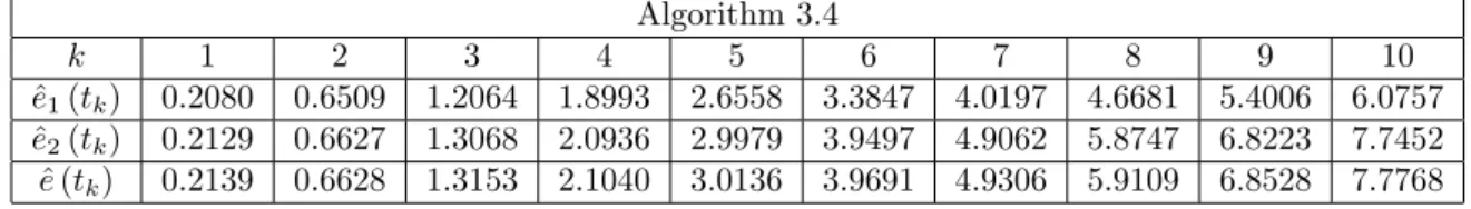
The exact solution (21) gives us a benchmark to Algorithm 3.4 with respect to a finite difference method [13, 14]. As in [13], we estimate numerically (21) with viscosity parameter 𝜈 = 1. We apply Algorithm 3.4 by using the truncation parameter 𝑁 = 6, time-step ℎ = 1/40, space-discretization step 𝛿 = 𝜋/126 and 𝑄 = 6 quantization points, until a final time 𝑇 = 10ℎ. We compute the term Q̂︀𝑁 by taking a left Riemann sum approximation of the integrals using 𝑁𝑅 = 𝑁 3− 1 3𝑁 𝜏 = 18 uniform subintervals of [︀ 1 3𝑁, 𝑁
3]︀. Table 1 depicts the numerical results. The
discretization steps are related linearly, instead of the restrictive assumption ℎ = 𝒪 (𝛿2) in the
Algorithm 3.4 𝑘 1 2 3 4 5 6 7 8 9 10 ^ 𝑒1(𝑡𝑘) 0.2080 0.6509 1.2064 1.8993 2.6558 3.3847 4.0197 4.6681 5.4006 6.0757 ^ 𝑒2(𝑡𝑘) 0.2129 0.6627 1.3068 2.0936 2.9979 3.9497 4.9062 5.8747 6.8223 7.7452 ^ 𝑒 (𝑡𝑘) 0.2139 0.6628 1.3153 2.1040 3.0136 3.9691 4.9306 5.9109 6.8528 7.7768
Table 1: Estimation errors ˆ𝑒 (𝑡𝑘) := 𝑒 (𝑡𝑘) · 103 and ˆ𝑒𝑖(𝑡𝑘) := 𝑒𝑖(𝑡𝑘) · 103 to the two-dimensional
Taylor-Green vortex performed by Algorithm 3.4 with 𝑁 = 6, ℎ = 1/40, 𝛿 = 𝜋/126, 𝑄 = 6 and 𝑁𝑅= 18.
4.2
Beltrami flows
The Beltrami flows, introduced by E. Beltrami in 1889 [3], are the ones for which the vorticity vector 𝜔 = curl 𝑢, with rotational operator curl :=∇×, satisfies 𝜔 = 𝜆𝑢 for some parameter 𝜆. That is, the vorticity and the velocity vectors are aligned, or well the velocity is an eigenfunction of the rotational operator.
4.2.1 Three-dimensional Beltrami flow
In particular, we study the three-dimensional viscous Beltrami flow {︃𝑢 (𝑡, 𝑥) = 𝑔 (𝑥) 𝑒−𝜈𝜆2𝑡 , 𝑝 (𝑡, 𝑥) = 𝑝𝑠− 𝜌 [︁‖𝑢(𝑡,𝑥)‖2 2 + g𝑥3 ]︁ , (22)
with non-divergence initial velocity field ⎧ ⎪ ⎪ ⎪ ⎪ ⎨ ⎪ ⎪ ⎪ ⎪ ⎩ 𝑔1(𝑥) = − 𝐴
𝑘2+ ℓ2 [𝜆ℓ cos (𝑘𝑥1) sin (ℓ𝑥2) sin (𝑚𝑥3) + 𝑚𝑘 sin (𝑘𝑥1) cos (ℓ𝑥2) cos (𝑚𝑥3)] ,
𝑔2(𝑥) =
𝐴
𝑘2+ ℓ2 [𝜆𝑘 sin (𝑘𝑥1) cos (ℓ𝑥2) sin (𝑚𝑥3) − 𝑚ℓ cos (𝑘𝑥1) sin (ℓ𝑥2) cos (𝑚𝑥3)] ,
𝑔3(𝑥) = 𝐴 cos (𝑘𝑥1) cos (ℓ𝑥2) sin (𝑚𝑥3) ,
where 𝑥 = (𝑥1, 𝑥2, 𝑥3) ⊤
, 𝑝𝑠 ≥ 0 a time-independent stagnation pressure at ground level, 𝐴 the
amplitude of the vertical velocity and Beltrami coefficient 𝜆 =√𝑘2+ ℓ2+ 𝑚2.
Here, g > 0 is the acceleration due to gravity and 𝜌 > 0 is the density of the fluid which is assumed, as the kinematic viscosity 𝜈 > 0, to be constant. The Beltrami flow (22) solves the in-compressible Navier-Stokes equations (1) with 𝜈 > 0, external force field 𝑓 (𝑡, 𝑥) = −g (0, 0, 1)⊤ and initial divergence-free vector field 𝑔 (𝑥) as above (see [61]). Defining the potential 𝜑 (𝑡, 𝑥) = −g𝑥3, observe that 𝑓 (𝑡, 𝑥) = ∇𝜑 (𝑡, 𝑥). Thus, the constant density 𝜌 > 0 and the conservative
external force field 𝑓 are considered as part of the pressure term 𝑝 (𝑡, 𝑥). That is {︃𝑢 (𝑡, 𝑥) = 𝑔 (𝑥) 𝑒−𝜈𝜆2𝑡 , 𝑝 (𝑡, 𝑥) = 𝑝𝑠 𝜌 − [︁‖𝑢(𝑡,𝑥)‖2 2 + g𝑥3− 𝜑 (𝑡, 𝑥) ]︁ = 𝑝𝑠 𝜌 − ‖𝑢(𝑡,𝑥)‖2 2 , (23)
for 𝑡 ∈ [0, 𝑇 ] and 𝑥 ∈[︀0,2𝜋𝑘]︀×[︀0,2𝜋ℓ ]︀×[︀0,2𝜋𝑚]︀, solves the incompressible Navier-Stokes equations (1) with viscosity parameter 𝜈 > 0 and external force 𝑓 ≡ 0.
We test Algorithm 3.4 by solving the Beltrami flow (23) with different combinations of the parameters 𝜈 > 0, 𝐴 > 0 and 𝑘 = ℓ = 𝑚 = 1 until a final time 𝑇 > 0. For these simulations, the
Reynolds number is in the range [1, 200]. The parameters are described below. The time-step and the final time are such that the exponential damping factor cannot be neglected.
First, we perform one-step in time estimations by taking discretization steps 0 < 𝛿 = 𝑁2𝜋
𝛿 <
ℎ = 𝑁𝑇
ℎ with 𝑁ℎ = 1. As in the two dimensional context, we fix the truncation parameter
𝑁 = 6 and numerical quantities 𝑄 = 6 and 𝑁𝑅 = 18. Table 2 depicts the estimation errors.
Observe the influence of the viscosity 𝜈 > 0 and the velocity amplitude parameter 𝐴 > 0 to the quality of aproximations.
𝜈 𝐴 ℎ 𝑁𝛿 𝑒1(ℎ) 𝑒2(ℎ) 𝑒3(ℎ) 𝑒 (ℎ) 0.005 0.5 0.1 63 0.0000807 0.0000707 0.0000994 0.000127 0.005 1 0.1 63 0.00117 0.000777 0.00130 0.00136 0.005 2 0.1 63 0.01234 0.01083 0.01867 0.01909 0.005 5 0.1 63 0.6691 0.5030 0.94500 0.9840 0.01 0.5 0.1 63 0.0001203 0.0001317 0.0001631 0.0001869 0.01 1 0.1 63 0.001217 0.0008113 0.001019 0.001809 0.01 2 0.1 63 0.01352 0.01183 0.01888 0.01912 0.01 5 0.1 63 0.6216 0.4888 0.9545 0.9903 0.1 0.5 0.2 40 0.0009937 0.0007624 0.0006606 0.0011590 0.1 1 0.2 40 0.0046 0.0029 0.0046 0.0055 0.1 2 0.2 40 0.0439 0.0265 0.0635 0.0654 0.1 5 0.2 40 4.0336 2.4247 5.8554 5.8991 0.1 0.5 0.1 63 0.0003391 0.0002831 0.0002316 0.0004004 0.1 1 0.1 63 0.001482 0.001242 0.002362 0.002489 0.1 2 0.1 63 0.016590 0.010939 0.019589 0.020716 0.1 5 0.1 63 0.5767 0.4280 0.8913 0.9089 1 0.5 0.2 40 0.0056 0.0035 0.0042 0.0062 1 1 0.2 40 0.0180 0.0160 0.0203 0.0247 1 2 0.2 40 0.0928 0.0575 0.0798 0.0988 1 5 0.2 40 1.0389 1.0320 1.1466 1.6058 1 0.5 0.1 63 0.0015 0.0023 0.0024 0.0028 1 1 0.1 63 0.0075 0.0085 0.0118 0.0136 1 2 0.1 63 0.0401 0.0423 0.0514 0.0612 1 5 0.1 63 0.5353 0.3616 0.4363 0.6380 1 1 0.05 126 0.0025 0.0027 0.0033 0.0037 1 5 0.05 126 0.1557 0.1317 0.1640 0.1816 1 1 0.04 158 0.0016 0.0018 0.0026 0.0027 1 5 0.04 158 0.1177 0.0844 0.1293 0.1353 1 1 0.025 252 0.00073 0.00069 0.00095 0.00098 1 5 0.025 252 0.0476 0.0386 0.0599 0.0602
Table 2: One-step in time estimation errors of the Algorithm 3.4 (ℎ > 0 and 𝛿 = 𝑁2𝜋
𝛿 > 0) for
the numerical solution of the Beltrami flow (23) (𝜈 > 0, 𝐴 > 0, 𝑘 = 𝑙 = 𝑚 = 1).
Now, we consider the numerical approximation of the 3𝑑 space-periodic velocity field 𝑢 of the Beltrami flow (23) with 𝜈 = 0.1, 𝐴 = 0.5, 𝑘 = ℓ = 𝑚 = 1 until the final time 𝑇 = 2. Note that the parameters 𝜌, g and 𝑝𝑠 have no influence on the results. In this case, the exponential
factor reduces the magnitude of the initial velocity field until about 54.88%. Table 3 shows the performance of Algorithm 3.4 with truncation parameter 𝑁 = 6, time-step ℎ = 𝑇 /10, spatial discretization 𝛿 = 𝜋/20, 𝑄 = 6 quantization points and 𝑁𝑅 = 18 subintervals to the Riemann
sum estimations.
Finally, we numerically solve of the 3𝑑 space-periodic velocity field 𝑢 of the Beltrami flow (23) with 𝜈 = 0.1, 𝐴 = 1, 𝑘 = ℓ = 𝑚 = 1 until 𝑇 = 1. Observe that the exponential factor reduces the magnitude of the initial velocity field until about 74.08%. Table 4 shows the performance of Algorithm 3.4 with 𝑁 = 6, ℎ = 𝑇 /10, 𝛿 = 2𝜋/63, 𝑄 = 6 and 𝑁𝑅= 18.
Algorithm 3.4 𝑘 1 2 3 4 5 6 7 8 9 10 ˜ 𝑒1(𝑡𝑘) 0.0994 0.2719 0.5046 0.7557 1.0427 1.3278 1.6278 1.8934 2.1408 2.3464 ˜ 𝑒2(𝑡𝑘) 0.0762 0.2097 0.3906 0.5483 0.7490 0.8825 1.0559 1.2134 1.3037 1.3780 ˜ 𝑒3(𝑡𝑘) 0.0661 0.1944 0.3166 0.4872 0.6616 0.7902 1.0241 1.1166 1.2321 1.3769 ˜ 𝑒 (𝑡𝑘) 0.1159 0.2954 0.5503 0.8002 1.1048 1.4035 1.6854 1.9386 2.1779 2.4098
Table 3: Estimation errors ˜𝑒 (𝑡𝑘) := 𝑒 (𝑡𝑘) · 102 and ˜𝑒𝑖(𝑡𝑘) := 𝑒𝑖(𝑡𝑘) · 102 to the three-dimensional
Beltrami flow (23) (𝜈 = 0.1, 𝐴 = 0.5, 𝑘 = 𝑙 = 𝑚 = 1) by using Algorithm 3.4 (𝑁 = 6, ℎ = 1/5, 𝛿 = 𝜋/20, 𝑄 = 6 and 𝑁𝑅 = 18).
Figure 1: Initial velocity field to the three-dimensional Beltrami flow (22) with 𝜈 = 0.1, 𝐴 = 1 and 𝑘 = ℓ = 𝑚 = 1. Algorithm 3.4 𝑘 1 2 3 4 5 6 7 8 9 10 ˜ 𝑒1(𝑡𝑘) 0.1482 0.4451 0.8280 1.3023 1.7570 2.3748 2.9724 3.6903 4.3578 5.0886 ˜ 𝑒2(𝑡𝑘) 0.1242 0.3675 0.6741 1.0009 1.4126 1.8552 2.3155 2.9924 3.5432 4.1730 ˜ 𝑒3(𝑡𝑘) 0.2362 0.7134 1.3252 2.0755 2.9842 3.9512 4.9251 5.9950 7.0374 7.9639 ˜ 𝑒 (𝑡𝑘) 0.2489 0.7825 1.4721 2.3394 3.2192 4.2533 5.2970 6.3564 7.3176 8.2782
Table 4: Estimation errors ˜𝑒 (𝑡𝑘) := 𝑒 (𝑡𝑘) · 102 and ˜𝑒𝑖(𝑡𝑘) := 𝑒𝑖(𝑡𝑘) · 102 to the three-dimensional
Beltrami flow (23) (𝜈 = 0.1, 𝐴 = 1, 𝑘 = 𝑙 = 𝑚 = 1) by using Algorithm 3.4 (𝑁 = 6, ℎ = 1/10, 𝛿 = 2𝜋/63, 𝑄 = 6 and 𝑁𝑅= 18).
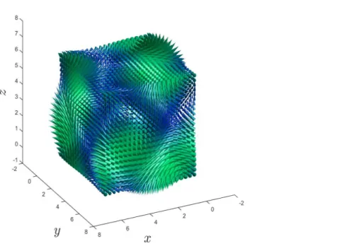
Figure 2: Initial velocity field to the three-dimensional ABC flow (24) with 𝜈 = 0.01 and 𝐴 = 𝐵 = 𝐶 = 0.5.
4.2.2 Arnold-Beltrami-Childress flow
Now, we consider the Arnold-Beltrami-Childress flow [44] ⎧ ⎪ ⎪ ⎪ ⎨ ⎪ ⎪ ⎪ ⎩
𝑢1(𝑡, 𝑥) = (𝐴 sin (𝑥3) + 𝐶 cos (𝑥2)) exp (−𝜈𝑡) ,
𝑢2(𝑡, 𝑥) = (𝐵 sin (𝑥1) + 𝐴 cos (𝑥3)) exp (−𝜈𝑡) ,
𝑢3(𝑡, 𝑥) = (𝐶 sin (𝑥2) + 𝐵 cos (𝑥1)) exp (−𝜈𝑡) ,
𝑝 (𝑡, 𝑥) = − (𝐵𝐶 cos (𝑥1) sin (𝑥2) + 𝐴𝐵 sin (𝑥1) cos (𝑥3) + 𝐴𝐶 sin (𝑥3) cos (𝑥2)) exp (−2𝜈𝑡) + 𝑐,
(24) for (𝑡, 𝑥) ∈ [0, 𝑇 ] × [0, 2𝜋]3, with final time 𝑇 > 0, parameters 𝐴, 𝐵, 𝐶 ∈ R and constant 𝑐 ∈ R. The ABC flow was introduced by Arnold [2] and Childress [11] as a class of Beltrami flow (with Beltrami coefficient 𝜆 = 1). The three-dimensional velocity field 𝑢 and pressure term 𝑝 defined by (24) solve the incompressible Navier-Stokes equations (1) with viscosity parameter 𝜈 > 0 and external force 𝑓 ≡ 0. In our simulations, we consider a Reynolds number in the range [1, 100].
We examine the ABC flow (24) with 𝜈 = 1 and 𝐴 = 𝐵 = 𝐶 = 1 until a final time 𝑇 > 0. The Algorithm 3.4 is performed to obtain one-step in time estimations (that is 𝑇 = ℎ) by using the time steps ℎ = 1/10, 1/20, 1/30, 1/40 and the space discretizations 𝛿 = 2𝜋/63, 2𝜋/126, 2𝜋/189, 2𝜋/252, respectively. The estimation errors result
𝑒 (ℎ) = 4.3185 · 10−2, 1.1998 · 10−2, 5.2584 · 10−3, 3.3223 · 10−3,
respectively. As above we have set the parameters 𝑁 = 6, 𝑄 = 6 and 𝑁𝑅 = 18. Observe
the better results as the time-space grid increases its quantity of nodes. The order of error estimations results similar as in the case of the discontinuous Galerkin method presented in [65].
Finally, we simulate the ABC flow (24) with 𝜈 = 0.01 and 𝐴 = 𝐵 = 𝐶 = 0.5 until 𝑇 = 7/10. Table 5 presents the estimation errors of Algorithm 3.4 with truncation parameter
Algorithm 3.4 𝑘 1 2 3 4 5 6 7 8 9 10 ˜ 𝑒1(𝑡𝑘) 0.0400 0.1449 0.3178 0.5553 0.8433 1.1800 1.5744 2.0311 2.5400 3.0662 ˜ 𝑒2(𝑡𝑘) 0.0574 0.1990 0.4256 0.7479 1.1740 1.6526 2.3021 2.9373 3.8502 4.6322 ˜ 𝑒3(𝑡𝑘) 0.0427 0.1564 0.3434 0.5954 0.9202 1.3296 1.8393 2.3489 3.0317 3.7326 ˜ 𝑒 (𝑡𝑘) 0.1001 0.3661 0.8010 1.3877 2.1203 3.0003 4.1640 5.2858 6.9379 8.6758
Table 5: Estimation errors ˜𝑒 (𝑡𝑘) := 𝑒 (𝑡𝑘) · 102 and ˜𝑒𝑖(𝑡𝑘) := 𝑒𝑖(𝑡𝑘) · 102 to the three-dimensional
ABC flow (24) (𝜈 = 0.01, 𝐴 = 𝐵 = 𝐶 = 0.5) by using Algorithm 3.4 (𝑁 = 6, ℎ = 7/100, 𝛿 = 𝜋/45, 𝑄 = 6 and 𝑁𝑅 = 18).
𝑁 = 6, time-step ℎ = 𝑇 /10, spatial discretization 𝛿 = 𝜋/45, 𝑄 = 6 quantization points and 𝑁𝑅= 18 subintervals to the Riemann sum estimations.
5
Conclusions
Forward-backward SDEs driven by Brownian motion are linked to nonlinear PDEs by means of the Feynman-Kac formula. The deterministic solution is interpreted as the conditional expectation of a diffusion process, and a stochastic algorithm to compute estimations is deduced from its probabilistic representation. A novel system of FBSDEs due to F. Delbaen, J. Qiu and S. Tang [26] introduces a probabilistic approach associated to the incompressible Navier-Stokes equations in dimensions 𝑑 = 2, 3. The Burgers equation is bounded to Itô and Backward SDEs on [0, 𝑇 ]. Then the pressure term and the incompressibility condition are incorporated by an additional BSDE on the time interval (0, +∞). Therefore an estimation of the velocity field that solves the unsteady Navier-Stokes equations follows from the numerical simulation of stochastic particles governed by a coupled forward-backward SDEs system (FBSDS) driven by independent Brownian motions.
Motivated by Delbaen et al. the infinite interval of the extra BSDE is truncated to[︀1 𝑁, 𝑁]︀;
with 𝑁 ∈ N, thus the velocity field is approximated by 𝑢𝑁. The resulting FBSDEs system
is computationally simulated by positioning particles onto an uniform temporal-spatial grid with discretization parameters in time ℎ > 0 and space 𝛿 > 0 such that ℎ, 𝛿 ∈ (0, 1). The forward-backward SDEs are numerically solved by using a methodology in the spirit of Delarue and Menozzi [24] i.e. by means a local discretization in time and taking Euler type integra-tion schemes and optimal quantizers to the Wiener increments to approximate the condiintegra-tional expectations on each temporal-spatial node. The pressure term demands to solve the BSDE associated to its Poisson problem, and the approximation of expectations of integrals involving path of Brownian motions appears as an additional challenge. As in [24], the spatial steps are considered 𝛿 < ℎ. Moreover we have taken 𝛿 < √1
𝑁 to capture the local perturbations for
solving the extra BSDE. In our numerical tests, the quantization of the underlying Gaussian processes together with a Riemann sum estimation of integrals appear as a good approach to deal with this problem. The integrals on the truncated interval [︀3𝑁1 ,𝑁3]︀ are approximated by taking Riemann sum approximations with step sizes 𝜏 ∈ (0, 1).
In this work, we study the numerical simulation of spatially periodic solutions to the Navier-Stokes equations. We present a two dimensional Taylor-Green vortex simulation with order 10−3 estimation errors to the velocity field. Moreover we report numerical results on three dimensional Beltrami flows achieving order 10−2 for the approximation errors. The quantity of particles increases as the space dimension grows, and additional computation is demanded to simulate the exact solutions. Moreover, from Morrey’s inequality
𝐻𝑚 ⊂ 𝐶𝑚−[𝑑2]−1,𝛼
with Hölder exponent 𝛼 = 12 when 𝑑 = 3 or any number 𝛼 ∈ (0, 1) if 𝑑 = 2. Observe a loss of accuracy to the order of estimation 𝒪(︀1/𝑁𝛼4)︀ in the three dimensional context, hence the
truncation parameter 𝑁 must increases to obtain theoretical errors as in the two dimension case.
The expected values are computed by replacing the underlying Gaussian random variables with optimal quantizers of the Normal distribution available in the website [20]. In practice, the quantization approach presents an advantage to the traditional Monte Carlo simulation because its non-asymptotic error bound of estimation 𝒪(︁1/𝑄1𝑑
)︁
. Given a codebook of size 𝑄, the quantization error is better in low dimension. We consider a few quantizer points instead of the usage of many independent realizations of random variables.
We report numerical results by using the truncation parameter 𝑁 = 6 and 𝑄 = 6 optimal quantizer points in two and three dimensions. The Riemann sum estimations on the interval [︀ 1
3𝑁, 𝑁
3]︀ are computed by using the uniform discretization step 𝜏 = (︀ 𝑁
3 − 1
3𝑁)︀ /𝑁𝑅 with 𝑁𝑅 =
18 subintervals. The Euler-Maruyama method is considered to approximate the Itô SDEs components with additive noise 𝜈 ∈ {1, 0.1, 0.01, 0.005}. The time discretization step is essential to the performance of numerical solutions. It is well-known that Euler-Maruyama scheme could not be appropriate for turbulent flows as in the case of passive tracers model with low viscosity parameter. A convenient numerical scheme needs to be considered in the case of vanishing viscosity (see e.g. [60]).
The rate of convergence of Algorithm 3.4 depends on the initial data 𝑓 , 𝑔 and 𝜈 > 0, the parameter 𝑁 , the discretization steps on [0, 𝑇 ], R𝑑 and [︀3𝑁1 ,𝑁3]︀, and the optimal quantization of the independent Brownian motions 𝑊 and 𝐵. Roughly we have
⃦ ⃦𝑢 − ¯𝑢𝑁⃦⃦≤ ⃦ ⃦𝑢 − 𝑢𝑁⃦⃦+ ⃦ ⃦𝑢𝑁 − ¯𝑢𝑁⃦⃦= 𝒪 (︂ 1 𝑁𝛼4 )︂ + error (𝑁, ℎ, 𝛿, 𝜏, 𝑄) ,
with 𝛼 depending on 𝑑 ∈ {2, 3}. The estimation error involves the dimension 𝑑 and the 𝛼-Hölder regularity. The reported numerical tests motivate the theoretical study and numer-ical analysis of the probabilistic methodology associated to the incompressible Navier-Stokes equations. Moreover they suggest the extension of variance reduction methods to contexts as computing conditional expectations to solve systems of FBSDEs. Dealing with more general boundary conditions will be subject to future works.
Acknowledgements
H. Mardones González thanks the funding of the Becas Chile, CONICYT grant, Chile, and the partial support by research team TOSCA, INRIA Nancy Grand Est, France, and ANESTOC TOSCA associated team INRIA project.
References
[1] F. Antonelli. Backward-forward stochastic differential equations. Ann. Appl. Probab., 3:777–793, 1993.
[2] V. I. Arnold. Sur la topologie des écoulements stationnaires des fluides parfaits. C. R. Acad. Sc. Paris, 261:17–20, 1965.
[3] Eugenio Beltrami. Considerations on Hydrodynamics. Int. J. Fusion Energy, 3:53–57, 1985. Translated by Dr. Giuseppe Filipponi from original paper appeared in 1889 in Rendiconti del Reale Instítuto Lombardo, Series II, Vol. 22.