Simulations of the last interglacial and the subsequent glacial inception with the Planet Simulator

(1)

HAL Id: hal-00298166

https://hal.archives-ouvertes.fr/hal-00298166

Submitted on 13 Dec 2006

HAL is a multi-disciplinary open access

archive for the deposit and dissemination of sci-entific research documents, whether they are pub-lished or not. The documents may come from teaching and research institutions in France or abroad, or from public or private research centers.

L’archive ouverte pluridisciplinaire HAL, est destinée au dépôt et à la diffusion de documents scientifiques de niveau recherche, publiés ou non, émanant des établissements d’enseignement et de recherche français ou étrangers, des laboratoires publics ou privés.

Simulations of the last interglacial and the subsequent

glacial inception with the Planet Simulator

M. Donat, F. Kaspar

To cite this version:

M. Donat, F. Kaspar. Simulations of the last interglacial and the subsequent glacial inception with the Planet Simulator. Climate of the Past Discussions, European Geosciences Union (EGU), 2006, 2 (6), pp.1347-1369. �hal-00298166�

(2)

CPD

2, 1347–1369, 2006

Simulating last interglacial and glacial inception

M. Donat and F. Kasper

Title Page Abstract Introduction Conclusions References Tables Figures ◭ ◮ ◭ ◮ Back Close

Full Screen / Esc

Printer-friendly Version Interactive Discussion

EGU Clim. Past Discuss., 2, 1347–1369, 2006

www.clim-past-discuss.net/2/1347/2006/ © Author(s) 2006. This work is licensed under a Creative Commons License.

Climate of the Past Discussions

Climate of the Past Discussions is the access reviewed discussion forum of Climate of the Past

Simulations of the last interglacial and the

subsequent glacial inception with the

Planet Simulator

M. Donat and F. Kaspar

Freie Universit ¨at Berlin, Institut f ¨ur Meteorologie, Berlin, Germany

Received: 16 November 2006 – Accepted: 7 December 2006 – Published: 13 December 2006 Correspondence to: M. Donat ([email protected])

(3)

CPD

2, 1347–1369, 2006

Full Screen / Esc

EGU

Abstract

The Planet Simulator was used to perform equilibrium simulations of the Eemian inter-glacial at 125 kyBP and the inter-glacial inception at 115 kyBP. Additionally, an accelerated transient simulation of that interval was performed. During this period the changes of Earth’s orbital parameters led to a reduction of summer insolation in the northern

5

latitudes. The model has been run in different configurations in order to evaluate the influence of the individual sub-models. The strongest reaction on the insolation change was observed when the atmosphere was coupled with all available sub-systems: a mixed-layer ocean and a sea-ice model as well as a vegetation model. In the simula-tions representing the interglacial, the near-surface temperature in northern latitudes

10

is higher compared to the preindustrial reference run and almost no perennial snow cover occurs. In the run for the glacial inception, wide areas in mid and high northern latitudes show negative temperature anomalies and wide areas are covered by snow or ice. The transient simulation shows that snow volume starts to increase after sum-mer insolation has fallen below a critical value. The main reason for the beginning

15

glaciation is the locally reduced (summer) temperature as a consequence of reduced summer insolation. Therefore, a larger fraction of precipitation falls as snow and less snow can melt. That mechanism is amplified by the snow-albedo-feedback.

1 Introduction

According toMilankovich(1941), variations of the Earth’s orbit lead to changes in

inso-20

lation. He suggested that decreased insolation in high latitudes during summer would be the most important factor for a glacial inception.

In this study the Planet Simulator1(Fraedrich et al.,2005), a general circulation model (GCM) of reduced complexity has been applied to simulate the climate of the Eemian interglacial (125 kyBP) and the subsequent glacial inception (115 kyBP). These dates

25

1

(4)

CPD

2, 1347–1369, 2006

Full Screen / Esc

EGU represent periods with increased and weakened seasonality of insolation on the

north-ern hemisphere, caused by a change of the orbital parameters (Berger, 1978). At 125 kyBP insolation in mid and high northern latitudes during (northern) summer was significantly higher compared to present day values; in winter it was lower. At 115 kyBP seasonality of northern hemispheric insolation was reduced. Insolation was

signifi-5

cantly lower than today in mid and high northern latitudes during (northern) summer and was higher during winter. For a detailed discussion of insolation patterns during interglacials seeBerger et al.(2006).

A set of experiments with different models have already been performed to simu-late the transition from the simu-latest interglacial period into the subsequent glacial period.

10

Atmosphere-only-GCMs which were used in early experiments failed to successfully simulate a glacial inception. For a detailed review see Vettoretti and Peltier (2004). Khodri et al. (2001) as well as Vettoretti and Peltier (2003) performed experiments with coupled atmosphere-ocean models. Both studies came to the conclusion that the ocean acts as a positive feedback mechanism for glacial inception. Without such

15

a feedback, models do not succeed in simulating an significant increase of the snow-and ice-cover in high northern latitudes. Recent experiments with coupled GCMs ( Kas-par and Cubasch,2006) and also EMICs (Kubatzki et al.,2006) showed that models succeed to simulate the glacial inception when the atmosphere is coupled to an ocean-or ice-sheet-model. However, the application of various types of models led to

differ-20

ent conclusions about details of the glaciation process. It is therefore of interest to compare the behaviour of diverse models. Compared to other types of models the Planet Simulator combines several advantages. Compared to typical EMICs, the at-mospheric component is more comprehensive (Fraedrich et al.,2005), operates with more regional details and is therefore more similar to a GCM. Compared to GCMs, the

25

Planet Simulator has the advantage that it allows to couple different sub-systems and that it is computational much more efficient. It can therefore be used to run large sets of sensitivity experiments.

(5)

CPD

2, 1347–1369, 2006

Full Screen / Esc

EGU

2 Model description and experimental setup

The central component of the Planet Simulator is an atmospheric GCM, that solves the basic dynamics. The applied version operates at a resolution of T21 (approx. 5.6◦₎ and on 5 vertical levels. The dynamical core of the Planet Simulator is based on the moist primitive equations representing the conservation of momentum, mass and

en-5

ergy (Fraedrich et al.,2005). The set of equations consists of prognostic equations for the vertical component of the vorticity and the horizontal divergence, the first law of thermodynamics, equation of state (with hydrostatic approximation), continuity equa-tion and a prognostic equaequa-tion for water vapour (specific humidity). The atmosphere can be coupled to a mixed-layer ocean, a sea-ice model and a vegetation model. The

10

Planet Simulator has been developed at the University of Hamburg and has been de-signed as an efficient tool to run simulations with low computing costs. On a standard single-CPU PC (Intel Pentium 4, 2.4 GHz) about 100 years can be simulated per day. Thus, it is possible to run a number of experiments and also a transient simulation of the 10 000 year period.

15

Sensitivity tests with different configurations of the model have been performed in order to explore the influence of the sub-models. Table1gives an overview of the simulations and their configuration. The orbital parameters and thus the insolation are calculated according toBerger (1978) and refer to the year 1950. For each configuration, three simulations were performed: one with the insolation of 125 000 years BP (hereafter

20

labelled with 125 ky ), another with insolation of 115 000 years BP (115 ky ) and as preindustrial reference a run with today’s insolation (REF ). The latter is approximately equal to preindustrial values due to the relatively long periods of the varying orbital parameters. The atmospheric CO2 concentration was fixed to a preindustrial value of 270 ppm in all simulations in order to allow ascribing the simulated climatic

anoma-25

lies to the changed orbital parameters. Moreover, this is justifiable because the CO2 concentrations differ only slightly at the three regarded periods (Petit et al.,1999).

(6)

CPD

2, 1347–1369, 2006

Full Screen / Esc

EGU

3 Influence of the coupled sub-systems

The simulations in this and the following section were performed as equilibrium runs. Compared to more complex climate models, the Planet Simulator reaches an equilib-rium state relatively fast. In the simulations with not more than one coupled sub-model an equilibrium was reached within 20 years. These experiments were performed for

5

50 years in order to have a stable period for calculating climatological means. The sta-bilization took longer when the atmospheric component was coupled to the vegetation model in combination with the ocean and sea-ice model. Therefore, these simulations were carried out for 300 years.

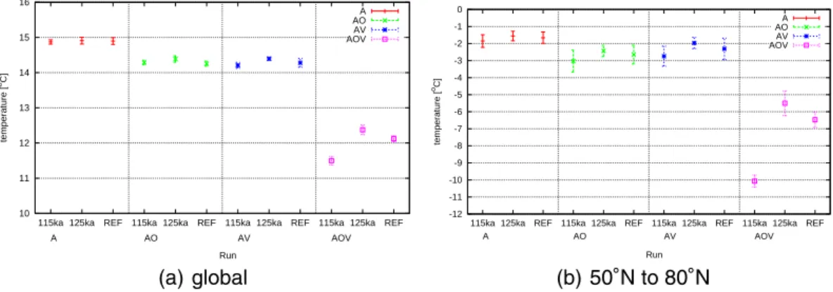
Figure 1 shows the global mean temperatures of the different simulations. When

10

only one of the subsystems is coupled, the model reacts with a temperature reduction for all periods. However, when all subsystems are active the reaction is much stronger than the sum of the single effects. This illustrates the nonlinearity of the system.

At least slightly lower temperatures are simulated for 115 kyBP in all experiments in

15

which the atmosphere is coupled to one or more sub-models (compared to 125 kyBP and the reference run). Only the experiment with the uncoupled atmosphere produces almost identical temperature values for the different insolation conditions. This confirms the experiences that without an additional feedback the atmosphere-only-GCM will not succeed in simulating the cold state. The configuration with all sub-systems activated

20

shows the strongest reaction on the change in insolation and results in a difference of 0.7 K in the global mean temperature between 125 ky and 115 ky.

If the calculation of the mean temperature is restricted to the mid and high northern lat-itudes (50◦_N–80◦

N), the differences between the simulations are significantly greater. For example, in the AOV-configuration a difference of more than 4 K between 125 ky

25

and 115 ky is simulated for this region.

In the following section we analyze the simulated climate for the different periods in detail. The focus is on the simulations with all sub-models activated (AOV), i.e. in which

(7)

CPD

2, 1347–1369, 2006

Full Screen / Esc

EGU the largest differences in simulated temperatures occur.

4 Detailed analysis of the simulated climates in the equilibrium runs

The results presented in this section are all based on the last 30 years of the AOV-simulations. Thus, the values are considered as climatological means of the equilibrium states.

5

4.1 Near-surface temperature

Globally and on the northern hemisphere, the annual cycle of the near-surface temperature (not shown) reflects the seasonal distribution of insolation. While for the 125 ky -run the seasonal difference of the global mean temperature is approximately 5 K, the difference between summer and winter temperature is less than 3 K for the 115 ky-run,

10

associated with a considerably lower (northern) summer temperature (approximately 2 K cooler than 125 ky ). This stronger seasonality for 125 ky can also be seen when only the northern hemisphere or especially the high northern latitudes are regarded. In these latitudes, during all months of the year the temperatures of the 115 ky -run are lower than those of the 125 ky -run, even during the winter months, when insolation is

15

higher. One reason for this is the wider snow cover in this area which will be analyzed later in this text.

In Fig.2 the global distribution of the annual and seasonal (DJF, JJA) temperature anomalies of the runs 115 ky and 125 ky are shown relative to the preindustrial refer-ence REF. The temperatures differ between the simulations particularly on the northern

20

hemisphere, and here especially over land areas.

The annual means of the 125 ky -run show positive temperature anomalies of 1 to 2 K over wide continental parts and the Arctic region, while the land areas in the equatorial regions are cooler. Temperature anomalies over the ocean areas are smaller.

During the (northern) summer months (JJA) the temperature is higher over all

(8)

CPD

2, 1347–1369, 2006

Full Screen / Esc

EGU nents, compared to the preindustrial reference (Fig.2c). This is a direct consequence

of the stronger insolation (because of the reduced distance between Earth and Sun as well as the stronger obliquity).

During (northern) winter (DJF) most parts of the continental areas respond to the de-crease in insolation – the Earth passes at this time its aphelion – and show lower

5

temperatures compared to the reference run (Fig.2e). Positive temperature anomalies are simulated only northwards of 60◦_{N. They are related to the far lower snow and ice} cover, which will be discussed in the following subsection.

As about 2/3 of the land area are located on the northern hemisphere and the reaction on the modified insolation is much stronger on land than over the (mixed-layer) ocean,

10

temperature anomalies on the northern hemisphere are greater than on southern. In case of the 115 ky -simulation significant cooling occurs at the mid and high north-ern latitudes (Fig.2b). These negative temperature anomalies are not restricted to land areas. Lower temperatures are also simulated over the northern parts of the Pacific and the Atlantic due to the increased permanent sea-ice cover in these regions.

15

The strong negative temperature anomalies in the mid and high northern latitudes are also visible when the means are calculated for the summer and accordingly win-ter months (Fig.2d/f). Northwards of about 40◦

N, temperatures over continents and oceans are lower compared to the preindustrial reference. During the (northern) sum-mer months - when the insolation is lower than in today’s sumsum-mers – this cooling is

par-20

ticularly strong. The anomalies of the winter temperature – when insolation is higher than today – are smaller, but still negative.

Temperature anomalies over the oceans south of about 30◦_{N are mostly less strong} than over land areas also in the 115 ky -simulation. An exception are the Antarctic re-gions of the oceans, where – specially during the southern winter – temperatures are

25

significantly higher over a large area.

Consistent patterns of temperature anomalies can be found in reconstructions. At 125 kyBP Europe and other northern hemispheric continental areas are affected by higher temperatures see e.g. K ¨uhl (2003); Frenzel et al. (1992), while the sea

(9)

sur-CPD

2, 1347–1369, 2006

Full Screen / Esc

EGU face temperatures differ only marginally from preindustrial reference values (CLIMAP,

1984). The lower temperature values for 115 kyBP also agree with reconstructions (Kukla et al.,2002a). A similar global distribution of the temperature was also found in simulations with a more complex coupled GCM for both dates (Kaspar and Cubasch, 2006).

5

4.2 Minimum snow- and sea-ice-cover

The annual minimum of snow- and sea-ice-cover is used here to identify areas with a permanent coverage. These regions play an important role for the accumulation of snow. By increasing the albedo the radiation balance is also changed.

In Fig. 3 the annual minimum snow- and sea-ice-cover is shown for the simulations

10

for 125 ky and 115 ky. In both simulations the Arctic sea is permanently ice-covered, as well as the very Northwest of the Atlantic ocean and parts of the northern Pacific. The high snow cover over Greenland is given by the fixed glacier mask. In the 125 ky -run, besides Greenland, there is almost no perennial snow cover on continental areas (Fig.3a).

15

Compared to that, in the 115 ky -run the permanent sea-ice cover reaches farther to the south. Particularly the permanently ice-covered area of the northern Pacific is much larger and reaches farther to the south (Fig.3b). There is also a larger extent of sea-ice north of Scandinavia. Furthermore, the sea-ice cover of the Arctic Sea is much thicker than in the 125 ky -simulation and additionally covered by snow on wide parts. There

20

are wide perennial snow-covered areas also over the continents in this run. Besides the Himalayan region, this is the case in the Northeast of Asia and of North America. Here, the snow cover extends even in summer until about 50◦_{N southwards.}

In summary, the simulations show a significantly increased permanent snow- and sea-ice-cover on the northern hemisphere for 115 000 years BP, compared to 125 000 years

25

BP. The areas with a perennial snow and ice cover were already identified as regions with particularly large negative temperature anomalies in Sect.4.1. The large extent of snow cover over North America is consistent with reconstructions (Clark et al.,1993).

(10)

CPD

2, 1347–1369, 2006

Full Screen / Esc

EGU However, the perennial snow cover in the Northeast of Asia is not in accordance with

reconstructions (Peltier, 1994). Reconstructions for this region show that, although there was permafrost, no glaciation occurred due to a lack of precipitation. In the simulation, there is an overestimation of precipitation in the Asian region which results in the accumulation of snow.

5

4.3 Development of the permanent snow- and ice-cover in the 115 ky -run

In the 115 ky -simulation less energy is available for absorption on the surface in the high northern latitudes as a consequence of the reduced summer insolation. Thus, the surface temperature is lower and because of the weaker long wave radiation the atmo-spheric layers above are heated less. The lower temperature causes a greater part of

10

precipitation falling as snow, whereof less melts during the cooler summer. Therefore large areas with can be established. Consequently, the surface albedo is increases in these regions and in turn there is again less energy available for heating. Thus, the snow cover can grow and the albedo of the additionally covered area will further increase. This so-called snow-albedo-feedback explains the expansion of snow- and

15

ice-covered areas in the high northern latitudes.

In contrast to that, Kukla et al. (2002b) suggested that the glaciation was caused by the increased temperature gradient between low and high northern latitudes. Consequently, the meridional moisture transport could have been increased. This could have led to the fast build-up of ice-sheets by increased snowfall. However,

20

Kaspar and Cubasch(2006) showed (in their simulations with ECHO-G) that south-wards winds from the north pole lead to an amplified cooling in those regions where the accumulation of snow begins.

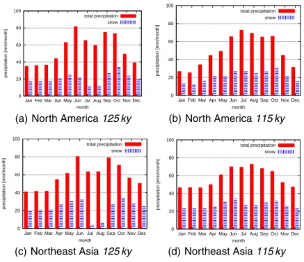
In Fig.4the annual cycle of total precipitation and snowfall is shown for the regions where the snow cover occurs in the 115 ky -simulation. Mean monthly quantities are

25

calculated for a region of the north-east of North America (100◦_{W to 60}◦_{W and 50}◦_N to 80◦_{N) and the northern part of Asia (90}◦_{E to 160}◦_{E and 50}◦_{N to 80}◦_{N). For} com-parison, the same values are calculated for the 125 ky -simulation, in which almost no

(11)

CPD

2, 1347–1369, 2006

Full Screen / Esc

EGU perennial snow cover occurs.

In both simulations and both regions the precipitation maximum occurs during summer and the lowest amount of precipitation in winter. There are no significant differences between both simulations concerning annual precipitation as well as precipitation in summer (JJA) or winter (DJF).

5

In the 115 ky -simulation the fraction of precipitation falling as snow is substantially higher during the summer months July and August than in the 125 ky -simulation. So there is in fact more snowfall in the 115 ky -case in those regions where a permanent snow cover establishes, but the total precipitation quantity is not increased. The greater fraction of snow is mainly caused by the lower temperatures (refer Fig.2). The fact that

10

the total precipitation (in areas covered by snow during the glacial inception) shows no significant differences between the different simulations already argues against Kukla’s (2002b) hypothesis. Nevertheless, the meridional moisture transports was also an-alyzed. It is calculated as the product of the meridional wind component v and the specific moisture q (Peixoto and Oort, 1992) in each layer and mass-weighted

verti-15

cally integrated.

The result again shows no significant differences between the simulations for both di-rection and amount of moisture transport. Furthermore, the relevant regions are rather under the influence of southward transports for both annual mean and during summer (when differences in snowfall are highest). The absolute values of the transport are

20

higher over the snow covered areas in North America, while transport is relatively low over Northeast Asia, as there are quite low pressure gradients on average.

In summary, the analysis showed no increase of precipitation in those regions where a permanent snow cover occured in the 115 ky -simulation. The annual mean is in some places even lower compared to the preindustrial reference and the 125 ky

-25

simulation. The comparison of the annual cycles of precipitation for the 115 ky - and the

125 ky -case shows as the most distinctive difference a significant decrease of summer

snowfall for 125 ky, while the fraction of precipitation as snow in the 115 ky -simulation remains relatively high also during the summer months. Overall, there is more

(12)

CPD

2, 1347–1369, 2006

Full Screen / Esc

EGU snowfall in the relevant regions in this simulation. The connection between increased

meridional moisture transport and increased precipitation as suggested byKukla et al. (2002b) as a reason for the increased expansion of snow could not be approved on the basis of this simulations.

Due to the – mainly during the (northern) summer – reduced solar insolation in high

5

northern latitudes, temperature is considerably lower in this region. This leads on the one hand to a greater fraction of precipitation falling as snow and on the other hand to less melting of snow. This effect is furthermore amplified by the snow-albedo-feedback. In some regions the permanent snow cover reaches farther to the south than in other regions. E.g. western Europe is affected by advection of air from the Atlantic ocean.

10

Thus, temperature is higher than in other regions on the same latitudes and no perennial snow cover is established.

5 Transient simulation

Due to the computational efficiency of the Planet Simulator, it is feasible to run a

tran-15

sient simulation of the transition from the interglacial into the glacial. Such a run with a continuous variation of the insolation conditions was performed for the interval from 125 000 years BP until 115 000 years BP, accelerated by a factor of 10. Thus, the real period of 10 000 years was computed within 1 000 simulation years. Such an ac-celeration of the orbital forcing was suggested byJackson and Broccoli (2003) and

20

Lorenz and Lohmann (2004). It can be problematic as the sub-systems might react with different time-lags. Lunt et al.(2006, this special issue) showed that accelerated simulations behave in a damped fashion, but with no phase-lag compared to the non-accelerated simulation. The Planet Simulator typically reaches an equilibrium state much faster than the typical periods of changes in the orbital parameters. Therefore

25

an accelerated simulation is justifiable and allows at least a rough estimation of the transition into the glaciation.

(13)

CPD

2, 1347–1369, 2006

Full Screen / Esc

EGU The temporal development of the global mean temperature and the mean solar

insola-tion during summer (JJA) at 65◦_{N are shown in Fig.} ₅_{together with the temperatures} of the equilibrium runs. Around 125 kyBP summer insolation in the high northern lat-itudes is close to its maximum and starts to decrease. The global mean temperature remains at its maximum values of about 285.5 K until approximately 122 kyBP. Then

5

the temperature starts to decrease until the end of the simulation. It drops to 284.8 K. The difference between the temperatures 125 kyBP and 115 kyBP is slightly smaller than in the equilibrium runs. At 115 kyBP the temperature in the transient simulation is about 0.2 K warmer relative to the equilibrium run. This damped behavior could be due to the acceleration of the boundary conditions, but also just to their transient variation.

10

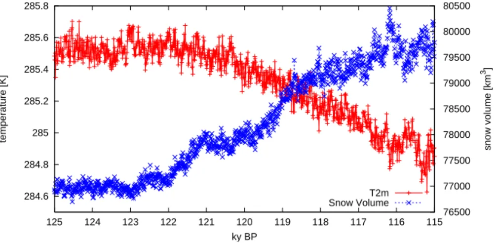
The global snow volume remains initially stable on its minimum. At approx. 123 kyBP it starts to increase significantly, mainly on the northern hemisphere. Until approx. 123 kyBP summer insolation in high northern latitudes is still sufficiently high to pre-vent the accumulation of snow. From then, summer insolation declines below a critical value, an increase of snow volume begins and continues until the end of the

simula-15

tion. With a time lag the described decrease of the global mean temperature begins. The contrary trends of global mean temperature and snow volume are shown in Fig.6. Mean temperature decreases with increasing snow volume.

6 Summary and conclusions

We have applied the Planet Simulator to simulate the climate of the Eemian

inter-20

glacial (125 kyBP) and the subsequent glacial inception (115 kyBP). The simulations have been performed as equilibrium runs and also as a transient simulation, acceler-ated by factor 10. As boundary conditions only orbital parameters were modified and thus, the seasonal and latitudinal distribution of insolation.

The results show that the model is partly successful in qualitatively simulating the

cli-25

matic conditions of these periods in agreement with reconstructions and simulations with more complex AOGCMs.

(14)

CPD

2, 1347–1369, 2006

Full Screen / Esc

EGU The strongest response to the insolation change is simulated when all sub-systems

are activated: the mixed-layer ocean, the sea-ice- and the vegetation model. Thus, the results confirm that additional feedbacks are essential for simulating the expansion of snow cover and the related cooling.

The widest expansion of permanent snow cover in the 115 ky -simulation was found

5

in the northeastern part of North America as well as in the Northeast of Asia. The temperature in mid and high northern latitudes is significantly reduced relative to a ref-erence run under preindustrial conditions. In the 125 ky -simulation the temperatures are higher especially over continental areas and almost no permanent snow cover oc-curs.

10

The expansion of snow cover in the 115 ky -simulation is mainly caused by the lower summer temperatures in high northern latitudes. Consequently, a larger fraction of precipitation falls as snow and less snow can melt. The assumption that the increased meridional temperature gradient leads to a stronger moisture transport and conse-quently to increased snowfall, could not be confirmed with these simulations. In our

15

Planet Simulator experiments for the glacial inception perennial snow cover occurs also over Northeast Asia which is inconsistent to reconstructions. This is caused by an overestimation of precipitation in this region that also occurs in the preindustrial simu-lation. Model experiments with more complex GCMs (Kaspar and Cubasch,2006) or EMICs (Kubatzki et al.,2006) led to a regional distribution of perennial snow cover in

20

better agreement with reconstructions.

The transient simulation of the whole interval from 125 kyBP to 115 kyBP shows that snow volume starts to increase after summer insolation in high northern latitudes falls below a critical value. With increasing snow cover, the global mean temperature de-creases. In the transient simulation the global temperature at 115 kyBP is about 0.2 K

25

warmer than in the equilibrium run.

The simulations with the Planet Simulator show a far minor temperature difference be-tween the selected periods compared to ice-core reconstructions or simulations with more complex models. This might be due to its reduced complexity and also to the

(15)

CPD

2, 1347–1369, 2006

Full Screen / Esc

EGU low resolution applied in this study (approx. 5.6◦_{, 5 vertical levels). However, the main}

results correspond qualitatively to the cited references and thus show that this coupled GCM of reduced complexity is at least capable to provide a rough estimation of the climatic conditions.

Acknowledgements. The Planet Simulator was developed and provided by the

Meteorolog-5

ical Institute of the University of Hamburg, working group Theoretical Meteorology (http:

//www.mi.uni-hamburg.de/plasim). We are especially grateful to F. Lunkeit for his friendly tech-nical support.

References

Berger, A. L.: Long-term variations of daily insolation and Quarternary climate changes, J.

10

Atmos. Sci 35, 2362–2367, 1978.1349,1350

Berger, A. L., Loutre, M.-F., Kaspar, F., and Lorenz, S. J.: Insolation during interglacials, in: The climate of past interglacials, edited by: F. Sirocko, T. Litt, M. Claussen, M. F. S ´anchez-Go ˜ni, Developments in Quarternary Sciences, Vol. 7, Ch. 33, Elsevier, in press, 2006. 1349

Clark, P. U., Clague, J. J., Curry, B. B., Dreimanis, A., Hicock, S. R., Miller, G. H., Berger,

15

G. W., Eyles, N., Lamothe, M., Miller, B. B., Mott, R. J., Oldale, R. N., Stea, R. R., Szabo, J. P., Thorleifson, L. H., and Vincent, J.-S.: Initiation and development of the Laurentide and Cordilleran ice sheets following the last interglaciation, Quaternary Sci. Rev., 12, 79–114, 1993. 1354

CLIMAP Project Members: The last interglacial ocean, Quarternary Research, 21, No. 2, 123–

20

224, 1984.1354

Fraedrich, K., Jansen, H., Kirk, E., Luksch, U., and Lunkeit, F.: The Planet Simulator: Towards a user friendly model, Meteorologische Zeitschrift, 14, 299–304, 2005. 1348,1349,1350

Frenzel, B., Pecsi, M., and Velichko, A. A.: Atlas of paleoclimates and paleoenvironments of the northern hemisphere, Late pleistocene – holocene, Gustav Fischer Verlag, Stuttgart, 1992.

25

1353

Jackson, C. S. and Broccoli, A. J.: Orbital forcing of Arctic climate: mechanisms of climate response and implications for continental glaciation, Clim. Dyn., 21, 539–557, 2003. 1357

(16)

CPD

2, 1347–1369, 2006

Full Screen / Esc

EGU inception with a coupled ocean-atmosphere general circulation model, in: The climate of past

interglacials, edited by: Sirocko, F., Litt, T., Claussen, M., S ´anchez-Go ˜ni, M. F. Developments in Quarternary, Sciences, Vol. 7. Elsevier, in press, 2006. 1349,1354,1355,1359

Khodri, M., Leclaine, Y., Ramstein, G., Braconnot, P., Marti, O., and Cortijo, E.: Simulating the amplification of orbital forcing by ocean feedbacks in the last glaciation, Nature, 410,

5

570–574, 2001. 1349

Kubatzki, C., Claussen, M., Calov, R., and Ganopolski, A.: Modelling the end of an Interglacial (MIS 1, 5, 7, 9, 11), in: The climate of past interglacials, edited by: F. Sirocko, T. Litt, M. Claussen, M.F. S ´anchez-Go ˜ni, Developments in Quarternary Sciences, Vol. 7. Elsevier, in press, 2006. 1349,1359

10

K ¨uhl, N.: Die Bestimmung botanisch-klimatologischer Transferfunktionen und die Rekonstruk-tion des bodennahen Klimazustandes in Europa w ¨ahrend der Eem-Warmzeit, DissertaRekonstruk-tiones Botanicae, 375, pp. 149, 2003.1353

Kukla, G. J.: The Last Interglacial, Science, 287, 987–988, 2000.

Kukla, G. J., Bender, M. L., de Beaulieu; J. L., Bond, G., Broecker, W. S., Cleveringa, P., Gavin,

15

J. E., Herbert, T. D., Imbrie, J., Jouzel, J., Keigwin, L. D., Knudsen, K. L., McManus, J. F., Merkt, J., Muhs, D. R., and M ¨uller, H.: Last Interglacial Climates, Quarternary Research, 58, 2–13, 2002a. 1354

Kukla, G. J., Clement, A. C., Cane, M. A., Gavin, J. E., and Zekiak, S. E.: Last Interglacial and Early Glacial ENSO, Quarternary Research, 58, 27–31, 2002b.1355,1357

20

Lorenz, S. J. and Lohmann, G.: Acceleration technique for Milankovitch type forcing in a cou-pled atmosphere-ocean circulation model: method and application for the Holocene, Clim. Dyn., 23, 727–743, 2004.1357

Lunt, D. J., Williamson, M. S., Valdes, P. J., and Lenton, T. M.: Comparing transient, acceler-ated, and equilibrium simulations of the last 30 000 years with the GENIE-1 model, Climate

25

of the Past, 2, 221–235, special issue on “Modelling Late Quaternary Climate”, 2006. 1357

Milankovich, M.: Kanon der Erdbestrahlung und seiner Anwendung auf das Eiszeitenproblem, Editions Speciales 133, Academie Royal Serbe, 33, pp.633, Belgrade, 1941. 1348

Peixoto, J. P. and Oort, A. H.: Physics of Climate, American Institute of Physics, 1992.1356

Peltier, W. R.: Ice Age Paleotopography, Science, New Series, Vol. 265, No. 5169, 195–201,

30

1994. 1355

Petit, J. R., Jouzel, J., Raynaud, D., Barkov, N. I., Barnola, J. M., Basile, I., Bender, M., Chapel-laz, J., Davis, J., Delaygue, G., Delmotte, M., Kotlyakov, V. M., Legrand, M., Lipenkov, V. M.,

(17)

CPD

2, 1347–1369, 2006

Full Screen / Esc

EGU Lorius, C., Pepin, L., Ritz, C., Saltzman, E., and Stievenard, M.: Climate and atmospheric

history of the past 420 000 years from the Vostok ice core, Nature, 399, 429–436, 1999.

1350

Vettoretti, G. and Peltier, W. R.: Sensitivity of glacial inception to orbital and greenhouse gas climate forcing, Quarternary Science Reviews, 23, 499–519, 2004. 1349

5

Vettoretti, G. and Peltier, W. R.: Post-Eemian Glacial Inception. Part I: The Impact of Summer Seasonal Temperature Bias, Journal of Climate, Vol. 16, No. 6, 889–911, 2003. 1349

(18)

CPD

2, 1347–1369, 2006

Full Screen / Esc

EGU Table 1. Configuration of the equilibrium simulations. In the simulation name “A” stands for

computation of the atmosphere, “O” marks the coupled ocean and sea-ice model. If the vege-tation model is switched on, the name of the simulation contains a “V”.

Simulation Ocean/Sea-Ice Vegetation kyBP atmosphere only, without any coupled sub-models

A/115 ky off off 115

A/125 ky off off 125

A/REF off off 0

atmosphere coupled to mixed-layer ocean and sea-ice model

AO/115 ky on off 115

AO/125 ky on off 125

AO/REF on off 0

atmosphere coupled to vegetation model

AV/115 ky off on 115

AV/125 ky off on 125

AV/REF off on 0

atmosphere coupled to mixed-layer ocean, sea-ice and vegetation model

AOV/115 ky on on 115

AOV/125 ky on on 125

(19)

CPD

2, 1347–1369, 2006

Full Screen / Esc

Printer-friendly Version Interactive Discussion EGU 10 11 12 13 14 15 16 REF 125ka 115ka REF 125ka 115ka REF 125ka 115ka REF 125ka 115ka temperature [ oC] Run A AO AV AOV A AO AV AOV (a) global -12 -11 -10 -9 -8 -7 -6 -5 -4 -3 -2 -1 0 REF 125ka 115ka REF 125ka 115ka REF 125ka 115ka REF 125ka 115ka temperature [ oC] Run A AO AV AOV A AO AV AOV (b) 50◦_{N to 80}◦_N

Fig. 1. Near-surface temperatures of the simulations with different settings for the couplings. (a) global mean temperature and (b) mean temperature in mid to high northern latitudes.

(20)

CPD

2, 1347–1369, 2006

Full Screen / Esc

EGU Fig. 2. Anomalies of near-surface temperature (T2m) relative to REF in K. Left column: for

the run 125 ky (a) annual mean, (c) JJA, (e) DJF. And accordingly right for 115 ky (b) annual mean, (d) JJA and (f) DJF.

(21)

CPD

2, 1347–1369, 2006

Full Screen / Esc

EGU Fig. 3. Annual minimum of sea-ice (red) and snow cover (blue) on the northern hemisphere for

(22)

CPD

2, 1347–1369, 2006

Full Screen / Esc

Printer-friendly Version Interactive Discussion EGU 0 20 40 60 80 100 Dec Nov Oct Sep Aug Jul Jun May Apr Mar Feb Jan precipitation [mm/month] month total precipitation snow

(a) North America 125 ky

0 20 40 60 80 100 Dec Nov Oct Sep Aug Jul Jun May Apr Mar Feb Jan precipitation [mm/month] month total precipitation snow (b) North America 115 ky 0 20 40 60 80 100 Dec Nov Oct Sep Aug Jul Jun May Apr Mar Feb Jan precipitation [mm/month] month total precipitation snow (c) Northeast Asia 125 ky 0 20 40 60 80 100 Dec Nov Oct Sep Aug Jul Jun May Apr Mar Feb Jan precipitation [mm/month] month total precipitation snow (d) Northeast Asia 115 ky

Fig. 4. Annual cycle of monthly total precipitation and snowfall over the areas where snow

cover is widest. In North America a box is regarded from 60◦_{W to 100}◦_{W and 50}◦_{N to 80}◦_N;

(23)

CPD

2, 1347–1369, 2006

Full Screen / Esc

Printer-friendly Version Interactive Discussion EGU 284.6 284.8 285 285.2 285.4 285.6 285.8 115 116 117 118 119 120 121 122 123 124 125 390 400 410 420 430 440 450 460 temperature [K] insolation [W/m^2] ky BP T2m transient run Insolation T2m equilibrium runs

Fig. 5. Annual global mean temperature [K] of the transient simulation and of the equilibrium

(24)

CPD

2, 1347–1369, 2006

Full Screen / Esc

Printer-friendly Version Interactive Discussion EGU 284.6 284.8 285 285.2 285.4 285.6 285.8 115 116 117 118 119 120 121 122 123 124 125 76500 77000 77500 78000 78500 79000 79500 80000 80500 temperature [K] snow volume [km 3] ky BP T2m Snow Volume

Fig. 6. Global snow volume in km3and annual global mean temperature in the transient simu-lation.