HAL Id: hal-00316895
https://hal.archives-ouvertes.fr/hal-00316895
Submitted on 1 Jan 2001
HAL is a multi-disciplinary open access
archive for the deposit and dissemination of
sci-entific research documents, whether they are
pub-lished or not. The documents may come from
teaching and research institutions in France or
abroad, or from public or private research centers.
L’archive ouverte pluridisciplinaire HAL, est
destinée au dépôt et à la diffusion de documents
scientifiques de niveau recherche, publiés ou non,
émanant des établissements d’enseignement et de
recherche français ou étrangers, des laboratoires
publics ou privés.
Turbulence characteristics in the tropical mesosphere as
obtained by MST radar at Gadanki (13.5° N, 79.2° E)
M. N. Sasi, L. Vijayan
To cite this version:
M. N. Sasi, L. Vijayan. Turbulence characteristics in the tropical mesosphere as obtained by MST
radar at Gadanki (13.5° N, 79.2° E). Annales Geophysicae, European Geosciences Union, 2001, 19 (8),
pp.1019-1025. �hal-00316895�
Annales
Geophysicae
Turbulence characteristics in the tropical mesosphere as
obtained by MST radar at Gadanki (13.5
◦
N, 79.2
◦
E)
M. N. Sasi and L. Vijayan
Space Physics Laboratory, Vikram Sarabhai Space Centre, Trivandrum 695022, India Received: 7 November 2000 – Revised: 16 May 2001 – Accepted: 13 June 2001
Abstract. Turbulent kinetic energy dissipation rates (ε) and
eddy diffusion coefficients (Kz) in the tropical mesosphere
over Gadanki (13.5◦ N, 79.2◦ E), estimated from Doppler widths of MST radar echoes (vertical beam), observed over a 3-year period, show a seasonal variation with a dominant summer maximum. The observed seasonal variation of ε and Kzin the mesosphere is only partially consistent with that of
gravity wave activity inferred from mesospheric winds and temperatures measured by rockets for a period of 9 years at Trivandrum (8.5◦ N, 77◦ E) (which shows two equinox and one summer maxima) lying close to Gadanki. The sum-mer maximum of mesospheric ε and Kzvalues appears to be
related to the enhanced gravity wave activity over the low-latitude Indian subcontinent during the southwest monsoon period (June – September). Both ε and Kzin the mesosphere
over Gadanki show an increase with an increase in height during all seasons. The absolute values of observed ε and Kz
in the mesosphere (above ∼80 km) does not show significant differences from those reported for high latitudes. Compari-son of observed Kz values during the winter above Gadanki
with those over Arecibo (18.5◦N, 66◦ W) shows that they are not significantly different from each other above the ∼80 km altitude.
Key words. Meteorology and atmospheric dynamics
(mid-dle atmosphere dynamics; tropical meteorology; wave and tides)
1 Introduction
Gravity waves play an important role in the dynamical cou-pling between the lower and the middle atmosphere. These gravity waves are essentially generated in the troposphere by various mechanisms, such as topography (e.g. Nastrom et al., 1987; Nastrom and Fritts, 1992), convective and frontal activity (e.g. Clark et al., 1986; Fritts and Nastrom, 1992), wind shear (e.g. Fritts, 1982, 1984) and jet stream (e.g. Fritts
Correspondence to: M. N. Sasi ([email protected])
and Luo, 1992). As these waves propagate upwards their am-plitudes increase with an increase in height due to a decrease in atmospheric density. At higher levels, especially at meso-spheric heights, the wave amplitude becomes so large that instabilty sets in, leading to wave breaking, turbulence gen-eration and wave saturation (e.g. Hodges, 1967, 1969). The instability can either be convective or dynamic. Turbulence can be generated by processes such as non-linear breaking and critical level interactions of these waves. Apart from lim-iting the growth of the wave, the turbulence transports energy and momentum extracted from the wave, contributing to the eddy diffusion process in the mesosphere.
Turbulence in the mesosphere plays a very significant role in the energy budget and thermal structure. It may heat the atmosphere by dissipation of the turbulent energy and tur-bulent eddies will transport heat to different atmospheric re-gions. These eddies will also transport momentum and con-stituents affecting the circulation and vertical distribution of minor constituents, respectively. Both in-situ measurements of neutral and plasma density fluctuations by rocket pay-loads (e.g. Lubken et al., 1987; 1993; Blix et al., 1990) and remote radar measurements (Gage and Balslely, 1984; Hocking 1985; 1990) of turbulence intensities are used by different researchers to investigate turbulence parameters in the mesosphere-lower thermosphere (MLT) region. In the in-situ measurements, turbulence parameters are derived by fitting a theoretical model to the measured spectrum of the density fluctuations. In the radar method, both the received signal power and the broadening of the Doppler spectrum are utilized to deduce the turbulence parameters in the MLT re-gion (Hocking, 1989). Though the radar method of obtaining the turbulence parameters is less accurate when compared to the in-situ method, the radar technique allows for nearly continuous measurements and may be used to study the sea-sonal variability of turbulence at different locations all over the globe.
In this paper, turbulence parameters deduced from the In-dian mesosphere – stratosphere – troposphere (MST) radar observations in the MLT region over Gadanki (13.5◦N, 79.2◦
1020 M. N. Sasi and L. Vijayan: Turbulence characteristics in the tropical mesosphere E) are presented. The method of extracting the turbulence
parameters from the VHF radar observations is briefly pre-sented in Sect. 2. Section 3 deals with the results obtained from the radar data. These results are compared with those obtained by other researchers. A summary and conclusions are given in Sect. 4.
2 Data and method of analysis
The data used in this study of the turbulence parameters in the MLT region were obtained by the Indian MST radar located at Gadanki (13.5◦ N, 79.2◦ E). This radar is a high-power VHF phased array radar operating at ∼53 MHz in coherent backscatter mode with an average power aperture product of 7 × 10⁸W m2. Transmitted power is 2.5 MW (peak) and fed to the 32 × 32 Yagi antenna array generating a radiation pat-tern with a gain of 36 dB and one-way beam width of ∼3◦. The radar beam can be positioned in any zenith angle. For the present set of observations, both 10◦and 20◦oblique beams were used. More detailed specifications of the radar system are given in Rao et al. (1995). The data used in this study are collected from the MST radar operating at Gadanki for different seasons (spread over a total of 10 calendar months) in 1994, 1995 and 1996 using a five beam configuration of the radar with a height resolution of 1.2 km during the day-time (1000–1500 hrs). The radar was operated for 3–5 days a month (except for the months of February and May) during these years.
Hocking (1989) basically describes two methods to de-rive turbulence parameters from the radar data: one from the backscattered power received by the radar and the other from the Doppler spectral width measurements. The use of the first method requires the calibration of the radar to es-timate the received power, whereas for the second method, such a procedure is not necessary. In this paper, turbulence parameters in the MLT region are estimated using the sec-ond method, namely, the Doppler spectral width technique. In using the spectral width method to deduce the turbulence parameters, one has to follow the detailed procedures as out-lined by Hocking (1989). The first step is to remove all the echoes, which occur due to specular reflections. In the clas-sical picture of turbulent echoes, echo power varies linearly with spectral width. It is reasonable to select turbulent echoes based on this criterion. However, a close examination of this procedure revealed that all specular reflection echoes were not removed by this procedure alone. Additionally, echoes which have very narrow spectral widths and very large peaks were also filtered out to remove the remaining specular re-flection echoes. By adopting this procedure, most of the specular reflection echoes (possibly a few turbulent echoes as well) were removed. Then for these selected echoes, a cor-rection to the Doppler broadening due to non-turbulent pro-cesses has to be performed. Two major factors contributing to the Doppler spectral width are the finite width of the beam and the vertical shear of the total horizontal winds. Time variation of vertical and horizontal winds due to the presence
of gravity waves can also contribute to the broadening of the Doppler spectrum depending on the time duration used for forming the Doppler spectra. In our observations, this time duration is primarily ∼20 seconds and the broadening due to buoyancy waves may be neglected. Essentially, one de-termines the spectral broadening due to these non-turbulent processes and subtracts it from the experimentally observed spectral width in order to arrive at the spectral broadening due to the turbulence alone and hence, the mean square ve-locity of turbulent fluctuations (v2) in the MLT region. From the v2profile, one can estimate the turbulent kinetic energy dissipation rate (ε) and the turbulent eddy diffusion coeffi-cient (Kz).
Although, in principle, both vertical and oblique beams can be used for the estimate of ε, small-scale horizontal fluc-tuations which can arise on scales of less than one pulse-length, can also contribute to v2. Hence, a vertical beam may, preferably, be used for the estimation of ε. Neverthe-less, if oblique beams are used in conjunction with a vertical beam, it is possible to extract not only estimates of ε, but also estimates of the magnitudes of the horizontal fluctuating mo-tions associated with gravity waves with periods of the order of the data integration times, and with gravity waves with the vertical wavelength less than about one pulse length (Hock-ing, 1985). In our analysis only vertical beams will be used to obtain turbulent parameters in the MLT region.
Total observed spectral width is given by (e.g. Czechowsky and Ruster, 1997)
σobserved2 =σt urb2 +σbeam2 +σshear2 (1) It is seen that two major factors contributing to the ob-served spectral width due to non-turbulent processes are the finite width of the radar beam and the vertical shear of the total horizontal wind. Thus, one has to determine the spec-tral broadening due to a non-turbulent process and subtract it from the experimentally observed spectral width in order to arrive at the spectral broadening due to turbulence alone.
In our study, σshearcan be neglected in the case of vertical
echoes and hence, the mean square velocity fluctuations can be written as
v2=σt urb2 =σobserved2 −σbeam2 (2) where
σbeam2 =V2 θ1/22
2.76 (3)
where V is the total horizontal wind and θ1/2 is the half power, half-width of the main radar beam. σt urb is the root
mean square fluctuating velocity (v) due to turbulence within the illuminated volume. It may be mentioned that σobserved
and σbeam used in Eq. (2) are half-power half-widths, and
σt urb2 obtained from (2) has to be converted to sigma-width by multiplying by a factor of .72 for obtaining v (Fukao et al., 1994).
The kinetic energy dissipation rate ε, as given by Hocking (1989), can be calculated as
Fig. 1. Height variations of the kinetic energy dissipation rates (ε) in
the mesosphere for the months of January, April, June and Septem-ber over Gadanki. Vertical bars show standard errors in ε values. The best-fit line for the height variation of ε is shown by a straight line.
And the vertical eddy diffusion coefficient, as given by We-instock (1978), is
Kz =C(ε/ω2B) (5)
where ωBis the BV frequency and given by
ωB=2πfB (6)
and C = 0.81. ωBis calculated from the climatological
tem-perature profile given for the 8.5◦N latitude (Sasi and Sen-gupta, 1986) in the 60–80 km region and from the CIRA 1986 model for the 80–100 km region.
Hocking (1989) briefly mentions the uncertainties in the value of the constant C in Eq. (5). McIntyre (1989) dis-cusses in detail the uncertainties of the value of C in terms of the supersaturation of the gravity waves responsible for the generation of turbulence. His thought experiment shows that the value of C is varying in a way that depends sensi-tively on the value of the wave supersaturation, and the use of C values of order unity could lead to gross errors in the computed values of Kz. In addition to the uncertainties in
the value of the constant C, uncertainties in the value of the Brunt-Vaisala frequency appearing in Eq. (5) can also lead to uncertainties in the derived value of the eddy diffusion coef-ficient. Ideally, the Brunt-Vaisala frequency in the turbulent layer is the one to use. But we are only using climatolog-ical values, which can differ greatly from the actual values prevalent in the turbulent layer at the time of observation. This argument is equally applicable to the computation of ε as well.
σobserved is the observed spectral width of the Doppler
spectrum and is obtained directly from the second moment of the Doppler spectra. The mean square velocity fluctuation
Fig. 2. Same as Fig. 1, but for vertical eddy diffusion coefficient
(Kz).
is obtained from σt urb2 , as mentioned earlier. The total hori-zontal winds, V, are derived from the oblique beam data. In using Eqs. (4) and (5), one has to bear in mind an important assumption involved in arriving at those equations. It is as-sumed that the term σt urb2 is consisting entirely of the mean square velocity fluctuations within the volume illuminated by the radar pulse, and that these fluctuations are contributed equally by inertial range turbulence and buoyancy range tur-bulence (Hocking, 1989). However, any departure from this assumption will cause an uncertainty in ε if the fractional contribution of inertial range turbulence is different from 0.5.
3 Results and discussion
Figure 1 shows the height variations of the turbulent kinetic energy dissipation rate ε for the months of January, April, June and September, representing winter, vernal equinox, summer and autumn equinox, respectively. The standard er-rors in ε, computed from the averaging of all values derived from all echoes at a height during all the days in a month, are shown as vertical bars in the figure. A linear best-fit is made to the height variation of ε and is shown in Fig. 1. In general, it is found that ε values are in the range of ∼3–75 mW kg−1 during the months of January and April, and ∼7–100 mW kg−1 during the months of June and September. It is ob-served that ε generally increases with an increase in height and reaches maximum around the 90–95 km height region during all four months. The general tendency of increasing
εwith increase in height is observed during other months as well. Apparently during the period from June to September ε values remain high throughout the ∼65–95 km height region when compared to those values during other months.
Figure 2 shows similar height profiles for the eddy diffu-sion coefficient Kz. Standard errors in Kzare also computed
1022 M. N. Sasi and L. Vijayan: Turbulence characteristics in the tropical mesosphere
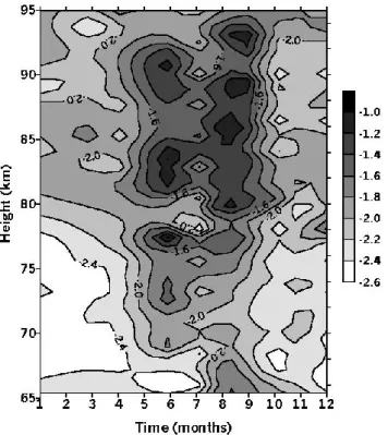
Fig. 3. Height-time section of energy dissipation rates (ε) in the
mesosphere over Gadanki. The contour intervals are .2 W/kg (log
ε).
and shown as error bars in the figure. Similar to the variation of ε with height, Kz also generally increases with increase
in height during the four months of January, April, June and September, as shown in Fig. 2. During the months of January and April, Kzvalues lie in the range of ∼ 10−40 m22 s−1in
the 65–95 km height region, with the larger values occurring at greater heights. The corresponding Kzvalues during June
and September vary in the range of ∼ 25 − 300 m2s−1. In the case of Kz, maximum values are also observed, occurring
during the period from June to September.
The height-time cross section of the turbulent energy dissi-pation rate ε is shown in Fig. 3. It is observed that the turbu-lence intensity is as a maximum during the June to Septem-ber period with lower values occurring during other times. It may be mentioned that the broad maximum in ε values oc-curs during the June to September period, which is the south-west monsoon period over the Indian subcontinent. Similar features are observed for the seasonal variation of Kzas well
(not shown).
If the observed enhancement of ε and Kzduring the June
to September period is associated with the gravity wave ac-tivity, then one may expect a corresponding enhancement in gravity wave activity as well. In order to see any seasonal variation of mesospheric gravity wave activity, M-100 rocket data from 1978 to 1986 at Trivandrum (8.5◦ N, 77◦ E), lo-cated close to Gadanki, were examined. M-100 rockets mea-sured winds and temperatures in the 25–80 km region once a week. The amplitudes of upward propagating gravity waves
Fig. 4. Seasonal variations of proxies for gravity wave activity in
the mesosphere (M-100 rocket data) – See text. (a) Percentage occurrence of temperature lapse rates > 6 K km−1 in the meso-sphere (65–80 km) over Trivandrum (8.5◦N, 77◦E) for a period of 9 years (solid curve), (b) Same as (a) but for Richardson number < 1 (dashed curve).
attain large values at mesospheric heights due to the expo-nential decrease in atmospheric density with an increase in height, and are eventually limited by instabilities and lead to wave breaking, as well as generation of turbulence and wave saturation (e.g. Lindzen, 1981). The instability can be either convective when the wave plus the background state have a negative stability or dynamic when the Richardson number (Ri) has a value less than 0.25. Ideally, one will be able to compute these two parameters from mesospheric tempera-tures and winds, which are measures of instabilities. But the temperature and wind profiles are smoothed (in height), due to limitations in the processing procedures of M-100 rocket data, so that a portion of the vertical variation is essentially removed from the profiles. The smoothing of M-100 rocket data results in very significant attenuation of vertical varia-tion in temperatures and winds with scales less than ∼5 km. In spite of this smoothing, wind and temperature values are given at every km height interval. However, a tendency for the occurrence of instabilities can be computed from these profiles.
Using the M-100 rocket data we have estimated the fre-quency of occurrence of temperature lapse rates (–dT/dz; T is the temperature and z is the height) greater than 6 K km−1 (proxy for convective instabilities), and Ri less than 1 (proxy for shear instability) for every month during 1978–1986 in the 65–80 km height region. The frequency of occurrence is expressed as a percentage of the total number of observed lapse rates and Ri, respectively. This frequency is plotted in Fig. 4 for every month. The actual frequency of occurrence
Fig. 5. A comparison of the energy dissipation rates (ε) in the
meso-sphere over Gadanki with those obtained by others. Thin solid, thin dashed, thick solid and thick dashed lines represent ε over Gadanki for the months of January, April, June and September, respectively. Solid circles and triangles represent ε values reported by Lubken et al. (1993) and Hocking (1990), respectively. Vertical bars show standard errors in ε values over Gadanki in January.
of these two parameters may be much higher than that shown in this figure because of the inherent smoothing of the M-100 data. Both the parameters show minimum during the winter solstice and maxima during the equinoxes. There exists one secondary maximum during summertime for both the param-eters (large lapse rates during July and small Ri during Au-gust). However, it may be noted that secondary maximum during summertime is comparable to the maxima during the equinoxes. If these parameters can be considered as indirect measures of the occurrence of instabilities in the mesosphere, which are presumably the result of very large amplitudes of gravity waves, then their seasonal variation may imply a sim-ilar variation in the gravity wave activity. An earlier study by Hirota (1984) using rocket data had indicated similar semian-nual maxima around the equinoxes for gravity wave activity in the equatorial middle atmospheric region.
The seasonal variation of ε displayed in Fig. 1 and Fig. 3 shows a broad maximum during the months of June to September, whereas that of –dT/dz and Ri, displayed in Fig. 4, shows two equinox maxima and one summer max-imum. Recent observational studies which make use of balloon-measured temperature data show that gravity wave potential energy (Ep) in the stratosphere at low latitudes
(10◦S–20◦S) has a clear annual variation with a maximum during the monsoon months (rainy season) of December to February (Allen and Vincent, 1995). Using temperature pro-files obtained by the GPS/MET experimental data, Tsuda et al. (2000) show that in the 20–30 km height region, Ep is
Fig. 6. A comparison of the eddy diffusion coefficients (Kz) in the
mesosphere over Gadanki with those obtained by others. Solid line represents Kz over Gadanki for the month of December. Dashed
line and solid circles represent winter values of Kz obtained by
R¨ottger (1986) over Arecibo (18.3◦ N, 66◦ W) and Lubken et al. (1993) over high latitudes, respectively. Vertical bars show stan-dard errors in Kzvalues over Gadanki in December.
maximizing during the southern hemispheric summer in the low-latitude regions, such as Indonesian archipelago. Simi-larly, a recent study using a Microwave Limb Sounder (MLS) onboard the Upper Atmosphere Research Satellite (UARS) by McLandress et al. (2000) shows that during the northern hemispheric summer (June to August), gravity wave activ-ity at the ∼38 km level has a maximum lying on and near the Indian subcontinent. McLandress et al. also show that wave activity maxima are correlated with, to a large de-gree, the satellite measurements of outgoing longwave radia-tion, indicating that deep convection is the source of these waves. These studies mentioned above show that strato-spheric gravity wave activity in low latitudes is maximizing during the wet season, implying tropical convection as the source of these waves. Can this strong seasonal variation in the stratospheric gravity wave activity produce a similar sea-sonal variation in the mesosphere? Apparently the summer peak shown in Fig. 4 may correspond to this situation in the mesosphere and one may expect enhanced gravity wave ac-tivity in the mesosphere during summer. It is, therefore, pos-sible that the enhancement of the observed turbulent energy dissipation rate and the vertical eddy diffusion coefficient in the mesosphere over Gadanki is related to the enhanced grav-ity wave activgrav-ity over the low latitude Indian subcontinent during the summer monsoon season (June to September).
It will be interesting to see whether any similar relation-ship between gravity wave activity and turbulence exists at other latitudes as well. A good correspondence between
1024 M. N. Sasi and L. Vijayan: Turbulence characteristics in the tropical mesosphere the gravity wave activity and eddy diffusivity due to
turbu-lence observed by MU radar in the mesosphere over Shi-garaki, Japan (35◦ N, 136◦ E) is reported in the literature.
The observational study by Tsuda et al. (1990) shows that mesospheric gravity wave activity has a semiannual varia-tion with solstice maxima, and Kurosaki et al. (1996) show a very similar seasonal variation for the eddy diffusivity in the mesosphere over Shigaraki with maxima during the solstice periods. These two observations support the hypothesis that turbulence is primarily generated by gravity wave breaking in the mid-latitude mesospheric region. A similar mecha-nism may be operating in the low-latitude mesosphere also, but with a summer (wet season) maximum in gravity wave activity and turbulence parameters.
A comparison has been made between the ε values ob-tained from the present study and the values observed at other geographical locations (Lubken et al., 1993; Hocking, 1990). It is found that ε values over Gadanki during January and April are very close to those at other latitudes, especially at greater heights (Fig. 5). But during the summer season, ε val-ues over Gadanki are much larger when compared to those at higher latitudes below the 80 km height. Yet above 80 km the differences are not significant. Fig. 6 shows a comparison of Kzvalues over Gadanki with those of Lubken et al. (1993)
for a high latitude winter and those of R¨ottger (1986) for a low latitude winter over Arecibo (18.3◦N, 66◦W). The val-ues over Gadanki are shown for the month of December. It is seen that below about the 75 km height, the Kzvalues are
smaller (not very significantly) when compared to those over Arecibo. Above the ∼80 km height, there is hardly any dif-ference between the two sets of Kzvalues. Below ∼75 km,
Kzvalues over Gadanki are larger when compared to those
from Lubken et al. (1993). Above the ∼75 km height the differences between the two are not significant.
4 Summary and conclusions
A method following Hocking (1989) is used to calculate the turbulence parameters from MST radar data in the MLT re-gion. It is found that the turbulence parameters, estimated over Gadanki, show maximum values during the Indian sum-mer monsoon (June to September). The turbulence parame-ters generally show an increase with an increase in height during all seasons. An examination of the seasonal varia-tion of gravity wave activity in the nearby locavaria-tion Trivan-drum shows that gravity wave activity proxies estimated from rocket-measured wind and temperature data have a seasonal variation with equinox and summer maxima. However, re-cent studies of gravity waves using balloon and satellite data show that stratospheric gravity wave activity over low-latitudes maximizes during the wet season in both northern and southern hemispheres. This seasonal variation of gravity wave activity may cause a similar variation in the mesosphere and may be responsible for the observed summer maxima of mesospheric ε and Kz values over Gadanki, resulting from
the gravity wave breakdown leading to enhanced turbulence
generation during the period. The turbulence parameters esti-mated over Gadanki show that above 80 km, their values are not significantly different from those reported for high lati-tudes by in-situ measurements and other low-latitude radar measurements.
Acknowledgements. The National MST Radar Facility (NMRF) is
operated as an autonomous facility under DOS with partial support from CSIR. The authors are very thankful to the scientists and en-gineers from NMRF for making the MST radar observation a suc-cess. Authors gratefully acknowledge many helpful and construc-tive comments by the referees, which helped in the improvement of the manuscript.
Topical Editor J.-P. Duvel thanks two referees for their help in evaluating this paper.
References
Allen, S. J., and Vincent, R. A., Gravity wave activity in the lower atmosphere: Seasonal and latitudinal variations, J. Geophys. Res., 100, 1327–1350, 1995.
Blix, T. A., Thrane, E. V., Fritts, D. C., von Zahn, U., Lubken, F.-J., Hillert, W., Blood, S. P., Mitchell, J. D., Kokin G. A., and Pakhamov, S. V., Small-scale structure observed in-situ during MAC/EPSILON, J. Atmos. Terr. Phys., 52, 835–854,1990. Czechowsky, P. and Ruster, R., VHF radar observations of turbulent
structures in the polar mesopause region, Ann. Geophysicae, 15, 1028–1036, 1997.
CIRA 1986, COSPAR international reference atmosphere: 1986, Part II: Middle atmosphere models, edited by D. Rees, J. J. Bar-nett, and K. Labitzke, pp. 357–381, Pergamon Press, Elmsford, New York, 1990.
Clark, T. E., Hauf, T., and Kuettner, J. P., Convectively forced in-ternal gravity waves: Results from two-dimensional numerical experiments, Quart. J. Roy. Meteorol. Soc, 112, 899–925, 1986. Fritts, D. C., Shear excitation of atmospheric gravity waves, J.
At-mos, Sci., 39, 1936–1952, 1982.
Fritts, D. C., Shear excitation of atmospheric gravity waves, part II: Non-linear radiation from a free shear layer, J. Atmos. Sci., 41, 524–537, 1984.
Fritts, D. C. and Luo, Z., Gravity wave excitation by geostrophic adjustment of the jet stream, Part I: Two-dimensional forcing, J. Atmos. Sci., 49, 681–697, 1992.
Fritts, D. C. and Nastrom, G. D., Sources of mesoscale variability of gravity waves II: Frontal, convective, and jet stream excitation, J. Atmos. Sci., 49, 111–127, 1992.
Fukao, S., Yamanaka, M. D., Ao, N., Hocking, W. K., Sato, T., Yamamoto, M., Nakamura, T., Tsuda, T., and Kato, S., Seasonal variability of vertical eddy diffusivity in the middle atmosphere. 1. Three-year observations by the middle and upper atmosphere radar, J. Geophys. Res., 99, 18973–18987, 1994.
Gage, K. S. and Balsley, B. B., MST radar studies of wind and turbulence in the middle atmosphere, J. Atmos. Terr. Phys., 46, 739–753, 1984.
Hirota, I., Climatology of gravity waves in the middle atmosphere, in Dynamics of the Middle Atmosphere, edited by J. R. Holton, and T. Matsuno, Terra Sientific Publishing Company, Tokyo, Japan, 65–67, 1984.
Hocking, W. K., Measurement of turbulent energy dissipation rates in the middle atmosphere by radar techniques: a review., Radio Sci., 20, 1403–1422, 1985.
Hocking, W. K., Target parameters estimation, MAP Hand Book, 30, 228–268, 1989.
Hocking, W. K., Turbulence in the region 80–120 km., Adv. Space Res., 10 (12), 153–161, 1990.
Hodges, R. R., Generation of turbulence in the upper atmosphere by internal gravity waves, J. Geophys. Res., 72, 3455–3458, 1967. Hodges, R. R., Eddy diffusion coefficients due to instabilities in
internal gravity waves, J. Geophys. Res., 74, 4087–4090, 1969. Kurosaki, S., Yamanaka, M. D., Hashiguchi, H., Sato, T., and
Fukao, S., Vertical eddy difusivity in the lower and middle at-mosphere: a climatology based on the MU radar observations during 1986–1992, J. Atmos. Terr. Phys., 58, 727–734, 1996. Lindzen, R. S., Turbulence and stress owing to gravity waves and
tidal breakdown, J. Geophys. Res., 86, 9707–9714, 1981. Lubken , F.-J., von Zahn, U., Thrane, E. V., Blix, T., Kokin, G.
A., and Pakhomov, S. V., In-situ measurements of turbulent en-ergy dissipation rates and eddy diffussion coefficients during MAP/WINE, J. Atmos. Terr. Phys., 49, 763–775, 1987. Lubken, F.-J., Hillert, W., Lehmacher, G., and von Zahn, U.,
Ex-periments revealing small impact of turbulence on the energy revealing small impact of turbulence on the energy budget of the mesosphere and lower thermosphere, J. Geophys. Res., 98, 20369–20384, 1993.
McIntyre, M. E., On dynamics and transport near the polar mesopause in summer, J. Geophys. Res., 94, 14617–14628, 1989.
McLandress, C., Alexander, M. J., and Wu, D. L., Microwave Limb Sounder observations of gravity waves in the stratosphere: A climatology and interpretation , J. Geophys. Res., 105, 11947–
11967, 2000.
Nastrom, G. D. and Fritts, D. C., Sources of mesoscale variability of gravity waves, I: Topographic excitation, J. Atmos. Sci., 49, 101–110, 1992.
Nastrom, G. D., Fritts, D. C., and Gage, K. S., An investigation of terrain effects on the mesoscale spectrum of atmospheric mo-tions, J. Atmos. Sci., 44, 3087–3096, 1987.
Rao, P. B., Jain, A. R., Kishore, P., Balamuralidhar, P., Damle, S. H., and Viswanathan, G., Indian MST radar 1, system description and sample vector wind measurements in ST mode, Radio Sci., 30, 1125–1138, 1995.
R¨ottger, J., The use of experimentally deduced Brunt-Vaisala fre-quency and turbulent velocity fluctuations to estimate the eddy diffusion coefficient, MAP Handbook, 20, 173–178, 1986. Sasi, M. N. and Sengupta, K. , A reference atmosphere for Indian
equatorial zone from surface to 80 km–1985, Scientific report SPL: SR:006:85, Space Physics Laboratory, Vikram Sarabhai Space Centre, Trivandrum, India, 1986.
Tsuda, T., Murayama, Y., Yamamoto, M., Kato, S., and Fukao, S., Seasonal variations of momentum flux in the mesosphere ob-served with the MU radar, Geophys. Res. Lett., 17, 725–728, 1990.
Tsuda, T., Nishida, M., Rocken, C., and Ware, R. H., A global cli-matology of gravity wave activity in the stratosphere revealed by the GPS occultation data (GPS/MET), J. Geophys. Res., 105, 7257–7273, 2000.
Weinstock, J., Vertical turbulent diffusion in a stably stratified fluid, J. Atmos. Sci., 35, 1022–1027, 1978.