Multivariate linear parametric models applied to daily rainfall time series

(1)

HAL Id: hal-00296844

https://hal.archives-ouvertes.fr/hal-00296844

Submitted on 31 Mar 2005

HAL is a multi-disciplinary open access

archive for the deposit and dissemination of

sci-entific research documents, whether they are

pub-lished or not. The documents may come from

teaching and research institutions in France or

abroad, or from public or private research centers.

L’archive ouverte pluridisciplinaire HAL, est

destinée au dépôt et à la diffusion de documents

scientifiques de niveau recherche, publiés ou non,

émanant des établissements d’enseignement et de

recherche français ou étrangers, des laboratoires

publics ou privés.

Multivariate linear parametric models applied to daily

rainfall time series

S. Grimaldi, F. Serinaldi, C. Tallerini

To cite this version:

S. Grimaldi, F. Serinaldi, C. Tallerini. Multivariate linear parametric models applied to daily rainfall

time series. Advances in Geosciences, European Geosciences Union, 2005, 2, pp.87-92. �hal-00296844�

(2)

Advances in Geosciences, 2, 87–92, 2005 SRef-ID: 1680-7359/adgeo/2005-2-87 European Geosciences Union

Advances in

Geosciences

Multivariate linear parametric models applied to daily rainfall time

series

S. Grimaldi1, F. Serinaldi2, and C. Tallerini2

1_{Institute of Research for Hydrogeological Protection, CNR-IRPI, Perugia Italy}

2_{Department of Hydraulics, Transportations and Highways, University of Rome “La Sapienza”, Rome, Italy}

Received: 18 November 2004 – Revised: 15 February 2005 – Accepted: 4 March 2005 – Published: 31 March 2005

Abstract. The aim of this paper is to test the

Multivari-ate Linear Parametric Models applied to daily rainfall series. These simple models allow to generate synthetic series pre-serving both the time correlation (autocorrelation) and the space correlation (crosscorrelation). To have synthetic daily series, in such a way realistic and usable, it is necessary the application of a corrective procedure, removing negative values and enforcing the no-rain probability. The following study compares some linear models each other and points out the roles of autoregressive (AR) and moving average (MA) components as well as parameter orders and mixed parame-ters.

1 Introduction

Daily synthetic series are used in several hydrological appli-cations. In many cases the univariate analysis is not enough, since rainfall series are affected by strong space correla-tion and a weak time correlacorrela-tion as well. Therefore in a rainfall-scenario simulation the multivariate approach is nec-essary. In this paper, Multivariate Linear Parametric Models (MLPM) are applied as an extension of the well known Lin-ear Parametric Models (LPM) (Grimaldi, 2004).

Rainfall series are particularly difficult to model with a LPM. Usually they are not perfectly linear, non-Gaussian, and present weak seasonality and a high percentage of zero values (no-rain days). Despite those limits, simulations ob-tained with LPM preserve the main statistical characteristics of the observed series (Grimaldi et al., 2004). The main prob-lem is the presence of negative values in the synthetic series, an obvious consequence of stochastic nature of these pro-cesses that cannot reproduce a sequence of zero-values. In order to overcome this limit we referred to the corrective pro-cedure, already applied in Grimaldi et al. (2004), on 20 daily rainfall series.

Correspondence to: S. Grimaldi (salvatore.grimaldi@irpi.cnr.it)

Here follows comparisons among MLPMs. The purpose is to point out differences among simple and widely used first-order Vector Autoregressive models, optimal-order Vec-tor AuVec-toregressive models and general VecVec-tor AuVec-toregressive Moving Average models described in Sect. 2. The present case study, Sect. 3, also examines the possibility to reduce the number of the parameters in the modelling.

2 Multivariate linear parametric models

A multivariate stochastic process can be described by vari-ables characterized by the autocorrelation, in time domain, and the crosscorrelation in the space-time domain. As in the univariate case, these correlations can be expressed by means of parameter linear combinations. The general class of multivariate linear parametric model is called VARMA(p,q) (Vector Autoregressive Moving Average, Hall and Nicholls, 1979; Lutkepohl, 1993; Hipel and McLeod, 1994):

yt =ν + A1yt −1+A2yt −2+... +Apyt −p+ut

+M1ut −1+M2ut −2+... +Mqut −q (1)

where yt= {y1t, y2t, ..., ykt}is k-dimension vector of vari-ables at the time t , ν= {ν1, ν2, ..., νk}is a constant vector,

ut= {u1t, u2t, ..., ukt}white-noise vector, and where

Ai = ai11ai12...ai1k ai21ai22...ai2k ... aik1aik2...aikk i =1, 2, ..., p, Mi = mi11mi12...mi1k mi21mi22...mi2k ... mik1mik2...mikk i =1, 2, ..., q,

are respectively the Autoregressive and the Moving average coefficient matrices. Since this general expression is usually characterized by a high number of parameters and a complex

(3)

88 S. Grimaldi et al.: Multivariate linear parametric models 15 85 155 225 295 365 Days -2 02468 Mean ( mm) Classic method STL method 15 85 155 225 295 365 Lag 0 5 10 15 20 Standar d de viation ( mm)

Figure 1. Seasonal components of series 1 with classic method and STL method applied with

smoothing windows of 175 lags.

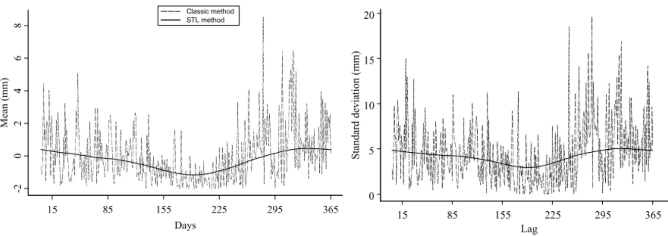
Fig. 1. Seasonal components of series 1 with classic method and STL method applied with smoothing windows of 175 lags.

0 200 400 600 800 1000 1200 Lag 0. 0 0. 2 0. 4 0. 6 0. 8 1. 0 A C F Se rie s 1 0 2 4 6 8 10 0. 0 0. 2 0. 4 0. 6 0. 8 1. 0 0 200 400 600 800 1000 1200 Lag 0. 00 .2 0. 40 .6 0. 81 .0 C C F Ser ies 1 -2 0 2 4 6 8 10 0. 0 0.2 0. 4 0.6 0. 8 1. 0

- In the line 23 on the left of page 3 remove (Grimaldi, in rewiew)

- In the line 4 on the right of page 3 “….. and the crosscorrelation functions “ substitute “the”

with “a”

- In References, the correct year is 1979.

Fig. 2. Autocorrelation Function of series 1 (a) and Cross Correlation Function of series 1–2 (b). The small graph reproduces the above functions until 10 lags.

parameter estimation procedure, in literature it is often sim-plified. The most used expression is the VAR(p) easy to be built, which develops only the AR component. Sometimes, even only the first order is considered, VAR(1). Another sim-plified version is the Contemporaneous ARMA(p,q) models (CARMA, Hypel and McLeod, 1994), where all the mixed parameters of both matrices A and M are fixed to zero. This means that the model can preserve the full autocorrelation, but the crosscorrelation only at lag 0; so rainfall simulation will reproduce only the contemporaneous space correlation.

The procedure to build an MLPM is the same as the uni-variate case (Grimaldi, 2004). It consists of 4 steps (Prelimi-nary Analysis, Parameter estimation, Checking and Optimal model choice, Simulation) useful to identify the best model analysing the observed data and generate synthetic scenarios. The Preliminary analysis tests the Gaussianity and stationar-ity on the series. In the first case the Box and Cox transfor-mations are applied, but this approach could prove to be not useful to daily rainfall modelling (Grimaldi, 2004). Concern-ing the Stationarity, the seasonal characteristics are analysed. The Deseasonalization of single series can be performed

fil-tering series yit with the expression

zτ_it =y

τ it−µiτ

siτ

i =1, 2, ..., k. (2) The classic mean (µiτ)and the standard deviation (siτ) periodical components are smoothed using the STL method (Seasonal trend decomposition based on Loess, Grimaldi, 2004). As shown in Fig. 1 this approach is necessary to remove the high noise due to the daily series scale. In daily rainfall series the seasonality could be not significant (Grimaldi et al., 2004, Grimaldi et al., 2004). The Parameter Estimation step uses several methods, such as Yule-Walker (Whittle, 1963), Burg algorithm (Trinidade et al., 2002), OLS (Ordinary Least Square, Lutkepohl, 1993), and MLE (Maximun Likehood Estimation, Shea 1989; Lutkephol, 1993). The following case study uses Lutkephol’s (Approx-imate) MLE method. Together with OLS estimation, there are also methods to reduce the number of the parameters to be estimated, and obtain the so-called Subset VAR models (Lutkephol, 1993). The Checking and Optimal model choice step must check that, for all estimated models, all the residual series are white noises . This is possible through Portmanteau

(4)

S. Grimaldi et al.: Multivariate linear parametric models 89

(a)

1 2 Series3 4 5 50 100 150 200 250 300 350 400 R ainf all ( m m ) 50 Simulated Series Observed

(b)

1 2 Series3 4 5 50 10 0 150 200 250 300 350 40 0 Ra in fa ll ( m m) 50 Simulated Series Observed

Figure 3. Maximum values of the observed series and of the 50 simulated series. The box-plot

represents the mean of the maximum values and the 5% and 95% quantiles estimated on

the 50 synthetic values. The results are obtained: a) without the deseasonalization

procedure b) with the deseasonalization procedure.

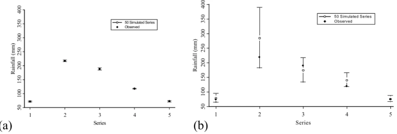
Fig. 3. Maximum values of the observed series and of the 50 simulated series. The box-plot represents the mean of the maximum values and the 5% and 95% quantiles estimated on the 50 synthetic values. The results are obtained: (a) without the deseasonalization procedure (b) with the deseasonalization procedure.

Test (Hosking, 1980). Among models positive to this test, the best one is selected by Automatic Selection Index like AIC (Akaike Information Criterion) or SBC (Schwartz Bayesian Criterion). The last step, Simulation, allows to generate syn-thetic series starting from the selected optimal model. The used simulation algorithm is explained in Lutkepohl (1993) and, as in the univariate case (Grimaldi, 2004), the genera-tion of innovagenera-tions is carried out by re-sampling the residu-als obtained from the observed series. The multivariate case develops a vectorial sampling, so that the contemporaneous correlation is preserved.

As introduced in Sect. 1, these models create negative val-ues in synthetic series, despite their capability to reproduce the main statistics of the observed series. In order to over-come this difficulty, the above-mentioned corrective proce-dure is necessary. Briefly, this proceproce-dure consists in: (i) transferring the abscissa until the negative-value frequency of the simulated series is equal to the no-rain frequency, (ii) changing the negative values in zero-values; (iii) increasing rainy-days values so that enforcing the mean of the observed series. This procedure does not modify the positive tail of the distribution and make the synthetic series realistic and usable.

3 The case study

The present case study analyses five daily rainfall series from 1958 to 1979 (Rudari, 2001) observed in some stations of Tuscany, a region of Italy . The examined series originally were lacking in some values and years. The case-study sam-ple is obtained removing the years without values, interpo-lating missing values and removing 29 February. The final sample consists of a lap of 15 years. Figure 2 shows the au-tocorrelation (ACF) and a crosscorrelation functions (CCF) of one of the series. As expected there is a weak time cor-relation and a significant space corcor-relation as well as a very weak seasonal state.

On the 5 described series the following tests are devel-oped:

1. A comparison between the modelling with the desea-sonalization procedure (smoothing window=175) and the modelling without it.

2. A comparison among different models: Var(1), the sim-plest and the most used, the optimal Var(p) and the op-timal mixed Varma(p,q)

3. A comparison between models with different number of parameters: Complete Var(p) and Subset Var(p) with the lowest possible number of parameters.

The evaluations were carried out comparing 5 groups of 50 synthetic series, simulated with the different models or pro-cedures, to those observed ones.

Applying on the 5 series the procedure briefly described in Sect. 2, both AIC and SBC index suggest Var(2) as opti-mal model among Vector AR models, and Varma(1,1) among Vector ARMA models, in particular Portmanteau Test is per-formed with maximum lag=20 and 5% significant level.

Firstly the test (a) is approached. The seasonal compo-nents of considered series are very weak (see Figs. 1 and 2) and in fact, looking at the ACF (Fig. 2), the sinusoid with period 365 is almost within the 95% confidence bounds. Fig-ure 3 compares maximum values of the simulated series with and without the application of the deseasonalization proce-dure and the observed maximum values. It without signifi-cant seasonality, the inversion of filter (2) increase the vari-ance of simulated series.

(5)

90 S. Grimaldi et al.: Multivariate linear parametric models

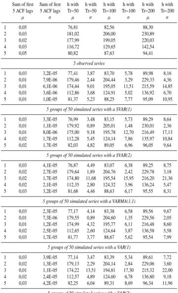
Table 1a. Statistical parameters estimated on observed and 50 sim-ulated series.

mean mean variance variance skewness skewness max value max value

µ σ µ σ µ σ µ σ 1 2,00 33,51 4,70 72,00 2 1,86 41,45 10,54 217,00 3 2,84 68,49 6,27 187,90 4 2,42 42,05 5,01 117,80 5 2,38 37,56 4,26 72,60 5 observed series 1 2,00 0,00 30,93 0,03 4,78 0,00 72,02 1,55 2 1,86 0,00 38,72 0,02 11,20 0,01 217,09 1,60 3 2,84 0,00 64,58 0,07 6,56 0,00 187,88 0,78 4 2,42 0,00 39,75 0,04 5,18 0,00 117,67 0,51 5 2,38 0,00 34,47 0,03 4,37 0,00 72,65 0,79

5 groups of 50 simulated series with a SVAR(1)

1 2,00 0,00 30,57 0,03 4,81 0,00 72,17 1,45

2 1,86 0,00 38,71 0,02 11,19 0,01 216,90 1,09

3 2,84 0,00 64,19 0,10 6,61 0,00 187,92 2,01

4 2,42 0,00 39,43 0,03 5,22 0,00 117,83 0,88

5 2,38 0,00 34,13 0,04 4,39 0,00 72,60 0,87

1 2,00 0,00 30,07 0,09 4,85 0,00 71,76 1,43

2 1,86 0,00 38,46 0,06 11,29 0,01 217,25 2,67

3 2,84 0,00 63,82 0,07 6,65 0,00 188,19 5,34

4 2,42 0,00 38,90 0,04 5,26 0,00 117,71 0,61

5 2,38 0,00 33,61 0,07 4,42 0,00 72,72 2,27

5 groups of 50 simulated series with a VARMA(1,1)

1 2,00 0,00 30,42 0,03 4,82 0,00 71,82 0,64

2 1,86 0,00 38,51 0,04 11,23 0,00 216,78 0,65

3 2,84 0,00 63,90 0,07 6,62 0,00 188,02 2,44

4 2,42 0,00 39,12 0,04 5,23 0,00 117,74 0,77

5 2,38 0,00 33,91 0,03 4,40 0,00 72,85 1,81

5 groups of 50 simulated series with a VAR(1)

1 2,00 0,00 30,19 0,04 4,84 0,00 72,28 2,23

2 1,86 0,00 38,45 0,04 11,25 0,01 216,89 1,34

3 2,84 0,00 63,74 0,10 6,64 0,00 187,69 2,03

4 2,42 0,00 39,05 0,04 5,25 0,00 117,98 1,69

5 2,38 0,00 33,79 0,05 4,44 0,00 73,48 5,13

In order to compare the simulated and the observed se-ries in the tests (a) and (b) the following parameters are mainly investigated: mean, variance, skewness, maximum values, the sum of the first 5 steps of the ACF, rainfall with 50-, 100-, 200-year return time (defined by standard extreme value analysis using Gumbel distribution), wet-dry period transition frequency (frequency of n consecutive rainy days, followed and preceded by dry days), distributions on cumula-tive rainfall of events of length n-days, crosscorrelation func-tion.

Usually the model used in literature is the Var(1). In this study the optimal model improvements are tested (Var(2) and Varma(1,1)) without deseasonalization procedure. The Ta-ble 1 compares the above-described statistical parameters , estimated on the observed series and the 50 simulated ones, Fig. 4 shows an example of comparison between CCF of the simulated series and the observed series functions, that is characteristic for all the simulated series; Fig. 5 shows the

Table 1b. Statistical parameters estimated on observed and 50 sim-ulated series.

Sum of first Sum of first h with h with h with h with h with h with

5 ACF lags 5 ACF lags Tr=50 Tr=50 Tr=100 Tr=100 Tr=200 Tr=200

µ σ µ σ µ σ µ σ 1 0,05 76,81 82,56 88,30 2 0,03 181,02 206,00 230,89 3 0,02 177,99 199,05 220,03 4 0,03 116,72 129,65 142,54 5 0,05 80,82 87,63 94,41 5 observed series 1 0,03 3,2E-05 77,41 3,87 83,70 5,78 89,98 8,16 2 0,01 7,9E-06 179,46 2,44 204,44 3,29 229,33 4,36 3 0,01 6,1E-06 174,44 9,01 195,05 11,51 215,59 14,85 4 0,01 3,6E-06 112,86 3,68 124,91 5,02 136,92 6,70 5 0,01 1,0E-05 81,37 5,23 88,25 7,77 95,09 10,95

1 0,03 3,3E-05 76,99 3,48 83,15 5,73 89,29 8,64

2 0,01 1,1E-05 179,92 0,89 205,01 1,48 230,01 2,36

3 0,01 8,0E-06 175,00 9,18 195,78 12,70 216,49 17,13

4 0,02 1,7E-05 112,28 5,45 124,14 7,86 135,97 10,84

5 0,02 1,7E-05 82,03 4,82 89,05 6,96 96,05 9,64

1 0,03 4,1E-05 76,87 4,49 83,07 6,38 89,25 8,75

2 0,02 2,7E-05 179,64 1,89 204,76 2,42 229,78 3,18

3 0,02 1,7E-05 174,80 11,68 195,54 15,95 216,20 21,36

4 0,02 2,1E-05 112,35 2,80 124,32 3,96 136,24 5,47

5 0,03 3,2E-05 81,68 4,46 88,63 6,17 95,55 8,31

5 groups of 50 simulated series with a VARMA(1,1)

1 0,03 2,3E-05 77,17 4,14 83,38 6,58 89,56 9,67

2 0,01 7,3E-06 179,55 0,89 204,60 1,35 229,56 2,05

3 0,01 1,2E-05 174,99 4,32 195,77 6,11 216,48 8,60

4 0,02 2,5E-05 112,65 2,60 124,64 3,87 136,58 5,58

5 0,03 1,7E-05 81,77 3,77 88,67 5,62 95,54 7,99

1 0,03 3,9E-05 77,14 3,47 83,39 5,34 89,61 7,72

2 0,02 1,3E-05 179,13 2,29 204,14 2,84 229,06 3,60

3 0,01 1,1E-05 174,22 13,51 194,81 17,30 215,32 22,00

4 0,02 2,4E-05 112,57 4,89 124,60 6,78 136,60 9,18

5 0,03 4,2E-05 82,25 6,04 89,31 8,69 96,34 11,96

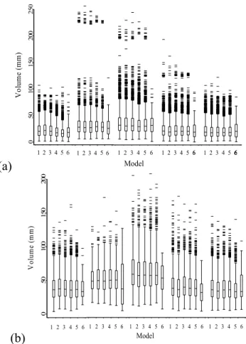
transition frequency and Fig. 6 shows the 5- and 3-days cu-mulative rainfall events. Observing the results it is possible to note that the optimal models provide more accurate results above all those concerning the crosscorrelation values.

Another purpose of this study case regards the number of parameters. The Vector Ar(p) model is characterized by

p×n2 parameters, for instance a simple Var(2) applied on 5 series needs 50 parameters. To overcome this limit they can be reduced by fixing no-significant parameters to zero. Following the T-ratio approach, a SVar(1) with 6 parame-ters and a SVar(2) with 14 parameparame-ters are defined and then estimated with EGLS method (Lutkepohl, 1993). Looking at the obtained results in Table 1, Figs. 4, 5 and 6 it is ev-ident that these simple models statistically lose information but also that they are able to generate usable daily rainfall synthetic series.

(6)

S. Grimaldi et al.: Multivariate linear parametric models 91 Matrix element 1 7 13 19 25 0.3 0.4 0.5 0.6 0.7 0.8 0.9 1.0 C ro ss C or re la tio n V alu es Matrix element 26 32 38 44 50 0.06 0.11 0.16 0.21 Varma(1,1) Var(1) Obeserved SVar(1) Var(2) SVar(2) Matrix element 51 57 63 69 75 0.00 0.03 0.06 0.09 C ross C or re la tion V alue s Matrix element 76 82 88 94 100 0.00 0.02 0.04 0.06 0.08

Figure 4. Crosscorrelation-matrix representation related to Var(1), Var(2), SVar(1), SVar(2),

Varma(1,1). Boxes show: (a) 25 values of crosscorrelation matrix at lag = 0; (b) 25 values

of crosscorrelation matrix at lag = 1 (c) 25 values of crosscorrelation matrix at lag = 2 (d)

25 values of crosscorrelation matrix at lag = 3.

Fig. 4. Crosscorrelation-matrix representation related to Var(1), Var(2), SVar(1), SVar(2), Varma(1,1). Boxes show: (a) 25 values of crosscorrelation matrix at lag=0; (b) 25 values of crosscorrelation matrix at lag=1 (c) 25 values of crosscorrelation matrix at lag=2 (d) 25 values of crosscorrelation matrix at lag=3.

4 Conclusion

In this paper the multivariate linear parametric modelling is applied on 5 daily rainfall time series. The first aim of the application is to test this approach then examine the differ-ences among several models like: Var(1), optimal Var(p) and Varma(p,q). The described case study shows that this mod-elling can simulate rainfall time series and that the optimal models prove to be favourable instead of the simplest Var(1). The limit of these models is the number of the parameters. It frequently happens to have cases with 50 or 70 parameters to estimate. The case study highlights that the Subset Var models can reduce the number of the parameters keeping the results good for hydrological application.

Series 1 Series 2 Series 3 Series 4 Series 5

0 75 15 0 22 5 300 37 5 45 0 1 2 3 4 5 1 2 3 4 5 1 2 3 4 5 1 2 3 4 5 1 2 3 4 5 1 2 3 4 5 _Model Transit io n fr eq uency

Figure 5, Transition Frequency of 5 days estimated on each of the observed series (black point) and on the 50 simulated series using a Var(1) [1], SVar(1) [2] , SVar(2) [3], Var(2)

[4], Varma(1,1) [5]

Fig. 5. Transition Frequency of 5 days estimated on each of the observed series (black point) and on the 50 simulated series using a Var(1) [1], SVar(1) [2] , SVar(2) [3], Var(2) [4], Varma(1,1) [5].

(7)

92 S. Grimaldi et al.: Multivariate linear parametric models

(a)

V ol ume ( m m) Model 0 50 100 150 20 0 250 6 5 4 3 2 1 1 2 3 4 5 6 1 2 3 4 5 6 1234566 123456666

(b)

Vo lu m e ( m m ) Model 0 50 100 150 20 0 1 2 3 4 5 6 1 2 3 4 5 6 1 2 3 4 5 6 1 2 3 4 5 6 1 2 3 4 5 6

Figure 6. Volume box plots of 3- (a) and 5- (b) days events. Each block of six box-plots is

referred to a series. The box-plots 1,2,3,4 and 5 are referred to the 50 simulated series

obtained with Var(1) [1], SVar(1) [2] , SVar(2) [3], Var(2) [4], Varma(1,1) [5].

The box plot 6 is referred to the observed series. The box-plots are characterized by the

median, the 25% and 75% interquartile and the outliers.

Fig. 6. Volume box plots of 3- (a) and 5- (b) days events. Each block of six box-plots is referred to a series. The box-plots 1,2,3,4 and 5 are referred to the 50 simulated series obtained with Var(1) [1], SVar(1) [2] , SVar(2) [3], Var(2) [4], Varma(1,1) [5]. The box plot 6 is referred to the observed series. The box-plots are character-ized by the median, the 25% and 75% interquartile and the outliers.

Acknowledgements. The authors thanks R. Rudari for rainfall data

and for precious comments on obtained results. This work was supported by CNR-GNDCI.

Edited by: L. Ferraris

Reviewed by: A. Cancelliere and other referees

References

Box, G. E. P. and Cox, D.: An analysis of transformation (with discussion), Journal of the Royal Statistical Society, B, 26, 211– 246, 1964.

Grimaldi, S.: Linear parametric models applied on daily hydrolog-ical series, Journal of Hydrologic Engineering, 9, 5, 383–391, 2004.

Grimaldi, S., Tallerini, C., and Serinaldi, F.: “Modelli multivariati lineari per la generazione di serie di precipitazioni giornaliere”, Proceedings, Giornata di Studio: Metodi Statistici e Matematici per l’Analisi delle Serie Idrologiche, Napoli, maggio 2004. Hipel, K. W. and McLeod, A. I.: Time Series Modelling of Water

Resources and Environmental Systems, Elsevier Science, 1994. Hosking, J. R. M.: The Multivariate Portmanteau Statistic, Journal

of the American Statistical Association, 75, 371, 502–608, 1980. Hall, A. D. and Nicholls, D. F.: The Exact Maximum Likelihood Function of Multivariate Autoregressive Moving Average Mod-els, Biometrika, 66, 259–264, 1979.

Lutkepohl, H.: Introduction to Multiple Time Series Analysis, 2nd Edition, Springer-Verlag, Berlin, 1993.

Rudari, R.: Predicibilit`a del clima europeo ed influenze delle forzanti a scala sinottica su eventi regionali di precipitazione in-tensa”, PhD Thesis, manuscript in Italian, 2001.

Shea, B. L.: The exact likelihood of a Vector Autoregressive Mov-ing Average model, Applied Statistics, 38(1), 161–184, 1989. Trindade, A., Brockwell, P. J., and Dahlhaus, R.: Modified Burg

Al-gorithms for Multivariate Subset Autoregression, Technical Re-port 2002-015, Department of Statistics, University of Florida, 2002.

Whille, P.: On the fitting of multivariate autoregressions, and the approximate canonical factorization of spectral density matrix, Biometrika, 50, 1/2, 129–134, 1963.