Equatorial ionospheric zonal drift model and vertical drift statistics from UHF scintillation measurements in South America

(1)

HAL Id: hal-00317637

https://hal.archives-ouvertes.fr/hal-00317637

Submitted on 23 Sep 2004

HAL is a multi-disciplinary open access

archive for the deposit and dissemination of

sci-entific research documents, whether they are

pub-lished or not. The documents may come from

teaching and research institutions in France or

abroad, or from public or private research centers.

L’archive ouverte pluridisciplinaire HAL, est

destinée au dépôt et à la diffusion de documents

scientifiques de niveau recherche, publiés ou non,

émanant des établissements d’enseignement et de

recherche français ou étrangers, des laboratoires

publics ou privés.

drift statistics from UHF scintillation measurements in

South America

R. E. Sheehan, C. E. Valladares

To cite this version:

R. E. Sheehan, C. E. Valladares. Equatorial ionospheric zonal drift model and vertical drift statistics

from UHF scintillation measurements in South America. Annales Geophysicae, European Geosciences

Union, 2004, 22 (9), pp.3177-3193. �hal-00317637�

(2)

SRef-ID: 1432-0576/ag/2004-22-3177 © European Geosciences Union 2004

Annales

Geophysicae

Equatorial ionospheric zonal drift model and vertical drift statistics

from UHF scintillation measurements in South America

R. E. Sheehan and C. E. Valladares

Institute for Scientific Research, Boston College, Chestnut Hill, Massachusetts, USA

Received: 17 December 2003 – Revised: 8 April 2004 – Accepted: 14 May 2004 – Published: 23 September 2004 Part of Special Issue “Equatorial and low latitude aeronomy”

Abstract. UHF scintillation measurements of zonal

iono-spheric drifts have been conducted at Ancon, Peru since 1994 using antennas spaced in the magnetic east-west direction to cross-correlate geo-synchronous satellite signals. An em-pirical model of average drift over a wide range of Kp and

solar flux conditions was constructed from successive two-dimensional fits of drift vs. the parameters and day of year. The model exhibits the typical local time trend of maximum eastward velocity in the early evening with a gradual de-crease and reversal in the early morning hours. As expected, velocities at all hours increase with the solar flux and de-crease with Kpactivity. It was also found that vertical drifts

could contribute to the variability of drift measurements to the east of Ancon at a low elevation angle. The vertical drift at the ionospheric intersection to the east can be estimated when combined with nearly overhead observations at An-con or a similar spaced-antenna site at Antofagasta, Chile. Comparisons on five days with nearly simultaneous mea-surements of vertical drift by the Julia radar at Jicamarca, Peru show varying agreement with the spaced-antenna esti-mates. Statistical results from 1997 to 2001 generally agree with radar and satellite studies.

Key words. Ionosphere (equatorial ionosphere; ionospheric

irregularities; modeling and forecasting)

1 Introduction

A comprehensive understanding of the low latitude plasma electrodynamics is of great importance because of the con-trolling influence that plasma drifts and thermospheric winds exert on the number density distribution and on developing the favorable states conducive to the initiation of large-scale plasma bubbles. In general, the neutrals transfer momentum to the ions by collisions. In the F-region the ions move almost freely along the field lines; similarly, they create polariza-Correspondence to: R. E. Sheehan

(sheehanp@bc.edu)

tion electric fields that transport the plasma perpendicular to the B-field. During quiet magnetic conditions, the E- and F-region neutral wind dynamos generate the equatorial electric fields (Rishbeth, 1970, 1981; Eccles, 1998). During mag-netically disturbed periods, the penetration of E-field from high latitudes and the ionospheric disturbed dynamo can sig-nificantly modify the magnitude of the low latitude electric fields (Fejer and Scherliess, 1997).

At low latitudes the climatology of the zonal and verti-cal drifts has been defined based on measurements collected with incoherent scatter radars, satellites and scintillation re-ceivers. Fejer et al. (1981, 1985) used measurements of drifts performed at Jicamarca to show that the zonal drift is west-ward and about 50 m/s during the day, and eastwest-ward and up to 130 m/s during the night. Coley and Heelis (1989) used drifts collected with the DE-2 satellite to show that these drifts coincided with the Jicamarca drifts. Their evening val-ues of zonal eastward drifts peaking at 170 m/s were typical for solar maximum conditions. They also observed drift re-versals from westward to eastward at 19:00 LT and to west-ward drifts at 04:30 LT. Recently, Fejer and Scherliess (1998) were able to extract the temporal evolution of the low latitude penetration zonal drifts that is driven by the magnetospheric E-field. They observed the largest effect on the dusk to mid-night sector with an average duration of 2 h. Valladares et al. (1996) presented irregularity drifts observed during the first year of operations at Ancon. Their values were in agree-ment with the values measured at Jicamarca for solar mini-mum conditions.

More recently, Valladares et al. (2002) have compared the zonal drift measured with the scintillation technique at An-con and the zonal wind measured by the FPI located at Are-quipa. The drifts were close to the wind values;, with the drifts exceeding the winds by 15 m/s during the equinox and the opposite behavior was seen during the June solstice. They attributed the larger drift values to spatial variability of the zonal wind.

This paper presents statistical results of the zonal drifts measured using the spaced-antenna scintillation technique at

(3)

90 80 70 60-40 -30 -20 -10 0 10 F7 F8 F7 F8

Geographic Longitude (West)

Geographic Latitude Ionospheric Intersections Magnetic Equator 15 deg. magnetic latitude 15 deg. magnetic latitude Ancon Jicamarca Antofagasta

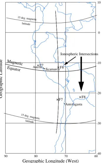
Fig. 1. Map of the west coast of South America showing the spaced-receiver sites at Ancon, Peru and Antofagasta, Chile, and the Julia radar at Jicamarca, Peru. F7 and F8 near Ancon indicate the 350-km ionospheric intersections of the Ancon-W and Ancon-E ray paths, respectively, to the F7 and F8 geostationary satellites. F7 and F8 near Antofagasta are the intersection points from Antofagasta to the same satellites.

two sites located near the west coast of South America. One of the sites, Ancon, Peru, is located near the magnetic equa-tor, and the other is at Antofagasta, Chile (11◦S magnetic lat-itude, 5◦east of Ancon). The study constitutes a continuing effort to develop an empirical model of the climatology and day-to-day variability of the zonal irregularity drift as a func-tion of local time, season, magnetic, and solar condifunc-tions. It also seeks to represent the spatial and altitude/latitude depen-dency of the zonal drifts during the nighttime hours.

In a related effort, spaced receiver measurements at Ancon from a low-elevation satellite to the east were combined with Antofagasta drifts to give estimates of vertical drift velocities near Antofagasta. The vertical drift is an important factor in the instability leading to equatorial spread F and plasma bubbles (Fejer et al., 1999). Several case studies compare the results with data from the Julia radar at Jicamarca.

2 Experimental setup

The spaced receiver system at Ancon described in Valladares et al. (1996) cross-correlates UHF signal level data at 50 Hz from two geo-synchronous satellites, one nearly overhead lo-cated at 100◦_{west longitude (F7), the other low to the east}

at 23◦west longitude (F8). Figure 1 shows the locations of Ancon and a similar spaced antenna system at Antofagasta, Chile, along with the 350-km ionospheric intersection points along the ray paths to the satellites. The intersection points F7 and F8 near Ancon will be designated W, Ancon-E, respectively. Similarly, the points F7 and F8 near Antofa-gasta are the corresponding ionospheric intersections from Antofagasta. With the addition of Ancon-E in 1996, S4 and drift data have been collected nearly continuously up to the present.

Drift velocities at Ancon are calculated on-line using methods from Vacchione et al. (1987). This method uses quadratic approximations near the peaks of the cross- and autocorrelation functions to estimate both the drift veloc-ity, V0, and the random velocity, Vc, which is related to

the amount of decorrelation over the sample time interval. When Vc=0 (maximum cross-correlation=1), V0is identical

to the apparent drift velocity calculated from the lag of the maximum cross-correlation. V0decreases relative to the

ap-parent velocity as Vc increases (maximum cross-correlation

decreases).

3 Statistical results

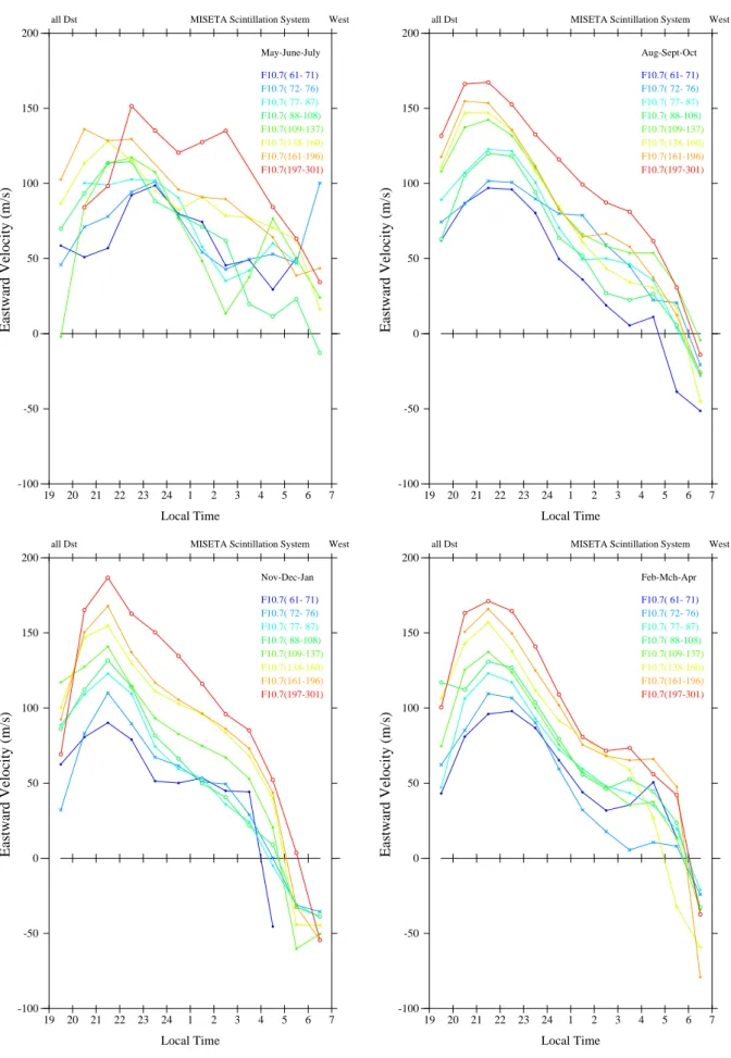
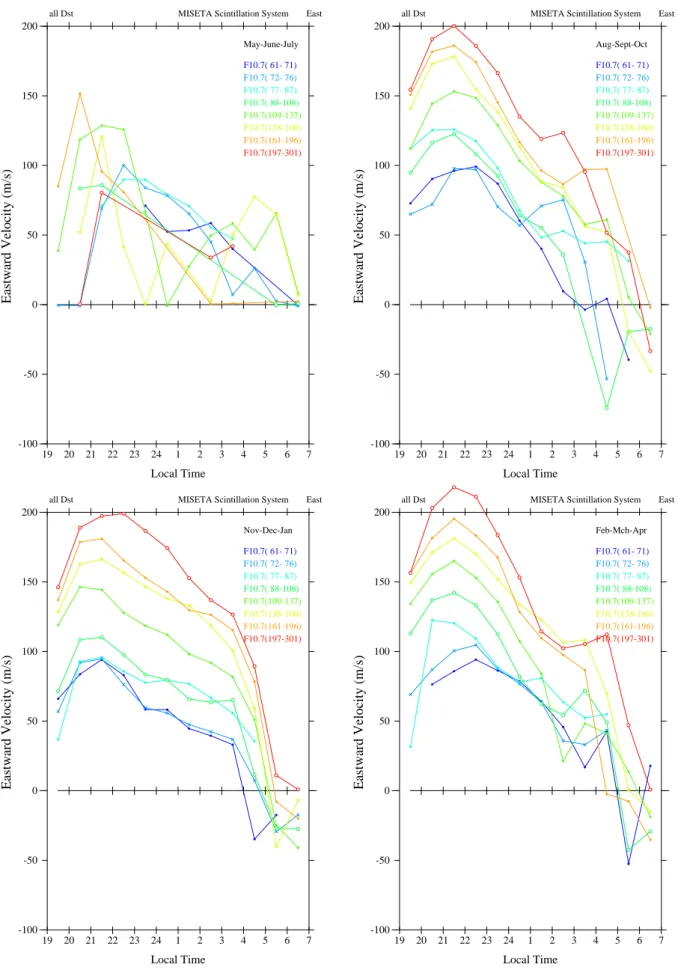
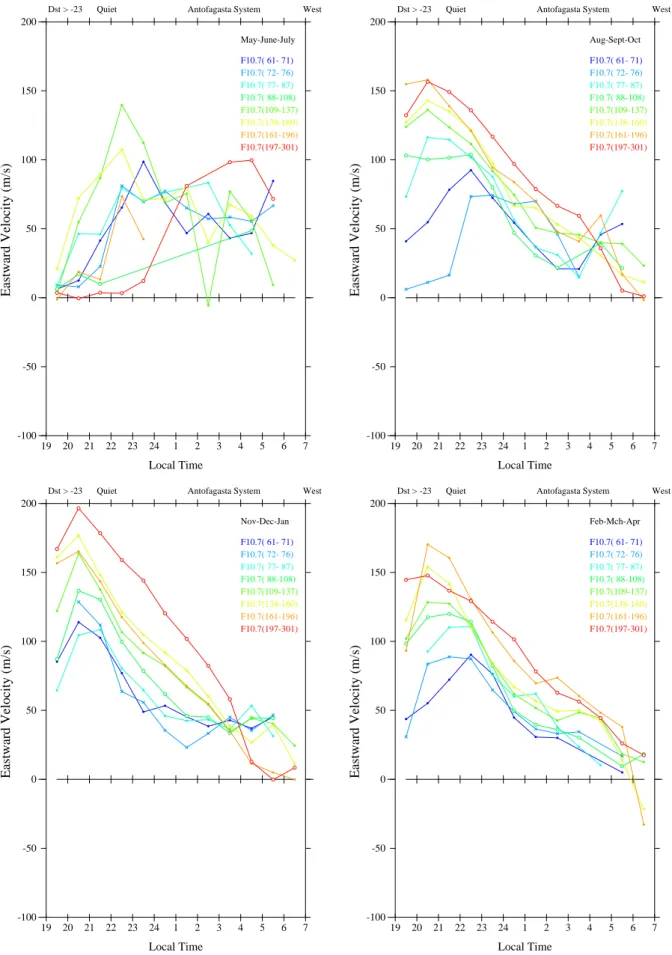
Drift velocities measured at Ancon-W from 1994 to 2001 were sorted into solar flux bins and plotted against mean lo-cal time (LT=UT−5 h). Figure 2 summarizes the results for each season. Except for the June solstice when there were fewer points, there is a broad pre-midnight peak in east-ward drift, followed by a slight post-midnight increase, or leveling off, and then a reversal to westward drift. Average drift velocities at all local times generally increase with solar flux, with the time of reversal occurring near local sunrise. The most pronounced post-midnight peak occurs during the March equinox, while during the December solstice the de-cline in eastward drift pauses before decreasing again and quickly reverses at about 05:00 local time. Similar trends are seen in Fig. 3 for Ancon-E drift data, although, as pro-posed in Sect. 5, vertical drifts contribute to the calculated drift because of the oblique ray path, and, since vertical drifts are predominantly downward after local sunset, the ob-served drifts appear consistently larger. The average drifts at Antofagasta (Fig. 4) are less consistent, and the pre-midnight peak tends to be somewhat earlier than at Ancon. The earlier peak is probably attributable to Antofagasta’s location near the eastern border of the local time zone. These results were further broken into two broad categories of Dst index to

sep-arate the effect of magnetic storms. During active conditions

(Dst<−23) at Ancon-W (Fig. 5a), the zonal drifts are

(4)

compared to quiet conditions (Fig. 5b). The post-midnight enhancement, or leveling off, is seen in all seasons and con-ditions, but is most noticeable with active conditions during the vernal equinox.

To separate the influences of geomagnetic and solar con-ditions on the statistical distribution of zonal drifts, a two-step procedure was performed on the Ancon-W data from 1994 to 2002. Drifts were sorted into 12 local time bins, and a two-dimensional, second-order fit of the drift vs. Kp

and the day of year was calculated in each bin. The drift data in each local time bin were then referenced to the model drift at a fixed Kp by subtracting the difference

be-tween the fit value of the drift and the fit value at Kp=2;

V0ref=V0−(V0fit(Kp)−V0fit(Kp=2)), where V0 is the

mea-sured drift and V0fit(Kp) is the fit value of drift. This in

effect attributes the remaining dependence to the solar flux and other unspecified variables. A second two-dimensional fit was then carried out for V0refvs. solar flux and the day of

year. A model drift for a given solar flux, Kpand day of year

can be found by reversing the steps using a set of coefficients describing the two-dimensional fits. The Appendix gives the coefficients and a more detailed description.

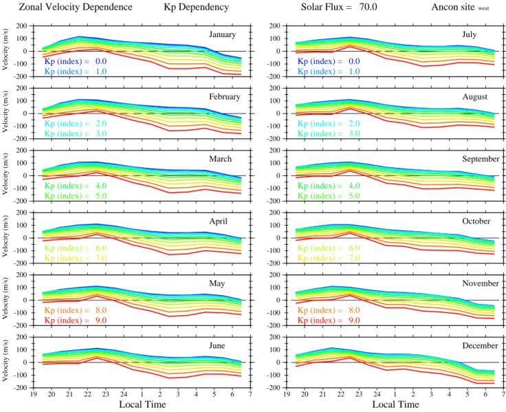
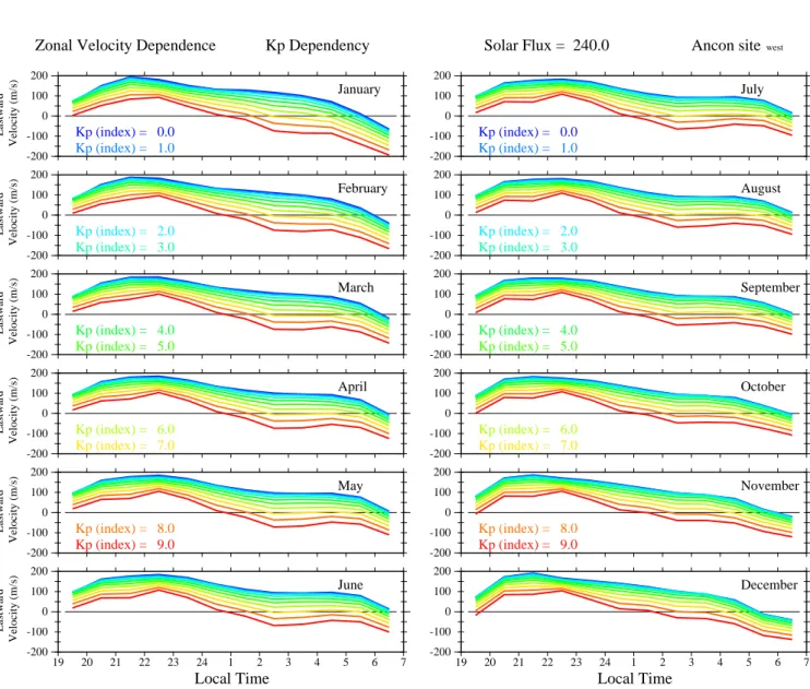
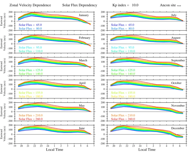
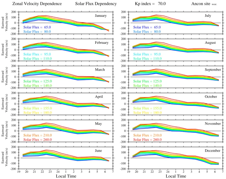
Figures 6a–d illustrate the dependence of the empirical model zonal drift on Kp and the solar flux for each month.

The Kp dependencies are shown for two extreme levels of

solar flux, and also the solar flux dependencies for quiet and active levels of Kpactivity. The drift dependencies are

simi-lar for all months, decreasing vs. Kpand increasing vs. solar

flux. These, in turn, are superimposed on the dependence on the other parameter, as seen when comparing Figs. 6a and b, and Figs. 6c and d. Further refinements to the model are pos-sible, but its main purpose is to provide a compact summary of zonal drifts at Ancon over a wide range of geophysical conditions.

4 Vertical drift

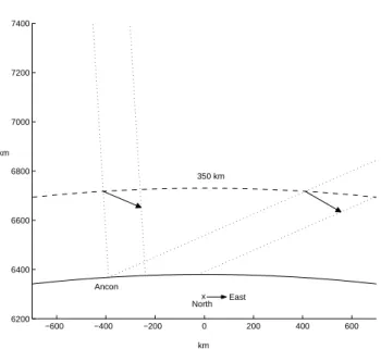
Drift velocities calculated from UHF scintillations along the low-elevation path to the east of Ancon are often larger and have more scatter than those from nearly overhead. Kil et al. (2000) noted that for ray paths at low elevation an-gles, vertical drifts contribute to the cross-correlation used for zonal drift calculations. Another effect is an overesti-mate of the zonal drift at low elevation angles caused by the Earth’s curvature. Figure 7 depicts the geometry at Ancon, where vectors at 350-km altitude represent drifting irregu-larities directly overhead and at a 28◦_{elevation angle to the}

east. The earth’s curvature in this diagram is to scale, but the drift vectors have been exaggerated for clarity; the lo-cal horizontal and vertilo-cal components of the drift velocity are assumed to be the same at each location. An additional assumption is that scattering is only weak to moderate, so that an irregularity casts a shadow-like interference pattern on the ground along the continuation of the ray path from the satellite through the irregularity (dotted lines). As seen in the figure, the “shadow” looking to the east travels farther

in a unit time than the one overhead, leading to a larger cal-culated drift velocity, V0. For purely horizontal drifts, the

angular difference in local verticals due to the Earth’s curva-ture causes an apparent downward vertical drift, as seen from Ancon looking toward the east. At an elevation angle of 28◦ and 350-km intersection altitude (ground distance ∼570 km) the difference in local verticals is ∼5◦. Therefore, for zonal drifts, velocity measurements to the east should be multiplied by a correction factor of .86.

The vertical drift at the east intersection point can be deter-mined from the measured V0and an independent

measure-ment of the horizontal drift. Figure 8 depicts the geometry at the east intersection point. The angle θ is the difference between the local horizontals at Ancon and the east intersec-tion point; ε is the elevaintersec-tion angle of the intersecintersec-tion point. The velocity perpendicular to the line of sight is the sum of the Vh and Vvcomponents in that direction; V0sin(ε)=Vh

cos(γ )+Vvsin(γ ), where γ =(90−ε−θ ) and V0 is the

mea-sured drift at Ancon. The vertical drift Vvcan then be

deter-mined from V0and Vh.

Because the Ancon-E (F8) and Antofagasta (F7) 350-km ionospheric intersection points are almost at the same mag-netic longitude (Fig. 1), Antofagasta can provide the horizon-tal drift values needed to compute vertical drifts from An-con V0measurements. Figures 9a–e are examples of vertical

drifts calculated from Antofagasta and Ancon scintillations on 7 and 9 March and 3–5 April 1997. The top panels show horizontal drift velocities at Antofagasta and Ancon looking east; the bottom panels show calculated vertical drifts and Ju-lia radar vertical drift velocities averaged over a 340–360 km altitude range in one-minute intervals, similar to the duration of scintillation samples. The Julia radar, located at Jicamarca near Ancon, detects drifting 3-m irregularities. Julia velocity points have been shifted 1.5 h, the time to travel the distance between the Julia and Antofagasta longitudes at a nominal 100 m/s zonal drift velocity. On 7 and 9 March the agree-ment between the scintillation and Julia velocities is poor, while on 3–5 April there is better agreement over extended periods. Given the uncertainty that the pattern of vertical drifts persists until it reaches the Antofagasta longitude, case by case agreement cannot be expected, especially during the dynamic growth phase of a plume. Also, because the Antofa-gasta intersection point maps to about 500 km apex altitude at the magnetic equator, height variations in horizontal drift are neglected (Pingree and Fejer, 1987; Basu et al., 1996). An alternative procedure is to use Ancon overhead V0to specify

the horizontal drift. In this case the intersection points are at the same altitude over the magnetic equator but separated in longitude by 5◦and 1 to 2 h in time.

Although individual case studies, like those in Fig. 9, show some agreement with radar measurements in the vicinity, sta-tistical results over several years would lend more credibility if they exhibited trends seen in other studies. The panel for each year in Fig. 10a shows average vertical drift velocities, computed from Antofagasta and Ancon-E data, in one-hour bins, from 00:00 to 08:00 UT, during the months of February to April, when scintillation activity is common in South

(5)

MISETA Scintillation System all Dst West 19 20 21 22 23 24 1 2 3 4 5 6 7 Local Time -100 -50 0 50 100 150 200 Eastward Velocity (m/s) F10.7( 61- 71) F10.7( 72- 76) F10.7( 77- 87) F10.7( 88-108) F10.7(109-137) F10.7(138-160) F10.7(161-196) F10.7(197-301) May-June-July

MISETA Scintillation System

all Dst West 19 20 21 22 23 24 1 2 3 4 5 6 7 Local Time -100 -50 0 50 100 150 200 Eastward Velocity (m/s) F10.7( 61- 71) F10.7( 72- 76) F10.7( 77- 87) F10.7( 88-108) F10.7(109-137) F10.7(138-160) F10.7(161-196) F10.7(197-301) Aug-Sept-Oct

all Dst West 19 20 21 22 23 24 1 2 3 4 5 6 7 Local Time Eastward Velocity (m/s) -100 -50 0 50 100 150 200 F10.7( 61- 71) F10.7( 72- 76) F10.7( 77- 87) F10.7( 88-108) F10.7(109-137) F10.7(138-160) F10.7(161-196) F10.7(197-301) Nov-Dec-Jan

all Dst West 19 20 21 22 23 24 1 2 3 4 5 6 7 Local Time Eastward Velocity (m/s) -100 -50 0 50 100 150 200 F10.7( 61- 71) F10.7( 72- 76) F10.7( 77- 87) F10.7( 88-108) F10.7(109-137) F10.7(138-160) F10.7(161-196) F10.7(197-301) Feb-Mch-Apr

(6)

MISETA Scintillation System all Dst East 19 20 21 22 23 24 1 2 3 4 5 6 7 Local Time -100 -50 0 50 100 150 200 Eastward Velocity (m/s) F10.7( 61- 71) F10.7( 72- 76) F10.7( 77- 87) F10.7( 88-108) F10.7(109-137) F10.7(138-160) F10.7(161-196) F10.7(197-301) May-June-July

all Dst East 19 20 21 22 23 24 1 2 3 4 5 6 7 Local Time -100 -50 0 50 100 150 200 Eastward Velocity (m/s) F10.7( 61- 71) F10.7( 72- 76) F10.7( 77- 87) F10.7( 88-108) F10.7(109-137) F10.7(138-160) F10.7(161-196) F10.7(197-301) Aug-Sept-Oct

all Dst East 19 20 21 22 23 24 1 2 3 4 5 6 7 Local Time -100 -50 0 50 100 150 200 Eastward Velocity (m/s) F10.7( 61- 71) F10.7( 72- 76) F10.7( 77- 87) F10.7( 88-108) F10.7(109-137) F10.7(138-160) F10.7(161-196) F10.7(197-301) Nov-Dec-Jan

all Dst East 19 20 21 22 23 24 1 2 3 4 5 6 7 Local Time -100 -50 0 50 100 150 200 Eastward Velocity (m/s) F10.7( 61- 71) F10.7( 72- 76) F10.7( 77- 87) F10.7( 88-108) F10.7(109-137) F10.7(138-160) F10.7(161-196) F10.7(197-301) Feb-Mch-Apr

(7)

Antofagasta System Dst > -23 Quiet West 19 20 21 22 23 24 1 2 3 4 5 6 7 Local Time -100 -50 0 50 100 150 200 Eastward Velocity (m/s) F10.7( 61- 71) F10.7( 72- 76) F10.7( 77- 87) F10.7( 88-108) F10.7(109-137) F10.7(138-160) F10.7(161-196) F10.7(197-301) May-June-July Antofagasta System Dst > -23 Quiet West 19 20 21 22 23 24 1 2 3 4 5 6 7 Local Time -100 -50 0 50 100 150 200 Eastward Velocity (m/s) F10.7( 61- 71) F10.7( 72- 76) F10.7( 77- 87) F10.7( 88-108) F10.7(109-137) F10.7(138-160) F10.7(161-196) F10.7(197-301) Aug-Sept-Oct Antofagasta System Dst > -23 Quiet West 19 20 21 22 23 24 1 2 3 4 5 6 7 Local Time -100 -50 0 50 100 150 200 Eastward Velocity (m/s) F10.7( 61- 71) F10.7( 72- 76) F10.7( 77- 87) F10.7( 88-108) F10.7(109-137) F10.7(138-160) F10.7(161-196) F10.7(197-301) Nov-Dec-Jan Antofagasta System Dst > -23 Quiet West 19 20 21 22 23 24 1 2 3 4 5 6 7 Local Time -100 -50 0 50 100 150 200 Eastward Velocity (m/s) F10.7( 61- 71) F10.7( 72- 76) F10.7( 77- 87) F10.7( 88-108) F10.7(109-137) F10.7(138-160) F10.7(161-196) F10.7(197-301) Feb-Mch-Apr

(8)

MISETA Scintillation System Dst < -23 Active West 19 20 21 22 23 24 1 2 3 4 5 6 7 Local Time -100 -50 0 50 100 150 200 Eastward Velocity (m/s) F10.7( 61- 71) F10.7( 72- 76) F10.7( 77- 87) F10.7( 88-108) F10.7(109-137) F10.7(138-160) F10.7(161-196) F10.7(197-301) May-June-July

Dst < -23 Active West 19 20 21 22 23 24 1 2 3 4 5 6 7 Local Time -100 -50 0 50 100 150 200 Eastward Velocity (m/s) F10.7( 61- 71) F10.7( 72- 76) F10.7( 77- 87) F10.7( 88-108) F10.7(109-137) F10.7(138-160) F10.7(161-196) F10.7(197-301) Aug-Sept-Oct

Dst < -23 Active West 19 20 21 22 23 24 1 2 3 4 5 6 7 Local Time -100 -50 0 50 100 150 200 Eastward Velocity (m/s) F10.7( 61- 71) F10.7( 72- 76) F10.7( 77- 87) F10.7( 88-108) F10.7(109-137) F10.7(138-160) F10.7(161-196) F10.7(197-301) Nov-Dec-Jan

Dst < -23 Active West 19 20 21 22 23 24 1 2 3 4 5 6 7 Local Time -100 -50 0 50 100 150 200 Eastward Velocity (m/s) F10.7( 61- 71) F10.7( 72- 76) F10.7( 77- 87) F10.7( 88-108) F10.7(109-137) F10.7(138-160) F10.7(161-196) F10.7(197-301) Feb-Mch-Apr

(9)

MISETA Scintillation System Dst > -23 Quiet West 19 20 21 22 23 24 1 2 3 4 5 6 7 Local Time -100 -50 0 50 100 150 200 Eastward Velocity (m/s) F10.7( 61- 71) F10.7( 72- 76) F10.7( 77- 87) F10.7( 88-108) F10.7(109-137) F10.7(138-160) F10.7(161-196) F10.7(197-301) May-June-July

Dst > -23 Quiet West 19 20 21 22 23 24 1 2 3 4 5 6 7 Local Time -100 -50 0 50 100 150 200 Eastward Velocity (m/s) F10.7( 61- 71) F10.7( 72- 76) F10.7( 77- 87) F10.7( 88-108) F10.7(109-137) F10.7(138-160) F10.7(161-196) F10.7(197-301) Aug-Sept-Oct

Dst > -23 Quiet West 19 20 21 22 23 24 1 2 3 4 5 6 7 Local Time -100 -50 0 50 100 150 200 Eastward Velocity (m/s) F10.7( 61- 71) F10.7( 72- 76) F10.7( 77- 87) F10.7( 88-108) F10.7(109-137) F10.7(138-160) F10.7(161-196) F10.7(197-301) Nov-Dec-Jan

Dst > -23 Quiet West 19 20 21 22 23 24 1 2 3 4 5 6 7 Local Time -100 -50 0 50 100 150 200 Eastward Velocity (m/s) F10.7( 61- 71) F10.7( 72- 76) F10.7( 77- 87) F10.7( 88-108) F10.7(109-137) F10.7(138-160) F10.7(161-196) F10.7(197-301) Feb-Mch-Apr

(10)

Zonal Velocity Dependence Kp Dependency Solar Flux = 70.0 Ancon sitewest January 200 100 0 -100 -200 Eastward

Velocity (m/s) Kp (index) = 0.0_{Kp (index) = 1.0}

February 200 100 0 -100 -200 Eastward

March 200 100 0 -100 -200 Eastward

April 200 100 0 -100 -200 Eastward

May 200 100 0 -100 -200 Eastward

June Local Time 19 20 21 22 23 24 1 2 3 4 5 6 7 200 100 0 -100 -200 Eastward Velocity (m/s) July 200 100 0 -100 -200 Kp (index) = 0.0 Kp (index) = 1.0 August 200 100 0 -100 -200 Kp (index) = 2.0 Kp (index) = 3.0 September 200 100 0 -100 -200 Kp (index) = 4.0 Kp (index) = 5.0 October 200 100 0 -100 -200 Kp (index) = 6.0 Kp (index) = 7.0 November 200 100 0 -100 -200 Kp (index) = 8.0 Kp (index) = 9.0 December Local Time 19 20 21 22 23 24 1 2 3 4 5 6 7 200 100 0 -100 -200

(11)

Zonal Velocity Dependence Kp Dependency Solar Flux = 240.0 Ancon sitewest January 200 100 0 -100 -200 Eastward

March 200 100 0 -100 -200 Eastward

April 200 100 0 -100 -200 Eastward

May 200 100 0 -100 -200 Eastward

June Local Time 19 20 21 22 23 24 1 2 3 4 5 6 7 200 100 0 -100 -200 Eastward Velocity (m/s) July 200 100 0 -100 -200 Kp (index) = 0.0 Kp (index) = 1.0 August 200 100 0 -100 -200 Kp (index) = 2.0 Kp (index) = 3.0 September 200 100 0 -100 -200 Kp (index) = 4.0 Kp (index) = 5.0 October 200 100 0 -100 -200 Kp (index) = 6.0 Kp (index) = 7.0 November 200 100 0 -100 -200 Kp (index) = 8.0 Kp (index) = 9.0 December Local Time 19 20 21 22 23 24 1 2 3 4 5 6 7 200 100 0 -100 -200

(12)

Zonal Velocity Dependence Solar Flux Dependency Kp index = 10.0 Ancon sitewest January 200 100 0 -100 -200 Eastward

Velocity (m/s) Solar Flux = 65.0_{Solar Flux = 80.0}

March 200 100 0 -100 -200 Eastward

April 200 100 0 -100 -200 Eastward

May 200 100 0 -100 -200 Eastward

June Local Time 19 20 21 22 23 24 1 2 3 4 5 6 7 200 100 0 -100 -200 Eastward Velocity (m/s) July 200 100 0 -100 -200 Solar Flux = 65.0 Solar Flux = 80.0 August 200 100 0 -100 -200 Solar Flux = 95.0 Solar Flux = 110.0 September 200 100 0 -100 -200 Solar Flux = 125.0 Solar Flux = 140.0 October 200 100 0 -100 -200 Solar Flux = 155.0 Solar Flux = 180.0 November 200 100 0 -100 -200 Solar Flux = 210.0 Solar Flux = 260.0 December Local Time 19 20 21 22 23 24 1 2 3 4 5 6 7 200 100 0 -100 -200

(13)

Zonal Velocity Dependence Solar Flux Dependency Kp index = 70.0 Ancon sitewest January 200 100 0 -100 -200 Eastward

March 200 100 0 -100 -200 Eastward

April 200 100 0 -100 -200 Eastward

May 200 100 0 -100 -200 Eastward

June Local Time 19 20 21 22 23 24 1 2 3 4 5 6 7 200 100 0 -100 -200 Eastward Velocity (m/s) July 200 100 0 -100 -200 Solar Flux = 65.0 Solar Flux = 80.0 August 200 100 0 -100 -200 Solar Flux = 95.0 Solar Flux = 110.0 September 200 100 0 -100 -200 Solar Flux = 125.0 Solar Flux = 140.0 October 200 100 0 -100 -200 Solar Flux = 155.0 Solar Flux = 180.0 November 200 100 0 -100 -200 Solar Flux = 210.0 Solar Flux = 260.0 December Local Time 19 20 21 22 23 24 1 2 3 4 5 6 7 200 100 0 -100 -200

(14)

−600 −400 −200 0 200 400 600 6200 6400 6600 6800 7000 7200 7400 East 350 km Ancon km km x North

Fig. 7. View geometry from Ancon (approximately to scale). Dot-ted lines indicate ray paths intersecDot-ted by drifting irregularities viewed nearly overhead and low to the east.

ε Vo Vv Vh θ γ

Fig. 8. Geometry at the Ancon-E ionospheric intersection point. Irregularities with horizontal and vertical drift components Vhand

Vv, respectively, yield a calculated V0at Ancon-E.

0 1 2 3 4 5 6 7 8 9 10 −50 0 50 100 150 200 1997/03/07 Vo(m/s) UT Ancon east Antofagasta 0 1 2 3 4 5 6 7 8 9 10 −100 −50 0 50 100 Vv(m/s) UT Julia Calculated

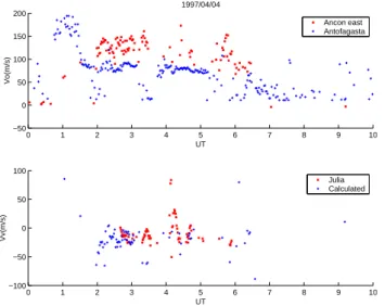
Fig. 9. (a) Top panel: Observed V0 drift velocities at Ancon-E and Antofagasta on 7 March 1997. Bottom panel: Observed Julia radar vertical drifts and vertical drifts calculated from Ancon-E and Antofagasta V0in top panel. Julia data is displaced 1.5 h later to account for zonal drift.

(15)

Fig. 9. (c) Same as Fig. 9a for 3 April 1997.

Fig. 9. (d) Same as Fig. 9a for 4 April 1997.

Fig. 9. (e) Same as Fig. 9a for 5 April 1997.

0 2 4 6 8

−100 −50 0 50

02/01 − 05/31 (Antofagasta, Ancon east)

Vz(m/s) UT 1997 102 386 443 323 315 199 69 0 2 4 6 8 −100 −50 0 50 Vz(m/s) UT 1998 234 948 1233 1050 881 513 215 119 0 2 4 6 8 −100 −50 0 50 Vz(m/s) UT 1999 485 1466 1701 1767₁₁₈₁716 414 112 0 2 4 6 8 −100 −50 0 50 Vz(m/s) UT 2000 258 704 917 914 826 582 464 342 0 2 4 6 8 −100 −50 0 50 Vz(m/s) UT 2001 238 1010 1258 1200 972 555 278 177

Fig. 10. (a) Average vertical drift calculated from Antofagasta and

Ancon-E V0data vs. UT for the months February–May from 1997

(16)

0 2 4 6 8 −100

−50 0 50

03/01 − 05/29 (Ancon west, Ancon east)

Vz(m/s) UT 1997 107 412 547 433 354 157 58 0 2 4 6 8 −100 −50 0 50 Vz(m/s) UT 1998 50 470 712 543 356 144 18 3 0 2 4 6 8 −100 −50 0 50 Vz(m/s) UT 1999 195 1001 1088 1065 665 178 37 33 0 2 4 6 8 −100 −50 0 50 Vz(m/s) UT 2000 54 576 ₇₇₂ 831 673 480 299 204 0 2 4 6 8 −100 −50 0 50 Vz(m/s) UT 2001 64 ₆₆₉ 921 799 590 194 97 69

Fig. 10. (b) Same as Fig. 10a except data is from Ancon-W instead of Antofagasta.

America, and also including cases occurring in May. These results can be compared with equinox statistics from Fig. 1 in Fejer et al. (1991), which shows Jicamarca velocities that are generally negative (downward) from 20:00 to 03:00 LT (01:00 to 08:00 UT in Fig. 10a). In Fig. 10b Ancon-W sup-plies the horizontal velocity; the results are similar except that vertical drifts are somewhat less negative in 2000–2001. Since Ancon-E data is common to both figures, differences result from the horizontal drift data source, each of which suffers from its own drawback mentioned above. The Jica-marca data range from about −20 to −60 m/s for solar fluxes ranging from less than 100 to greater than 150, indicating that the more negative drifts in Figs. 10a and b around the year 2000 are consistent with increased solar activity. Val-ladares et al. (1996) found systematic differences between zonal drifts measured by incoherent radar and scintillation techniques which may apply to the vertical drifts as well. The vertical drift statistics include all geomagnetic and so-lar conditions and have rather so-large error bars that make the UT trend in each year suggestive but not definite.

5 Conclusions and discussion

The zonal drift statistics presented here update the first re-sults of Valladares et al. (1996) through the current so-lar maximum. As noted by Fejer et al. (1985), eastward zonal drift velocities measured by the Jicamarca incoherent radar are generally slower than those seen by two spaced re-ceivers. Figure 11 shows a linear fit of all the Ancon spaced-receiver zonal drift data (1994–2002) vs. solar flux during the equinoxes at 02:00 LT, generally the time of maximum eastward velocity. Each solar flux bin of 10 units has 1000 or more points up to flux=205 and over 200 points up to flux=245. A similar plot of the Jicamarca eastward peak ve-locity (Fig. 8 in Fejer et al., 1991) has comparable error bars,

50 100 150 200 250 300 0 50 100 150 200 250 m = 0.49 b = 72.33

Ancon Zonal Drift (equinoxes)

V0(m/s)

f107

Fig. 11. Linear fit to Ancon zonal drift measurements in 02:00 LT bin vs. solar flux during the equinoxes (all data 1994–2002).

a slope of 0.45 and an intercept at 60.01 m/s. The higher in-tercept and slightly steeper slope in Fig. 11 confirm that aver-age spaced-receiver drifts are about 10–20 m/s faster than the average Jicamarca drifts. In Fig. 11 the average drift stops in-creasing and remains at approximately 150 m/s when the so-lar flux exceeds 200, which indicates that the second-order fit in the empirical model presented here is a better approxima-tion than a linear fit. However, the relatively large error bars for the solar flux and the Kpdependences mean that a broad

range of drift velocities are associated with these global in-dices and the details depend more on local dynamic condi-tions.

After the installation of the Ancon-E antennas, it was noted that the measured drift velocities to the east were usu-ally greater and more variable than the zonal drifts seen by Ancon-W nearly overhead. It was realized that, in addition to the longer path through the ionosphere, the viewing geome-try could introduce contributions from real vertical drifts and an apparent vertical drift due to the Earth’s curvature. This conclusion assumes mostly forward scatter of radio waves by km-scale irregularities that produce interference patterns on the ground and cause UHF scintillations. Furthermore, the km-scale ionospheric irregularities are assumed to drift both horizontally and vertically with the ambient plasma (frozen-in condition), the same drift that is seen by (frozen-incoherent scatter radars. The characteristics of the zonal drift model presented here are well established and generally agree with the statis-tics of published radar data.

The results for vertical drifts from UHF measurements are encouraging, but tentative, and several questions remain. First, there is the applicability of the simple geometry used here, which should be compared with a full treatment of slant propagation through a real ionosphere. For low elevation an-gles, however, the approximations in propagation models like Costa and Basu (2002) and similar studies probably would not be valid. Second, Bhattacharyya et al. (2001) noted that

(17)

Table 1. Model coefficients for equation A2 Kp* LT C1 C2 C3 C4 C5 C6 XBAR YBAR SS 19:00–20:00 85.18 1.00 −5.15 −1.26 −1.32 −25.00 213.78 23.94 40.29 20:00–21:00 125.08 2.40 −19.74 0.12 0.55 −18.71 203.05 21.86 41.93 21:00–22:00 130.41 1.84 −23.81 1.68 0.28 −21.44 194.61 20.99 42.78 22:00–23:00 126.47 0.13 −23.57 0.20 1.71 −10.54 193.75 21.23 44.14 23:00–00:00 109.54 0.15 −24.09 −0.22 0.61 −19.15 193.25 21.03 43.63 00:00–01:00 82.34 1.10 −22.87 1.19 −0.15 −31.31 190.26 21.18 43.97 01:00–02:00 59.63 1.54 −27.13 2.25 1.81 −27.18 187.58 20.02 42.99 02:00–03:00 52.03 1.37 −29.78 2.27 4.06 −39.97 189.75 21.17 44.41 03:00–04:00 48.94 0.97 −28.19 1.52 4.58 −43.12 199.09 24.33 44.90 04:00–05:00 48.60 −2.31 −32.67 −0.92 2.02 −23.31 205.09 25.86 39.44 05:00–06:00 34.15 −6.49 −29.17 −3.44 2.12 −21.03 204.14 28.37 37.25 06:00–07:00 0.66 −4.34 −28.12 −3.33 1.56 −19.43 210.80 30.45 38.01 Solar Flux LT C1 C2 C3 C4 C5 C6 XBAR YBAR SS 19:00–20:00 92.72 0.77 23.28 −4.27 −2.99 −11.74 213.78 119.51 67.91 20:00–21:00 136.96 3.24 47.66 −0.24 1.64 −22.29 203.05 132.99 76.27 21:00–22:00 142.76 1.21 43.37 3.76 −0.07 −16.90 194.61 138.25 79.85 22:00–23:00 137.32 −1.79 36.54 −2.40 −1.04 −5.10 193.75 137.78 80.99 23:00–24:00 118.36 −1.81 35.47 −4.06 1.15 −0.24 193.25 136.35 81.44 00:00–01:00 92.67 −0.01 33.25 0.06 1.71 −0.74 190.26 138.99 81.98 01:00–02:00 70.76 1.77 30.09 3.93 −0.94 −1.09 187.58 144.99 82.90 02:00–03:00 64.78 1.96 26.66 3.82 −2.39 −4.50 189.75 150.70 83.70 03:00–04:00 64.40 −1.03 26.49 0.14 0.15 −4.05 199.09 147.60 81.91 04:00–05:00 60.15 −7.42 23.00 −6.58 1.42 −1.59 205.09 141.71 75.73 05:00–06:00 44.12 −14.05 17.84 −13.92 0.71 −0.43 204.14 133.40 68.85 06:00–07:00 10.83 −8.78 7.16 −10.90 2.94 −4.76 210.80 135.80 66.02

spaced antenna drift velocities might not reflect the ambient plasma drift during the turbulent early stage of plasma bub-ble development, which typically occurs before 22:00 LT. In fact, the top panels of Figs. 9a–e show that the drift measured by Ancon-E fluctuates considerably more than the zonal drift at Antofagasta at all local times, which indicates that the ver-tical motion of the irregularities is generally more variable than the zonal drift. The variability, as seen in the lower pan-els of Figs. 8a–e, is similar to the Julia data at most times. Finally, the horizontal velocities used in the calculations are not at the Ancon-E ionospheric intersection point, but either at a higher altitude, when coming from the Antofagasta data, or at a different longitude, when coming from the Ancon-W data.

Appendix A

The model drift at Ancon for a desired solar flux and Kp* is

given by

Vmodel=Vfit(solar f lux)

+(Vfit(Kp∗)−Vfit(Kp∗=20)),

(A1)

where Kp*=10 Kp and Kp=0., 0.33, 0.67, 1.00, . . . . Each

velocity term, Vfit, is expressed in terms of the row of

coeffi-cients for a local time in the appropriate table.

Vfit=C1+C2X + C3Y + C4X2+C5XY + C6Y2 (A2)

X=(DOY–XBAR)/SS, where DOY = day of year (1–365). Y=(GPH–YBAR)/SS, where GPH = geophysical parameter (solar flux or Kp*).

Acknowledgements. We thank J. Espinoza and R. Villafani for their dedication to the smooth operation of the spaced receiver

scintil-lation instrument at Ancon, Peru. This material is based upon

work supported by the NSF under Grants 0123560 and 0243294. The work at Boston College was also partially supported by Air Force Research Laboratory contract F19628-02-C-0087, AFOSR task 2311AS. The observatory at Ancon is operated by the Geo-physical Institute of Peru, Ministry of Education. The Jicamarca Radio Observatory is operated by the Geophysical Institute of Peru, Ministry of Education, with support from the National Science Foundation Cooperative Agreement ATM-9911209 through Cornell University.

Topical Editor M. Lester thanks W. R. Coley and another referee for their help in evaluating this paper.

(18)

References

Basu, S., Kudeki, E., Basu, S., Valladares, C. E., Weber, E. J., Zengingonul, H. P., Bhattacharyya, S., Sheehan, R., Meriwether, J. W., Biondi, M. A., Kuenzler, H., and Espinoza, J.: Scintil-lations, plasma drifts, and neutral winds in the equatorial iono-sphere after sunset, J. Geophys. Res., 101, 26 795–26 809, 1996. Bhattacharyya, A., Basu, S., Groves, K. M., Valladares, C. E., and Sheehan, R.: Dynamics of equatorial F-region irregularities from spaced receiver scintillation observations, Geophys. Res. Lett., 28, 119–122, 2001.

Coley, W. R. and Heelis, R. A.: Low-latitude zonal and vertical ion drifts seen by DE 2, J. Geophys. Res., 6751, 1989.

Costa, E. and Basu, S.: A radio wave scattering algorithm and irregularity model for scintillation predictions, Radio Sci., 37, 10.1029, 2002.

Eccles, J. V.: A simple model of low latitude electric fields, J. Geo-phys. Res., 103, 26 699–26 708, 1998.

Fejer, B. G., de Paula, E. R., Gonzalez, S. A., and Woodman, R. R.: Average vertical and zonal F-region plasma drifts over Jica-marca, J. Geophys. Res., 96, 13 901, 1991.

Fejer, B. G., Farley, D. T., Gonzales, C. A., Woodman, R. F., and Calderon, C.: F-region east-west drifts at Jicamarca, J. Geophys. Res., 86, 215, 1981.

Fejer, B. G., Kudeki, E., and Farley, D. T.: Equatorial F-region zonal plasma drifts, J. Geophys. Res., 90, 12 249–12 255, 1985. Fejer, B. G. and Scherliess, L.: Empirical models of storm time

equatorial zonal electric fields, J. Geophys. Res., 102, 24 047– 24 056, 1997.

Fejer, B. G. and Scherliess, L.: Mid- and low latitude prompt-penetration ionospheric zonal plasma drifts, Geophys. Res. Lett., 25, 3071, 1998.

Fejer, B. G., Scherliess, L., and de Paula, E. R.: Effects of the verti-cal plasma drift velocity on the generation and evolution of equa-torial spread F, J. Geophys. Res., 104, 19 859–19 869, 1999. Kil, H., Kintner, P. M., de Paula, E. R., and Kantor, I. J.: Global

positioning system measurements of the ionospheric zonal ap-parent velocity at Cachoeira Paulista in Brazil, J. Geophys. Res., 105, 5317–5327, 2000.

Pingree, J. E. and Fejer, B. G.: On the height variation of the equa-torial F-region vertical plasma drifts, J. Geophys. Res., 92, 4763, 1987.

Rishbeth, H.: Polarization fields produced by winds in the equato-rial F-region, Planet Space Sci., 19, 357–369, 1971.

Rishbeth, H.: The F-region dynamo, J. Atmos. Terr. Phys., 43, 387– 392, 1981.

Scherliess, L. and Fejer, B. G.: Radar and satellite global equatorial F-region vertical drift model, J. Geophys. Res., 104, 6829–6842, 1999.

Vacchione, J. D., Franke, S. J., and Yeh, K. C.: A new analysis technique for estimating zonal irregularity drifts and variability in the equatorial F-region using spaced receiver scintillation data, Radio Sci., 22, 745, 1987.

Valladares, C. E., Meriwether, J. W., Sheehan, R., and Biondi, M. A.: Correlative study of neutral winds and scintillation drifts measured near the magnetic equator, J. Geophys. Res., 107, A7, 10.1029, 2002.

Valladares, C. E., Sheehan, R., Basu, S., Kuenzler, H., and Es-pinoza, J.: The multi-instrumented studies of equatorial ther-mosphere aeronomy scintillation system: Climatology of zonal drifts, J. Geophys. Res., 101, 26 939, 1996.