The hydro-meteorological chain in Piemonte region, North Western Italy - analysis of the HYDROPTIMET test cases

(1)

HAL Id: hal-00299307

https://hal.archives-ouvertes.fr/hal-00299307

Submitted on 3 Nov 2005

HAL is a multi-disciplinary open access

archive for the deposit and dissemination of

sci-entific research documents, whether they are

pub-lished or not. The documents may come from

teaching and research institutions in France or

abroad, or from public or private research centers.

L’archive ouverte pluridisciplinaire HAL, est

destinée au dépôt et à la diffusion de documents

scientifiques de niveau recherche, publiés ou non,

émanant des établissements d’enseignement et de

recherche français ou étrangers, des laboratoires

publics ou privés.

The hydro-meteorological chain in Piemonte region,

North Western Italy - analysis of the HYDROPTIMET

test cases

D. Rabuffetti, M. Milelli

To cite this version:

D. Rabuffetti, M. Milelli. The hydrometeorological chain in Piemonte region, North Western Italy

-analysis of the HYDROPTIMET test cases. Natural Hazards and Earth System Science, Copernicus

Publications on behalf of the European Geosciences Union, 2005, 5 (6), pp.845-852. �hal-00299307�

(2)

SRef-ID: 1684-9981/nhess/2005-5-845 European Geosciences Union

and Earth

System Sciences

The hydro-meteorological chain in Piemonte region, North Western

Italy – analysis of the HYDROPTIMET test cases

D. Rabuffetti and M. Milelli

ARPA Piemonte, Corso Unione Sovietica, 216, 10134 Torino, Italy

Received: 19 July 2005 – Revised: 13 October 2005 – Accepted: 13 October 2005 – Published: 3 November 2005 Part of Special Issue “HYDROPTIMET”

Abstract. The HYDROPTIMET Project, Interreg IIIB EU program, is developed in the framework of the prediction and prevention of natural hazards related to severe hydro-meteorological events and aims to the optimisation of Hydro-Meteorological warning systems by the experimentation of new tools (such as numerical models) to be used opera-tionally for risk assessment. The objects of the research are the mesoscale weather phenomena and the response of watersheds with size ranging from 102 to 103 km2. Non-hydrostatic meteorological models are used to catch such phenomena at a regional level focusing on the Quantita-tive Precipitation Forecast (QPF). Furthermore hydrological Quantitative Discharge Forecast (QDF) are performed by the simulation of run-off generation and flood propagation in the main rivers of the territory. In this way observed data and QPF are used, in a real-time configuration, for one-way forcing of the hydrological model that works operationally connected to the Piemonte Region Alert System. The main hydro-meteorological events that affected Piemonte Region in the last years are analysed, these are the HYDROPTI-MET selected test cases of 14–18 November 2002 and 23– 26 November 2002. The results obtained in terms of QPF and QDF offer a basis to evaluate the sensitivity of the whole hydro-meteorological chain to the uncertainties in the numer-ical simulations. Different configurations of non-hydrostatic meteorological models are also evaluated.

1 Introduction

HYDROPTIMET (OPTimisation of HYDRO-METeoro-logical models) is an European MEDOCC INTERREG III Project and ARPA Piemonte is the coordinator. The territory involved in the activities of the project is well distributed along the Mediterranean coast and includes the regions of the western part of the Alps subject to severe events and to strong vulnerability due to the complex orography. The main

Correspondence to: D. Rabuffetti

(d.rabuffetti@arpa.piemonte.it)

subject of the research is the forecast of floods in little and medium sized quick responding catchments.

For such catchments the space-time scale dichotomy be-tween meteorological outputs and hydrological requirements is very high (Ferraris et al., 2002) resulting in often uncer-tain discharge forecasts and, as a consequence, in not reliable risk assessment. Uncertainty sources are found either in the meteorological input as well as in the hydrological concep-tualisation and parameters. From a theoretical point of view a probabilistic approach should be considered (Krzysztofow-icz, 1999) event though it often produce big difficulties in warning dissemination (Parker and Fordham, 1996). In this work a deterministic hydrometeorological chain is adopted because the aim is to understand the role and the weight of the different uncertainty sources in an operational frame, rather than to propose a new or a better approach. In fact the hydrological simulation and the alert system are here used for validation purposes (Jasper and Kaufmann, 2003) allow-ing an objective comparison between results obtained usallow-ing different configuration of the chain. In particular different Lokal Modell set up are used and compared with the ‘perfect meteorological forecast’ results.

The events here described (the HYDROPTIMET selected test cases of 14–18 November 2002 and 23–26 November 2002) mainly affected little and medium-sized catchments and the superposition of their flood waves produced signif-icant effects on the main rivers only in the nearby of the confluences. On the whole these events did not produce ex-treme floods but can be considered as lower thresholds above which floods will became very dangerous. It is for this rea-son that it seems very important to understand the capabil-ity of the system to forecast such events. The case study occurred in Piemonte (north-west of Italy), a predominantly alpine region covering 25 000 km2. Piemonte is situated on the Padana plain and bounded on three sides by mountain chains covering 73% of its territory (Fig. 1). On the basis of historical data, available since the year 1800, Piemonte is hit by calamitous meteorological events, on average, once every two years.

(3)

846 D. Rabuffetti and M. Milelli: The hydro-meteorological chain in Piemonte

Table 1. Sketch of meteorological runs characteristics (see also Fig. 1).

Domain

Initial and boundary condition Large Small

ECMWF (European Centre for Medium-range Weather Forecasts, Reading, UK) S4 S2

GME (Global Modell Ersatz, Offenbach, Germany) S3 S1

Figure 1. Piemonte location (in the black circle, indicated by the white arrow) with the domains of integration of the four meteorological simulations (s1 and s2 in red, s3 and s4 in black).

17 Fig. 1. Piemonte location (in the black circle, indicated by the white

arrow) with the domains of integration of the four meteorological simulations (s1 and s2 in red, s3 and s4 in black).

2 Meteorological analysis

The goal of the meteorological activities at ARPA Piemonte is the study of different configurations of the meteorological model Lokal Modell (LM), in order to optimise the QPF over the Piemonte warning areas. This variable is quite important since it is the input for the hydrological models used to assess flood risk level.

Lokal Modell is a non-hydrostatic limited area model which is developed and maintained into the COSMO (COn-sortium for Small-scale MOdelling) project by Germany, Italy, Switzerland, Poland and Greece. In Italy, the model has been implemented by UGM (the national meteorolog-ical service), ARPA Piemonte and ARPA SIM (regional weather services). Such a model is based on the primitive hydro-thermodynamical equations describing compressible non-hydrostatic flow in a moist atmosphere without any scale approximations. In fact the use of non-hydrostatic compress-ible (i.e. unfiltered) dynamical equations allows to avoid re-strictions on the spatial scales and on the domain size. The equation of the vertical moment is not approximate, so that it can describe much better those phenomena for which it is important to take into account the vertical velocity: thunder-storms, katabatic winds, and all the phenomena that occur in the lower atmosphere. Moreover, the use of a fine grid (7 km instead of 40 as it is in the global models) permits a better definition of the orography, which is a real problem in areas

where there are sharp slopes from the coast to the mountains. The basic equations are written in advection form and the continuity equation is replaced by a prognostic equation for the perturbation pressure (i.e. the deviation of pressure from the reference state). The model equations are solved numer-ically using the traditional finite difference method.

The model derives directly (prognostically) the velocity, the temperature, the pressure perturbation, the specific hu-midity and the water content in the clouds; instead, it calcu-lates (diagnostically) the total air density and the precipita-tion fluxes of rain and snow. There is a generalized terrain-following height-coordinate in the vertical direction, use-ful to describe the complex orography regions. The initial and boundary conditions are interpolated opportunely from a global model with coarser horizontal and vertical resolu-tion and larger domain of integraresolu-tion. A variety of subgrid-scale physical processes are taken into account by parame-terisation schemes which are not described here (Doms et al., 2005). For a more exhaustive description of the model and of the organization of the Consortium, see for instance the COSMO Newsletter No. 5 available at the official web site http://www.cosmo-model.org.

The Italian operational configuration of LM (named LAMI) at 7 km (0.0625◦)grid spacing is the following:

– rotated lat-lon coordinates with 234×272 grid points; – 35 vertical layers;

– boundary conditions given by GME (Global Modell Er-satz, Offenbach, Germany) updated every hour (one-way forcing);

– initial conditions given by a nudging-based assimilation suite (Schraff et al., 2004) which includes two 12-h cy-cles with AOF-file provided by UGM Rome with SYN-OPs, AIREPs, TEMPs and PILOTs;

– two forecasts up to 72 h, at 00:00 and 12:00 UTC, per-formed daily starting from the analyses provided by the assimilation cycles.

We used here LM v3.5 which is a more recent version with respect to the one running at the time of the events. This model has been already extensively verified over Piemonte and Northern Italy since it is the operational tool for the fore-cast production at ARPA Piemonte (see for instance Milelli et al., 2003).

The configuration of the s1 runs performed here (see Ta-ble 1) is the same as for the operational one but without

(4)

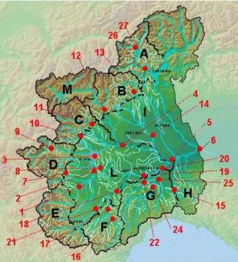
Fig. 2. Homogeneous alert areas, river network and location of the

27 cross sections considered.

assimilation cycle and truncated to +36 h; concerning s2, the only difference with respect to s1, is the “father” global model which in this case is the ECMWF model (European Centre for Medium-range Weather Forecasts, Reading, UK), with boundary conditions updated every three hours. The runs s3 and s4 are similar to s1 and s2, respectively, but with a larger domain (325×325 grid points). The latter has been se-lected in order to have the Piemonte region in the centre and avoiding possible interference problems with the borders.

The simulations have been carried out on two events of in-tense precipitation that occurred in the North-West of Italy and, in particular, in Piemonte: first case between 14 and 16 November 2002 (ITALIA1); second case between 24 and 26 November 2002 (ITALIA2). For each event two 36 h fore-cast periods are selected: 14 November 2002 at 12:00 UTC (ITALIA1); 15 November 2002 at 12:00 UTC (ITALIA1); 24 November 2002 at 00:00 UTC (ITALIA2); 25 November 2002 at 00:00 UTC (ITALIA2) (for a synoptic description of the events, see Milelli et al., 20051). In Fig. 3 we show the total amount of rain observed during the events obtained with the standard algorithm of Cressman (1959) applied over 400 rain gauges of the regional high-resolution network. It is possible to note that in the first event, the northern part of the region was mostly affected, while in the second case, the highest values of precipitation were recorded in the south-eastern part. In the other parts of the region, although heavy

1_{Milelli, M., Llasat, M. C., and Ducroq, V.: “The cases of June} 2000, November 2000 and September 2002 as examples of Mediter-ranean floods”, Nat. Hazards Earth Syst. Sci., submitted, 2005.

Figure 3. Total amount of rain registered in 48 hours between 20021115 00UTC and 20021117 00UTC (up) and between 20021124 12UTC and 20021126 12UTC (down).

19

Fig. 3. Total amount of rain registered in 48 h between 20 021 115

00:00 UTC and 20 021 117 00:00 UTC (up) and between 20 021 124 12:00 UTC and 20 021 126 12:00 UTC (down).

precipitation has been recorded, the effects in terms of dam-ages were negligible.

In the first event the GME and ECMWF models produce similar synoptic forecast fields that agree with the ECMWF analysis (see Fig. 4, upper panel). It can be noticed that there is a deep trough over the Iberian Peninsula bringing moist south-westerly flow over the Alps. The plot with the rela-tive error of the precipitation field (Fig. 5) has been obtained using the second day of forecast (from +12 h to +36 h be-cause the first 12 h of forecast might be affected by a spin-up error since there is no assimilation of observed data) and it is plotted with respect to the Piemonte warning areas (see Fig. 2); in the first case, there is a very similar behaviour among the four different runs (with slightly better results in run s4, on average) with a general overestimation over the areas A, B and I which are upwind with respect to the main synoptic flux (south-west) and an underestimation over the

(5)

Figure 4. Geopotential field at 700 hPa for the +12h forecast of GME (green line), ECMWF (black line) compared to ECMWF analysis (red line). Analysis at 20021115 00UTC (up) and at 20021125 12UTC (down).

20 Fig. 4. Geopotential field at 700 hPa for the +12 h forecast of GME

(green line), ECMWF (black line) compared to ECMWF analysis (red line). Analysis at 20 021 115 00:00 UTC (up) and at 20 021 125 12:00 UTC (down).

other areas which are downwind. The statistical scores plot-ted with respect to the thresholds in Fig. 6 (upper panels) confirm the previous observations: the spatial-temporal cor-relations given by TS (upper right, optimum value is one) are undistinguishable, and the BIAS (upper left, optimum value is one) shows only a minimum improvement in run s4 for the highest threshold. The thresholds (over a 48 h time inter-val) are defined according to the climatology of the region. The scores have been calculated with the mean values (ob-served and forecasted) over the Piemonte warning areas. For an extended description and definition of the statistical tools used in the verification of meteorological models see Wilks (1995).

Concerning the second case, the global models show a clear divergence in the forecasted fields and this is reflected in the LAM simulations. It can be observed from the analysis field in Fig. 4 (lower panel) that the trough produced a cut off over the Western Mediterranean Sea in the upper levels of the atmosphere, but ECMWF forecast did not reproduce it, while GME did, although its shape is much more elongated. In fact in the areas A, B, C and D the runs are coupled according to the boundary and initial conditions and not according to the domain. In the other areas the difference is negligible. In

particular, in those northern areas, the ECMWF-derived runs have the larger error. Again, the northern areas are upwind with respect to the flux (south-east in this case), while the plains and the Apennines are downwind and there we have a generalized underestimation. This tendency denotes the presence of a systematic error caused by the complex topog-raphy which is linked to the difficulty of the models in de-scribing the real surface (where there are sharp slopes) with a resolution of 7 km; moreover, there is an error due to the lack of advection of precipitation on the lee of the mountains. The behaviour of the statistical scores (TS, BIAS) (Fig. 6, lower panels) show that they are coupled according to the global model: s1 and s3 from GME, s2 and s4 with ECMWF. In the BIAS the performance is different according to the thresh-old: for low precipitation rates the ECMWF-derived runs are better then the others; the reverse for the highest thresholds. In general s2 and s4 runs show a constant overestimation of the rain while s1 and s3 underestimate it. In the TS instead, the s2 and s4 runs have systematically better results with re-spect to the others (in terms of mean values over warning areas in 48 h). This strengthens the importance of the initial and boundary conditions which in this work is also amplified by the absence of any assimilation technique in the runs. On the contrary, the dependency on the domain of integration is not relevant, but the work has been performed using two test cases only, so a general conclusion can not be extrapo-lated. In particular we can not verify the results of Torrisi, 2005 that, with similar LM domains, found a deterioration of the forecast over four months time in the case of the larger domain.

We can highlight that in the first case the trough was proba-bly more predictable because there was no cut off and, conse-quently, no cyclogenesis, while this happened during the sec-ond event. In general, the Mediterranean cyclones are much more difficult to forecast in terms of position and intensity and this leads to a more difficult predictability of the related effects on the interested countries, i.e. strong precipitation events and floods (see for instance Romero, 2004).

3 Hydrological analysis

The aim is to provide flood forecasts using numerical hy-drological models forced with the QPF. This allows to ana-lyze the sensitivity of hydrological forecasts to the QPF in reproducing the behaviour of the river network. The model used for this specific activity is the FloodWatch® (DHI Wa-ter and Environment) developed for the Piemonte Region Alert System (Barbero et al., 2001). It consists in two differ-ent modules for hydrological and river routing simulations. The rainfall-runoff module, a conceptual lumped continuous model, requires as input average rainfall, temperature and potential evapo-transpiration for each of the 187 subcatch-ments (extension about 200 km2 on average) in which the Po basin has been subdivided. This subdivision allow to ex-ploit as much as possible the available data building up a semi-distributed model and avoiding the problems,

(6)

embed-D. Rabuffetti and M. Milelli: The hydro-meteorological chain in Piemonte 849 (a) 15/11 00:00 UTC - 17/11 00:00 UTC -80 -60 -40 -20 0 20 40 60 80 A B C D E F G H I L (F-O)/O (%) s1 s2 s3 s4 24/11 12UTC - 26/11 12UTC -80 -60 -40 -20 0 20 40 60 80 A B C D E F G H I L (F-O)/O (%) s1 s2 s3 s4

Figure 5. Relative error over warning areas cumulated in 48h: from 15/11 00UTC to 17/11 00UTC (top), from 24/11 12UTC to 26/11 12UTC (bottom).

21 (b) -80 -60 -40 -20 0 20 40 60 80 A B C D E F G H I L (F-O)/O (%) s1 s2 s3 s4 24/11 12:00 UTC - 26/11 12:00 UTC -80 -60 -40 -20 0 20 40 60 80 A B C D E F G H I L (F-O)/O (%) s1 s2 s3 s4

Figure 5. Relative error over warning areas cumulated in 48h: from 15/11 00UTC to 17/11 00UTC (top), from 24/11 12UTC to 26/11 12UTC (bottom).

21

Fig. 5. Relative error over warning areas cumulated in 48h: from 15/11 00:00 UTC to 17/11 00:00 UTC (a), from 24/11 12:00 UTC to 26/11

12:00 UTC (b). (a) 15/11 00:00 UTC - 17/11 00:00 UTC 0,6 0,8 1 1,2 1,4 1,6 1,8 5 10 20 35 50 Threshold (mm) BI AS s1 s2 s3 s4 15/11 00UTC - 17/11 00UTC 0 0,2 0,4 0,6 0,8 1 5 10 20 35 50 Threshold (mm) TS s1 s2 s3 s4 24/11 12UTC - 26/11 12UTC 0,6 0,8 1 1,2 1,4 1,6 1,8 5 10 20 35 50 Threshold (mm) BI AS s1 s2 s3 s4 24/11 12UTC - 26/11 12UTC 0 0,2 0,4 0,6 0,8 1 5 10 20 35 50 Threshold (mm) TS s1 s2 s3 s4

Figure 6. Statistical indices as function of the threshold for the two cases: first one (top),

second one (bottom); BIAS (left), Threat Score (right).

22

(b) 15/11 00UTC - 17/11 00UTC 0,6 0,8 1 1,2 1,4 1,6 1,8 5 10 20 35 50 Threshold (mm) BI AS s1 s2 s3 s4 15/11 00:00 UTC - 17/11 00:00 UTC 0 0,2 0,4 0,6 0,8 1 5 10 20 35 50 Threshold (mm) TS s1 s2 s3 s4 24/11 12UTC - 26/11 12UTC 0,6 0,8 1 1,2 1,4 1,6 1,8 5 10 20 35 50 Threshold (mm) BI AS s1 s2 s3 s4 24/11 12UTC - 26/11 12UTC 0 0,2 0,4 0,6 0,8 1 5 10 20 35 50 Threshold (mm) TS s1 s2 s3 s4

Figure 6. Statistical indices as function of the threshold for the two cases: first one (top),

second one (bottom); BIAS (left), Threat Score (right).

22

(c) 15/11 00UTC - 17/11 00UTC 0,6 0,8 1 1,2 1,4 1,6 1,8 5 10 20 35 50 Threshold (mm) BI AS s1 s2 s3 s4 15/11 00UTC - 17/11 00UTC 0 0,2 0,4 0,6 0,8 1 5 10 20 35 50 Threshold (mm) TS s1 s2 s3 s4 24/11 12:00 UTC - 26/11 12:00 UTC 0,6 0,8 1 1,2 1,4 1,6 1,8 5 10 20 35 50 Threshold (mm) BI AS s1 s2 s3 s4 24/11 12:00 UTC - 26/11 12:00 UTC 0 0,2 0,4 0,6 0,8 1 5 10 20 35 50 Threshold (mm) TS s1 s2 s3 s4

Figure 6. Statistical indices as function of the threshold for the two cases: first one (top),

second one (bottom); BIAS (left), Threat Score (right).

22

(d) 15/11 00UTC - 17/11 00UTC 0,6 0,8 1 1,2 1,4 1,6 1,8 5 10 20 35 50 Threshold (mm) BI AS s1 s2 s3 s4 15/11 00UTC - 17/11 00UTC 0 0,2 0,4 0,6 0,8 1 5 10 20 35 50 Threshold (mm) TS s1 s2 s3 s4 24/11 12UTC - 26/11 12UTC 0,6 0,8 1 1,2 1,4 1,6 1,8 5 10 20 35 50 Threshold (mm) BI AS s1 s2 s3 s4 24/11 12:00 UTC - 26/11 12:00 UTC 0 0,2 0,4 0,6 0,8 1 5 10 20 35 50 Threshold (mm) TS s1 s2 s3 s4

Figure 6. Statistical indices as function of the threshold for the two cases: first one (top),

second one (bottom); BIAS (left), Threat Score (right).

22

Fig. 6. Statistical indices as function of the threshold for the two cases: first one (a) and (b), second one (c) and (d); BIAS (left), Threat

Score (right).

ded in lumped models, to negligee spatial variability. In fact rainfall and temperature are derived directly from the real-time survey network that consists of about 350 gauges that is nearly one every 100 km2. Potential evapotraspiration is derived from climatology on a monthly base and varies with elevation. Once sub-catchment runoff hydrographs are com-puted they become the input for the hydrodynamic module that calculates flow routing and flood propagation module which resolves the 1D diffusive De Saint Venant equation.

Moreover, in order to carry out forecast simulations, esti-mates of rainfall and temperature are also required. QPF es-timated by the different meteorological runs above described are used as input for the hydrological simulations. Mean 6 hourly rain intensity and temperature fields are averaged on the model subcatchment. In this experiment a direct forcing is implemented so that no downscaling is used.

Furthermore the “perfect forecast” is considered: this is

based on observed temperature and rainfall data and is used to evaluate the hydrological model performance and to show how it is degraded by the use of meteorological estimates.

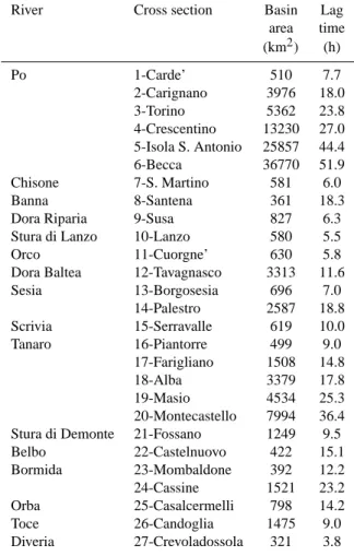
The model is calibrated on the base of the period 1999– 2001 and showed, on average, a good performance. The 27 cross sections considered cover almost all the main river net-work of the Po basin with a high variety of hydrological char-acteristics (Fig. 2 and Table 2).

To synthesize the hydrological model behaviour a relative error is calculated for each peak flood forecast either in terms of discharge (Eq. 1) and in terms of arrival time (Eq. 2). In the end, to account for the geomorphologic differences of each studied catchment, a normalized index which takes into account the advance of forecasts versus lag time is adopted (Eq. 3).

QDF error =Qf orecast−Qobserved

max (Qobserved)

(7)

Table 2. Characteristics of the studied catchments.

River Cross section Basin Lag

area time (km2) (h) Po 1-Carde’ 510 7.7 2-Carignano 3976 18.0 3-Torino 5362 23.8 4-Crescentino 13230 27.0 5-Isola S. Antonio 25857 44.4 6-Becca 36770 51.9 Chisone 7-S. Martino 581 6.0 Banna 8-Santena 361 18.3

Dora Riparia 9-Susa 827 6.3

Stura di Lanzo 10-Lanzo 580 5.5

Orco 11-Cuorgne’ 630 5.8

Dora Baltea 12-Tavagnasco 3313 11.6

Sesia 13-Borgosesia 696 7.0 14-Palestro 2587 18.8 Scrivia 15-Serravalle 619 10.0 Tanaro 16-Piantorre 499 9.0 17-Farigliano 1508 14.8 18-Alba 3379 17.8 19-Masio 4534 25.3 20-Montecastello 7994 36.4

Stura di Demonte 21-Fossano 1249 9.5

Belbo 22-Castelnuovo 422 15.1 Bormida 23-Mombaldone 392 12.2 24-Cassine 1521 23.2 Orba 25-Casalcermelli 798 14.2 Toce 26-Candoglia 1475 9.0 Diveria 27-Crevoladossola 321 3.8

T ime error =T (Qmax,f orecast) − T (Qmax,observed)

T c (2)

i a = T (Qmax,observed) − T OF

T c (3)

T (Qmax)is the time of the peak discharge (observed or

fore-casted), TOF is the time of forecast and Tc is the lag time of the basin obtained on the base of the SCS method (USDA, 1986). A sketch is given in Fig. 7 for Candoglia cross section along Toce river. Normalization is necessary to compare er-rors for the different catchments. As showed in Table 3 QDF error is generally negative, meaning an underestimation of the hydro-meteorological coupling. The “perfect forecast” shows the minimum mean error in both cases: this implies that generally the hydrological model itself has good perfor-mances; “S2” and “S4” have very similar behaviour with a slight degradation of the performance with respect to “Per-fect Forecast”; “S1” and “S3” show the worse behaviour with strong underestimation for the first event and overestimation for the second.

As far as the arrival time is concerned (Table 4) it can be noted that all forecasts show a peak arrival ahead of time while the hydrological model itself would produce a slight delay.

TOCE A CANDOGLIA - forecast time 15/11/2002 12:00 UTC

0 200 400 600 800 1000 1200 1400 1600 1800 15/11/2002 12:00 16/11/2002 12:00 17/11/2002 12:00 18/11/2002 12:00 19/11/2002 12:00 Forecast Observation

Peak discharge error Advance in forecast Peak time error

m3_/s

Figure 7. Comparison between forecasted and observed hydrograph

23 Fig. 7. Comparison between forecasted and observed hydrograph.

Hydrological forecast errors versus the forecast advance index is shown in Fig. 8. It seems clear that the underesti-mation is not strictly linked to the advance of forecast and this is in contrast with what we are usually confident in. This highlights the heavy role of the uncertainties linked to mete-orological forecasts even for short horizons.

4 The hydro-meteorological chain

From an operational point of view, the error analysis in terms of forecasted discharge it’s not satisfactory. It is very impor-tant to understand how these errors impact on the reliability of the alert system. The objective is to understand the rela-tive weight of these sources of uncertainty in flood warning procedures reliability.

For each cross section, a dangerous floods level is defined on the base of discharge thresholds that are evaluated by means of off-line hydraulic analysis of each river reach and, when available, considering historical floods data. In this way, the QDFs allow the definition of the expected risk level looking at the expected flood peak along with the discharge threshold.

Comparing observed and forecasted threshold overcoming for all the cross sections produce false and failed alarms. Or-ganising this results in a classical contingency table one can use the Statistical indices (TS, BIAS), to point out the be-haviour of the alert system during the events (Table 5). The results obtained using the whole hydro-meteorological chain offer a basis to evaluate its sensitivity to the uncertainties in the numerical simulations related to the performance of the alert system.

As it can be noticed the response is not very good: “Perfect forecast” results highlight that the flood warning in little and medium sized catchments is far to be reliable even from the hydrological point of view with several missed alarms. Forc-ing the model with meteorological inputs makes the system behave in a very unstable way producing even worse results.

(8)

(a) S1 0 1 2 3 4 5 6 7 8 9 10 11 -2 -1 0 1 2 3 4 5 6 7 QDF relative error (%) advance ti me i ndex S2 0 1 2 3 4 5 6 7 8 9 10 11 -2 -1 0 1 2 3 4 5 6 7 QDF relative error (%) advance ti me i ndex S3 0 1 2 3 4 5 6 7 8 9 10 11 -2 -1 0 1 2 3 4 5 6 7 QDF relative error (%) advance ti me i ndex S4 0 1 2 3 4 5 6 7 8 9 10 11 -2 -1 0 1 2 3 4 5 6 7 QDF relative error (%) advance ti me i ndex

Figure 8. Peak discharge forecast relative error versus advance time index

24

(b) S1 0 1 2 3 4 5 6 7 8 9 10 11 -2 -1 0 1 2 3 4 5 6 7 QDF relative error (%) advance ti me i ndex S2 0 1 2 3 4 5 6 7 8 9 10 11 -2 -1 0 1 2 3 4 5 6 7 QDF relative error (%) advance ti me i ndex S3 0 1 2 3 4 5 6 7 8 9 10 11 -2 -1 0 1 2 3 4 5 6 7 QDF relative error (%) advance ti me i ndex S4 0 1 2 3 4 5 6 7 8 9 10 11 -2 -1 0 1 2 3 4 5 6 7 QDF relative error (%) advance ti me i ndex

Figure 8. Peak discharge forecast relative error versus advance time index

24

(c) S1 0 1 2 3 4 5 6 7 8 9 10 11 -2 -1 0 1 2 3 4 5 6 7 QDF relative error (%) advance ti me i ndex S2 0 1 2 3 4 5 6 7 8 9 10 11 -2 -1 0 1 2 3 4 5 6 7 QDF relative error (%) advance ti me i ndex S3 0 1 2 3 4 5 6 7 8 9 10 11 -2 -1 0 1 2 3 4 5 6 7 QDF relative error (%) advance ti me i ndex S4 0 1 2 3 4 5 6 7 8 9 10 11 -2 -1 0 1 2 3 4 5 6 7 QDF relative error (%) advance ti me i ndex

Figure 8. Peak discharge forecast relative error versus advance time index

24

(d) S1 0 1 2 3 4 5 6 7 8 9 10 11 -2 -1 0 1 2 3 4 5 6 7 QDF relative error (%) advance ti me i ndex S2 0 1 2 3 4 5 6 7 8 9 10 11 -2 -1 0 1 2 3 4 5 6 7 QDF relative error (%) advance ti me i ndex S3 0 1 2 3 4 5 6 7 8 9 10 11 -2 -1 0 1 2 3 4 5 6 7 QDF relative error (%) advance ti me i ndex S4 0 1 2 3 4 5 6 7 8 9 10 11 -2 -1 0 1 2 3 4 5 6 7 QDF relative error (%) advance ti me i ndex

Figure 8. Peak discharge forecast relative error versus advance time index

24

Fig. 8. Peak discharge forecast relative error versus advance time index.

Table 3. Synthesis of relative errors for peak discharge forecast.

Case study: ITALIA1 Case study: ITALIA2

QPF model Mean error Standard deviation Mean error Standard deviation

Perfect forecast −0.08 0.59 −0.07 0.38

S1 −0.48 0.66 0.21 0.99

S2 −0.26 1.26 −0.09 0.52

S3 −0.46 0.78 0.22 0.96

S4 −0.29 1.26 −0.16 0.44

Table 4. Synthesis of relative errors for peak time forecast.

Case study: ITALIA1 Case study: ITALIA2

QPF model Mean error Standard deviation Mean error Standard deviation

Perfect forecast 0.13 0.56 0.19 0.88 S1 −0.63 1.32 −1.22 1.59 S2 −0.93 1.43 −0.52 1.81 S3 −0.54 1.29 −1.15 1.50 S4 −0.82 1.31 −0.76 1.92 5 Conclusion

The results of meteorological activities prove that initial and boundary conditions are important sources of error in the forecast as far as very complex orography is involved. On the contrary, the dependency on the domain of integration is weak, at least for these test cases. Globally runs derived from ECMWF better reproduce the rainfall fields.

It is confirmed that forcing hydrological forecast over little and medium sized catchments with global model QPFs pro-duces significant errors. Furthermore, when considering the little and medium sized watersheds, the hydrological model itself shows important uncertainties due to the initial condi-tion and to the simplified physical processes.

An important feature here noticed is linked to the compar-ison between meteorological and hydrological model

(9)

perfor-852 D. Rabuffetti and M. Milelli: The hydro-meteorological chain in Piemonte

Table 5. Warning system performance.

Case study ITALIA1 ITALIA2

Model TS BIAS TS BIAS

Perfect forecast 0.14 0.20 0.38 0.38

S1 0.15 0.15 0.00 0.80

S2 0.10 0.15 0.20 0.20

S3 0.15 0.15 0.00 0.38

S4 0.05 0.05 0.13 0.13

mance evaluation. In terms of 48 h average rainfall over the areas, statistical indices show quite good results. Anyway, when the forecasts are used to force the hydrological simula-tion, these errors becomes greater enhancing the well known problem of the different space time scales typical of the two different domains.

All the uncertainties present in the hydro-meteorological chain cause significant errors in terms of discharge forecast-ing. Of course, this impacts on the alert system performance but, at least for these test cases, the reliability of the whole warning system is not strictly related to the magnitude of those errors. In this study for example, little or heavy un-derestimation of peak discharge, due respectively to “perfect forecast” runs and meteorological forecast driven runs, can produce a similar number of missed alarms. At the same time, the importance and the need of a human intervention of expert hydrologists in analysing model runs and results is here highlighted.

Acknowledgements. This work was funded in the framework of

HYDROPTIMET 2002-02-4.3-I-084 “Optimisation des outils de prévision Hydrométéorologique”, EU-INTERREG IIIB MEDOCC. Edited by: R. Romero

Reviewed by: two referees

References

Barbero, S., Rabuffetti, D., Wilson, G., and Buffo, M.: Develop-ment of a Physically-Based Flood Forecasting System: “MIKE FloodWatch” in the Piemonte Region, Italy, proc. 4th DHI Soft-ware Conference, Helsingør, Denmark, 2001.

Cressman, G. P.: An operational objective analysis system. Mon. Wea. Rev., 87, 367–374, 1959.

COSMO Newsletter No. 5: Deutscher Wetterdienst, Offenbach am Main, 2005.

Doms, G., Foerstner, J., Heise, E., Herzog, H.-J., Raschendorfer, M., Schrodin, R., Reinhardt, T., and Vogel, G.: A description of the non-hydrostatic regional model LM. Part II: physical param-eterisation, available at http://www.cosmo-model.org, 2005. Ferraris, L., Rudari, R., and Siccardi, F.: The uncertainty in the

prediction of flash floods in the northern Mediterranean environ-ment, J. Hydrometeorology, 3, 714–727, 2002.

Jasper, K. and Kaufmann P.: Coupled runoff simulations as valida-tion tools for atmospheric models at the regional scale, Quart. J. Roy. Meteorl. Soc., 129B, no. 588, 2003.

Krzysztofowicz, R.: Bayesian theory of probabilistic forecvast-ing via deterministic hydrologic model, Water Resour. Res., 35, 2739–2750, 1999.

Milelli, M., Oberto, E., Bertolotto, P., and Pelosini, R.: Verification of QPF over Piemonte and northern Italy using high-resolution non-GTS data, Proc. of the ECAM/EMS Annual Meeting, Rome, Italy, September, 2003.

Murphy, A. H. and Winkler, R. L.: A general framework for forecast verification, Monthly Weather Review, 115, 1330–1338, 1997. Parker, D. J. and Fordham, M.: An evaluation of flood forecasting,

warning and response systems in the European Union, Water Re-sources Management, 10, 279–302, 1996.

Romero, R.: Climatological and meteorological aspects of West-ern Mediterranean cyclones: impacts on precipitation, Geophys. Res. Abst., 6, 2004,

SRef-ID: 1607-7962/gra/EGU04-A-07724.

Schraff, C. and Hess, R.: A description of the non-hydrostatic re-gional model LM, Part III: data assimilation, available at http: //www.cosmo-model.org, 2003.

Torrisi, L.: Impact of domain size on LM forecast, COSMO Newsletter No. 5, available at http://www.cosmo-model.org, 2005.

USDA: US Department of Agriculture, Soil Conservation Service, National Engineering Handbook, section 4, Hydrology, Rev. ed., US Department of Agriculture, 1972 and 1986.

Wilks, D.: Statistical Methods in the Atmospheric Sciences, Aca-demic Press, 1995.