HAL Id: hal-00297915
https://hal.archives-ouvertes.fr/hal-00297915
Submitted on 27 Aug 2007HAL is a multi-disciplinary open access
archive for the deposit and dissemination of sci-entific research documents, whether they are pub-lished or not. The documents may come from teaching and research institutions in France or abroad, or from public or private research centers.
L’archive ouverte pluridisciplinaire HAL, est destinée au dépôt et à la diffusion de documents scientifiques de niveau recherche, publiés ou non, émanant des établissements d’enseignement et de recherche français ou étrangers, des laboratoires publics ou privés.
Inorganic carbon time series at Ocean Weather Station
M in the Norwegian Sea
I. Skjelvan, E. Falck, F. Rey, S. B. Kringstad
To cite this version:
I. Skjelvan, E. Falck, F. Rey, S. B. Kringstad. Inorganic carbon time series at Ocean Weather Station M in the Norwegian Sea. Biogeosciences Discussions, European Geosciences Union, 2007, 4 (4), pp.2929-2958. �hal-00297915�
BGD
4, 2929–2958, 2007 Inorganic carbon time series I. Skjelvan et al. Title Page Abstract Introduction Conclusions References Tables Figures ◭ ◮ ◭ ◮ Back CloseFull Screen / Esc
Printer-friendly Version Interactive Discussion
EGU
Biogeosciences Discuss., 4, 2929–2958, 2007 www.biogeosciences-discuss.net/4/2929/2007/ © Author(s) 2007. This work is licensed
under a Creative Commons License.
Biogeosciences Discussions
Biogeosciences Discussions is the access reviewed discussion forum of Biogeosciences
Inorganic carbon time series at Ocean
Weather Station M in the Norwegian Sea
I. Skjelvan1,2, E. Falck2, F. Rey3, and S. B. Kringstad2,1
1
Bjerknes Centre for Climate Research, University of Bergen, Norway
2
Geophysical Institute, University of Bergen, Norway
3
Institute of Marine Research, Bergen, Norway
Received: 15 August 2007 – Accepted: 23 August 2007 – Published: 27 August 2007 Correspondence to: I. Skjelvan (ingunn.skjelvan@gfi.uib.no)
BGD
4, 2929–2958, 2007 Inorganic carbon time series I. Skjelvan et al. Title Page Abstract Introduction Conclusions References Tables Figures ◭ ◮ ◭ ◮ Back CloseFull Screen / Esc
Printer-friendly Version Interactive Discussion
EGU
Abstract
Dissolved inorganic carbon (CT) has been collected at Ocean Weather Station M
(OWSM) in the Norwegian Sea since 2001. Seasonal variations in CT are confined
to the upper 50 m, where the biology is active, and below this layer no clear seasonal signal is seen. From winter to summer the surface CT concentration typical drops
5
from 2140 to about 2040 µmol kg−1, while a deep water CT concentration of about
2163 µmol kg−1 is measured throughout the year. Observations show an annual in-crease in salinity normalized carbon concentration (nCT) of 1.3±0.7 µmol kg−1 in the
surface layer, which is equivalent to a pCO2 increase of 2.6±1.2 µatm yr−1, i.e. larger
than the atmospheric increase in this area. Observations also show an annual increase
10
in the deep water nCT of 0.57±0.24 µmol kg−1, of which about a tenth is due to inflow of
old Arctic water with larger amounts of remineralised matter. The remaining part has an anthropogenic origin and sources for this might be Greenland Sea surface water, Ice-land Sea surface water, and/or recirculated Atlantic Water. By using an extended multi linear regression method (eMLR) it is verified that anthropogenic carbon has entered
15
the whole water column at OWSM.
1 Introduction
The ocean is one of several reservoirs indirectly controlling the climate system through exchange of CO2 with the atmosphere. Human activities, such as burning of fossil
fuels and deforestation, release annually an anthropogenic carbon amount of about
20
7.2×10¹⁵g C into the atmosphere, and of this, about one third is taken up by the world oceans (IPCC, 2007). The North Atlantic is known to store relatively large amounts of anthropogenic carbon, which has been captured through formation of intermediate and deep waters in subpolar areas (Friis et al., 2005). It is, however, not straight forward to quantify this amount, due to a lack of oceanic reference data from the pre-industrial
25
BGD
4, 2929–2958, 2007 Inorganic carbon time series I. Skjelvan et al. Title Page Abstract Introduction Conclusions References Tables Figures ◭ ◮ ◭ ◮ Back CloseFull Screen / Esc
Printer-friendly Version Interactive Discussion
EGU
In particular, the Nordic Seas in the northern North Atlantic is described as an im-portant sink region for atmospheric CO2 (e.g. Takahashi et al., 2002; Skjelvan et al.,
2005), however, recent research suggests that the size of this sink seems to be region-ally decreasing, based on an observed seawater fCO2which annually increases faster than the atmospheric fCO2(Olsen et al., 2006). Carbon time series data from this area
5
are, in this respect, valuable contributions to evaluate the development of the oceanic carbon uptake.
The Ocean Weather Station M (OWSM) is situated in the western branch of the Nor-wegian Atlantic Current, at 66◦N; 2◦E, over the Norwegian continental slope (Fig. 1). The station, which has a depth of about 2100 m, was started in 1948 and is today
op-10
erated by M/S Polarfront; the last weather ship in the world. Temperature and salinity have been measured from the very beginning (e.g. Østerhus and Gammelsrød, 1999; Nilsen and Falck, 2006), closely followed by dissolved oxygen (Nilsen and Falck, 2006; Kivim ¨ae and Falck, 20071). In the 1980s analyses of atmospheric CO2 content were started (Tans and Conway, 2005), and since 1990 nutrients have been determined
15
weekly (Dale et al., 1999). During a four years period and on a monthly basis in the early 1990s, total dissolved inorganic carbon (CT) was determined for the very first time at OWSM, using gas extraction of acidified water samples and manometric detection (Gislefoss et al., 1998), however, these are not used in the following due to insufficient precision (±12 µmol kg−1). Since November 2001 monthly measurements of C
T and
20
alkalinity has been performed using modern analyzing techniques.
Warm and saline Atlantic Water from the Norwegian Atlantic Current occupies the upper layer at OWSM down to 300–400 m, with present temperatures typically varying between 7◦C in the winter and 12◦C in the summer time. Cold and less saline deep water occupies the water column from about 1000 m down to the bottom (Norwegian
25
Sea Deep Water), and in between these two water masses there is a layer of interme-1
Kivim ¨ae, C. and Falck, E.: Interannual variability of net community production at Ocean Weather Station M in the Norwegian Sea during 51 years, Global Biogeochem. Cycles, sub-mitted, 2007.
BGD
4, 2929–2958, 2007 Inorganic carbon time series I. Skjelvan et al. Title Page Abstract Introduction Conclusions References Tables Figures ◭ ◮ ◭ ◮ Back CloseFull Screen / Esc
Printer-friendly Version Interactive Discussion
EGU
diate water; Arctic Intermediate Water, of fluctuating thickness. At times with northerly or north-easterly winds during summer, the fresher Norwegian Coastal Water is driven away from the coast and will occasionally reach all the way out to OWSM. We refer to Nilsen and Falck (2006) for a more thorough description of the hydrographic conditions in the OWSM area.
5
In this paper we present the new CT time series data from OWSM in the Norwegian
Sea since fall 2001. We describe the seasonal and interannual variations, and we use the multiple linear regression (MLR) method of Wallace (1995) in an extended version formalized by Friis et al. (2005); eMLR; to determine the anthropogenic CO2increase
in this area of the Nordic Seas during the last two decades since the Transient Tracers
10
in the Ocean, North Atlantic Study (TTO-NAS) expedition in 1981.
2 Data
At present, hydrographic measurements at OWSM are performed using a Sea-Bird CTD (SBE 37-SM MicroCAT with conductivity, temperature, and pressure sensors), which is calibrated towards bottle salinity samples. Nansen bottles, with reversing
15
thermometers, are used to collect samples for inorganic carbon, dissolved oxygen, nutrients, and salinity at standard depths. Samples for CT are conserved with 0.02%, by volume, of saturated HgCl2solution and analysed ashore in general within a month,
however, a few samples have been stored for up to six months when the analytical instruments have been occupied at cruises. CT is determined by gas extraction of
20
acidified water samples and further coulometric titration (DOE, 1994; Johnson et al., 1993), and accuracy is set by running CRM supplied by Andrew Dickson of Scripps Institution of Oceanography. The precision has been determined to ±0.5 µmol kg−1
based on 10 duplicate samples. A comparison of the Norwegian Sea Deep Water, year by year, resulted in a standard deviation of ±1.5 µmol kg−1; however, this most
25
likely has other sources than imprecision in the measurements. Dissolved oxygen is measured on board using the Winkler titration method with visual detection of the
BGD
4, 2929–2958, 2007 Inorganic carbon time series I. Skjelvan et al. Title Page Abstract Introduction Conclusions References Tables Figures ◭ ◮ ◭ ◮ Back CloseFull Screen / Esc
Printer-friendly Version Interactive Discussion
EGU
titration end point, and this in general gives a precision of 1%. Nutrients are conserved using chloroform and kept at 4◦C until analysis ashore within six weeks after sampling.
The analyses were made using standard methods on a Skalar Auto Analyzer until 2003 and an Alpkem Auto Analyzer since then. Precision for nitrate, phosphate, and silicate are 3%, 4%, and 2%, respectively. The salinity samples are analyzed ashore within
5
a month after sampling using PorterSal salinometer with a precision of 0.003. Due to technical problems there is a gap in the time series from April to October 2004, i.e. no water samples were collected during this period.
The TTO-NAS ran from April to October 1981 and consisted of 7 legs. In the present study we have used data from leg 5, which was carried out during July and August 1981
10
in the Nordic Seas, and the precision of these data is reported to be ±3.7 µmol kg−1.
The data are obtained from the Carbon Dioxide Information Analysis Center (Oak Ridge, Tennessee, USA) and are thoroughly described in e.g. Olsen et al. (2006). Tanhua and Wallace (2005) reanalyzed TTO data from legs 2, 3, 4, and 7, and com-pared them with modern data adjusted to CRMs. Based on this they recommended
15
that the TTO alkalinity data should be reduced by 3.4 µmol kg−1, and that the TTO CT data should be recalculated using adjusted alkalinity data and further increased by 2.4 µmol kg−1. This correction has also been performed on the data from leg 5.
3 Seasonal and interannual variability
The inorganic carbon content of the seawater in this area varies at different time scales.
20
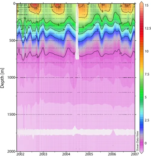
The upper water mass at OWSM experiences seasonal changes due to physical, chemical, and biological processes. A clear seasonality is, for instance, seen in the upper layer temperature with warming during the summer seasons and cooling during winters (Fig. 2). The depth of the mixed layer at OWSM varies in general between 20 m in summer to 300–400 m in winter (Nilsen and Falck, 2006) and below the winter
25
mixed layer no clear seasonal signal is seen (Fig. 2). However, the depth of the tran-sition layer between the Atlantic Water and the intermediate water at OWSM is known
BGD
4, 2929–2958, 2007 Inorganic carbon time series I. Skjelvan et al. Title Page Abstract Introduction Conclusions References Tables Figures ◭ ◮ ◭ ◮ Back CloseFull Screen / Esc
Printer-friendly Version Interactive Discussion
EGU
to fluctuate considerably (e.g. Mosby, 1962) and this can clearly be seen in Fig. 2 at depths between 300 and 600 m, where the period of the temperature fluctuations is disconnected with the season. Below about 700 m the temperature decreases toward the bottom from 0 to about –0.83◦C.
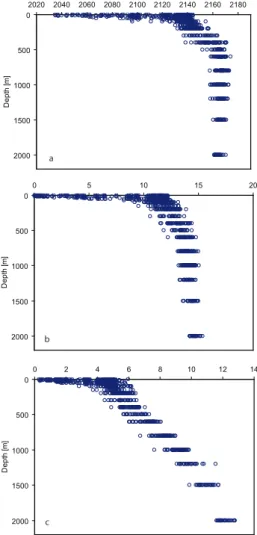
Figure 3 shows all the CT, nitrate, and silicate data from 2001 to 2006, and Fig. 4
5
shows CT, nitrate, silicate, temperature, and salinity at different depth layers from 2001
to 2006. The highest variability for all parameters is seen in the surface layer, and this is closely linked to the biological activity starting in the spring and extending into the summer season. The phytoplankton growth starts in April-May as a combined result of increased solar radiation, shallowing of the mixed layer, and the establishment of a
10
seasonal pycnocline (Rey, 2004). With the onset of the primary production the con-centrations of CT and nutrients decrease in the surface layer. This depletion continues
until mid or late summer, when respiration and remineralisation take over as dominating processes controlling the CT and nutrients concentrations.
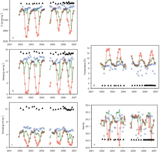
At 50 m depth there is a temporary decrease in CT, nitrate, and silicate
concentra-15
tions just after the onset of primary production, when the mixed layer is still deeper than 50 m. The major depletion at this depth appears to occur in September-October (Figs. 4a, b, and c), when the surface water low in CT and nutrients is mixed downwards
due to wind mixing and vertical convection achieved by cooling of the surface (Fig. 4d). As the mixed layer depth increases further the carbon and nutrient rich waters from
20
depths below 50 m are mixed upwards in the water column and reintroduced into the surface layer, increasing the surface concentrations towards winter values.
The biological drawdown during spring and summer is confined to the upper 50 m and below 100 m there is no clear seasonal signal in CT and nutrients. From winter to
summer the surface CT, nitrate, and silicate decrease by about 100, 11, and 4 µmol
25
kg−1, respectively (Figs. 4a, b, and c). The lowest CT concentrations are found in
August, while the nutrients have their lowest concentrations in July.
While there is an indisputable difference between summer and winter values in upper waters, no clear seasonal signal is seen in the deeper layers. In the transition zone
BGD
4, 2929–2958, 2007 Inorganic carbon time series I. Skjelvan et al. Title Page Abstract Introduction Conclusions References Tables Figures ◭ ◮ ◭ ◮ Back CloseFull Screen / Esc
Printer-friendly Version Interactive Discussion
EGU
between the Atlantic Water and the Arctic Intermediate Water (300–600 m; Fig. 3a) the CT concentration increases from about 2140 to about 2165 µmol kg−1. In the core of
the intermediate water, between about 500 and 1000 m, there is a small CT maximum
(Fig. 3a), and below this the concentration is slightly decreasing towards the bottom. For nitrate (Fig. 3b), the increase in the transition layer is 2 µmol kg−1, with a small
5
further increase of 1 µmol kg−1 in the deep water. The silicate concentration (Fig. 3c) increases from about 6 to about 9 µmol kg−1 in the transition zone, and increases further towards the bottom. At 2000 m depth CT, nitrate, and silicate values are about 2163, 15, and 12 µmol kg−1, respectively, throughout the year. Typical values for the different parameters at different depth layers and seasons are presented in Table 1,
10
however, deviations from these are certainly observed.
When it comes to interannual variations, the degree of carbon depletion in the mixed layer during summer seasons do vary from year to year; a feature which is also seen in the silicate, but not in the nitrate (Figs. 4a, b, and c). During 2005 the concentration of CT dropped by about 80 µmol kg−1 from winter to summer compared to a CT drop
15
of about 100 µmol kg−1 from winter to summer in previous years. A similar picture is seen for the salinity normalized CT (nCT=CT·S/35.1; not shown), which indicates that
this feature is not caused by a change in salinity. The feature is mainly explained by a colder surface temperature during summer 2005 compared to the previous summers (see Figs. 2 and 4d). During 2005 the surface temperature was about 2◦C colder
20
than previous years, and this corresponds to a CT increase of about 16 µmol kg−1
(Lewis and Wallace, 1998). Also surface silicate values were less depleted during summer 2005 and 2006 compared to previous summers. The reason for this might be connected to sub-optimal diatom growth or to heavy grazing on diatoms resulting in a lower phytoplankton biomass (Rey, 2004).
25
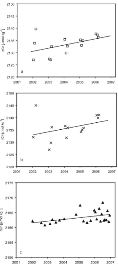
To determine any interannual trend in the inorganic carbon content of the surface water the winter surface (10 m) nCT concentration during the years 2002 to 2006 is plotted in Fig. 5a. Winter season is defined as the months January to March, and a re-gression line is drawn through the points. The figure shows two things; first, within the
BGD
4, 2929–2958, 2007 Inorganic carbon time series I. Skjelvan et al. Title Page Abstract Introduction Conclusions References Tables Figures ◭ ◮ ◭ ◮ Back CloseFull Screen / Esc
Printer-friendly Version Interactive Discussion
EGU
same winter the mixed layer in general increases from January towards March, which increases the carbon concentration in the surface layer. Second, and most interesting when it comes to variations from year to year, the slope of the regression line indicates an annual nCT increase of 1.3±0.7 µmol kg−1 (with a significance level of 92%). An
annual increase of not salinity normalized CT values of 1.5±0.5 µmol kg−1 was also
5
determined (not shown), which indicates that less than a tenth of the observed annual increase in surface CT is due to salinity changes. The slope in nCT is equivalent to
a pCO2 increase of 2.6±1.2 µatm yr−1 (at constant alkalinity of 2320 µmol kg−1; Lewis
and Wallace, 1998). The winter season was chosen to eliminate any interannual varia-tions in primary production. To check the solidity in this interannual signal we examined
10
the carbon content in the winter (January to March) mixed layer over the years, since the winter is the time of the year when the mixed layer is deepest and coldest (Nilsen and Falck, 2006). The mixed layer depth was determined as the depth where the σt
had changed equivalent to a decrease in the surface temperature of 0.8◦C (Kara et al., 2000). For density profiles with surface instability stronger than 0.02 kg m−3 the first
15
stable value below the surface was used as the surface value. Further, the averaged salinity normalized carbon content of the mixed layer during the winter months were calculated by integrating over the mixed layer, and the result is plotted in Fig. 5b. The slope of the regression line indicates an increase in the mixed layer carbon content of 1.2±0.9 µmol kg−1yr−1 (equivalent to an annual pCO2 increase of 2.4±1.6 µatm;
20
Lewis and Wallace, 1998), which is similar to what is determined for the surface water. According to Tans and Conway (2005) and T. Conway (personal communication) the annual atmospheric CO2increase at OWSM was 2.1±0.2 µatm for the period between
2001 and 2005, and 1.63±0.03 µatm for the period between 1982 to 2005; i.e. less compared to the oceanic carbon increase.
25
A closer look into the deep water CT (Fig. 5c) also shows an interannual signal, and
at 2000 m deep the nCT increases by 0.57±0.24 µmol kg−1 yr−1 (significance level of 97%). This might be connected to the changes seen in the deep water at OWSM during the last decades (Østerhus and Gammelsrød, 1999) and will be discussed further in
BGD
4, 2929–2958, 2007 Inorganic carbon time series I. Skjelvan et al. Title Page Abstract Introduction Conclusions References Tables Figures ◭ ◮ ◭ ◮ Back CloseFull Screen / Esc
Printer-friendly Version Interactive Discussion
EGU
Chapter 5. At 800, 1000, and 1500 m we observe annual increases in nCT of 1.4, 0.8 and 0.9 µmol kg−1, respectively.
4 Determining changes in anthropogenic carbon
During the last decade or so there have been numerous attempts to determine the anthropogenic part of the carbon exchange between the atmosphere and the ocean
5
(e.g. Wallace, 1995; Gruber et al., 1996; Sabine et al., 1999). In this work we have used the extended multi linear regression (eMLR) method documented in Friis et al. (2005), which has its origin in the multivariate time-series method of Wallace (1995), to deter-mine changes in the anthropogenic carbon content of the water.
The method is based upon the assumptions that the spatial CT distribution in a given
10
region can be described by a linear multi-parameter model and that, over the time period of the study, there are no temporal changes in the correlation between CT and
the independent parameters used in the method. In the real world, CT is perturbed both
by natural variability and anthropogenic input, but it is assumed that when predictive parameters like salinity, nutrients, AOU (apparent oxygen utilization), or alkalinity are
15
taken into account this can adjust for the natural variations.
The rationale is to use a recent data set from one region; in this case OWSM data from 2005, and compare it with a historical data set from the same region; i.e. data from the TTO-NAS expedition in 1981. CT values from the two time periods are predicted by
using a combination of independent parameters; salinity, nitrate, silicate, and potential
20
temperature, from the respective time periods:
CT ,predt = at+ btSt+ ctNOt3+ dtSiOt2+ etθt (1) where a, b, c, d , and e are regression coefficients specific for the particular dataset, and t refers to the TTO or OWSM data. The change of anthropogenic carbon in the water column over the time span is then determined by subtracting the time specific
BGD
4, 2929–2958, 2007 Inorganic carbon time series I. Skjelvan et al. Title Page Abstract Introduction Conclusions References Tables Figures ◭ ◮ ◭ ◮ Back CloseFull Screen / Esc
Printer-friendly Version Interactive Discussion
EGU
equations from each other: ∆CTant= (a
t2
− at1) +(bt2− bt1)St2+(ct2− ct1)NO3t2+(dt2− dt1)Si Ot22 +(et2− et1)θt2(2) where t1 and t2 represents the TTO and OWSM data, respectively. A similar approach is used in Olsen et al. (2006). An advantage of the eMLR approach compared to the MLR is that the measurement error of the independent parameters is minimized since
5
this error is included in the prediction both in the recent and the historical dataset (Friis et al., 2005).
With the view of the Norwegian Sea as a diatom dominated area, it makes sense that silicate is one of the parameters that should be included in the predictive term for CT. On the other hand, parameters like phosphate and AOU were also considered in
10
the regression, with not as good fit as with the present combination of parameters. The use of phosphate and AOU even resulted in CT residuals with a biased variation with
depth, which indicates that these parameters are not independent.
From the TTO-NAS, Leg 5, we have chosen 3 stations from the Nordic Seas (see Fig. 1). These data were chosen due to relatively similar hydrographical characteristics
15
to those found at OWSM (see Fig. 6). Nitrate values lower than 0.5 µmol kg−1, which were the case for a few data points, have been excluded in both datasets to avoid situations with possible overconsumption of carbon at low nutrient levels (Falck and Anderson, 2005). The eMLR approach was applied and Table 2 presents essential outputs from the calculation, such as regression coefficients of Eq. (1) for the TTO and
20
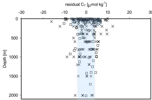
OWSM data and statistics. The calculated CT residuals (CTmeasured–CTpredicted) from
the two datasets were relatively homogenously distributed around zero throughout the water column (Fig. 7), which support the choice of independent variables for the CT prediction. The highest scatter is found in the surface layer, which is the area of high biological activity, and this expresses that the method does not fully compensate for
25
the biology. The distribution of the CT residuals is used to estimate the accuracy of the eMLR method, and for the upper 200 m the accuracy is set to ±7 µmol kg−1, while
BGD
4, 2929–2958, 2007 Inorganic carbon time series I. Skjelvan et al. Title Page Abstract Introduction Conclusions References Tables Figures ◭ ◮ ◭ ◮ Back CloseFull Screen / Esc
Printer-friendly Version Interactive Discussion
EGU
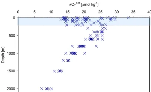
Fig. 8 presents the anthropogenic increase of carbon at OWSM in the Norwegian Sea over the 24 years period from 1981 to 2005. The variation in the surface layer is large; however, the overall picture is that anthropogenic carbon seems to have entered the whole water column during these 24 years. The deep layer has experienced the lowest anthropogenic carbon increase of about 9±4 µmol kg−1 and the upper water
5
mass has increased its anthropogenic carbon content of about 25±7 µmol kg−1. Olsen et al. (2006) calculated increases in anthropogenic carbon of the surface and deep waters of about 17±10 and 6±5 µmol kg−1, respectively, over 21.5 years at a location west of OWSM. The present study indicates that the anthropogenic carbon input might have been slightly larger than this.
10
The eMLR method was checked by using Eq. (2) to backward calculate the ∆CantT ,
i.e. regression constants for TTO data subtracted from regression constants for OWSM data and further multiplied with TTO data. This showed an anthropogenic carbon in-crease similar to Fig. 8, which confirms the solidity of the eMLR method.
OWSM data from 2006 were also tried out in the anthropogenic carbon change
cal-15
culation, but due to some strange surface water results these data were not used fur-ther in the eMLR calculations.
5 Discussion
Until recently, the oceanic uptake of atmospheric CO2at high latitudes has been sup-posed to be increasing due to a strong deep mixing (Takahashi et al., 2002). The
argu-20
ment has been that under such mixing conditions any oceanic signal of the increasing atmospheric CO2 content would be diluted to undetectable levels, i.e. the ocean
sur-face would not show any detectable interannual increase of pCO2. In the current study, which focuses on OWSM in the Norwegian Sea, the surface water carbon content is observed to increase at a slightly higher speed (2.6 µatm yr−1) than what is seen in
25
the atmosphere (2.1 µatm yr−1) over the years 2001 to 2006, which is in concert with
BGD
4, 2929–2958, 2007 Inorganic carbon time series I. Skjelvan et al. Title Page Abstract Introduction Conclusions References Tables Figures ◭ ◮ ◭ ◮ Back CloseFull Screen / Esc
Printer-friendly Version Interactive Discussion
EGU
The consequence of this is that the oceanic uptake of atmospheric CO2in this area is decreasing and the carbon content of the Atlantic Water seems to be moving towards equilibrium with respect to air-sea CO2exchange; i.e. no net oceanic uptake or release
of CO2. This is intuitively in contradiction to an atmosphere with an increasing amount of CO2. However, according to Wallace (2001) this can be explained by a reduction in
5
the buffer capacity of the northward flowing water compared to previous times. This is a result of a reduced out-gassing at lower latitudes due to higher atmospheric CO2levels. In this way more carbon is left in the water to be transported northwards, and when the water cools on its way towards the Nordic Seas less atmospheric carbon, compared to pre-industrial times, is absorbed in the water in order to maintain equilibrium with the
10
atmosphere. This is also verified by Anderson and Olsen (2002), who showed, using a simple advective model, that lower latitudes have the largest uptake of anthropogenic CO2 from the atmosphere, while higher latitudes have a smaller uptake or even are a
source of anthropogenic CO2 to the atmosphere. Olsen et al. (2006) used calculated pCO2 and measured δ
13
C values to determine the history of the Atlantic Water; the
15
water masses advected into the Nordic Seas have been exposed to an atmosphere elevated in CO2 for a long time and are therefore close to saturated with respect to CO2, hence there will be no further uptake of atmospheric carbon, which is in line with
the explanation of Wallace (2001).
The increase in surface carbon over the years at OWSM of about 1.3 µmol kg−1yr−1
20
(both observed and calculated from salinity normalized carbon concentration in the mixed layer) is also verified by the estimates of anthropogenic carbon increase using the eMLR method. The anthropogenic increase of the mixed layer (excluding the sur-face water) is estimated to be about 25 µmol kg−1 during a period of 24 years (Fig. 8), which equals an annual increase in mixed layer CT of about 1 µmol kg−1. From this it
25
seems that the eMLR method, in spite of the large standard deviation, is describing a situation close to the real world for the water in the mixed layer.
For the OWSM deep water, a carbon increase of 0.57±0.24 µmol kg−1yr−1 is ob-served based on data from 2001 to 2006. This increase might be due to both natural
BGD
4, 2929–2958, 2007 Inorganic carbon time series I. Skjelvan et al. Title Page Abstract Introduction Conclusions References Tables Figures ◭ ◮ ◭ ◮ Back CloseFull Screen / Esc
Printer-friendly Version Interactive Discussion
EGU
and anthropogenic effects. The question might rise if this CT increase is a
tempera-ture effect. To achieve a temperatempera-ture induced annual increase in the deep water CT
of 0.57 µmol kg−1, the deep water temperature must have decreased by about 0.06◦C each year. In contrast to this, Østerhus and Gammelsrød (1999) showed that the tem-perature of the Norwegian Sea Deep Water increased by about 0.1◦C from 1987 to
5
1998 and during the period of the present study the temperature has increased by about 0.004◦C per year, which eliminate the deep water CT increase as a temperature
effect.
So where does the increase in the Norwegian Sea Deep Water CT has its origin?
The increase must have been brought there by deep or intermediate currents, since
10
there is no deep convection in the Norwegian Sea. The general assumption is that the deep basin of the Norwegian Sea is fed by a mixture of deep water from the Green-land Sea, which traditionally has been colder and fresher than the deep water of the Norwegian Sea, and Arctic Ocean Deep Water, which has been warmer and saltier compared to the Greenland Sea Deep Water (e.g. Swift and Koltermann, 1988).
Dur-15
ing the 1980s the deep convection in the Greenland Sea slowed down considerably in the sense that the convection was not as deep as previously and only reached in-termediate depths (Schlosser et al., 1991). This induced a change in the exchange between the deep basins in the Arctic and Nordic Seas. The older Arctic Ocean Deep Water is lower in dissolved oxygen and higher in carbon and nutrients compared to
20
younger Greenland Sea Deep Water due to more time for remineralisation of organic matter to occur. Blindheim and Rey (2004) compared dissolved oxygen and silicate data from the Greenland Sea Deep Water during the period from 1980s to 2000 and found the oxygen and silicate concentrations to decrease and increase, respectively. This change was attributed to an increased inflow of the older Arctic Ocean Deep
Wa-25
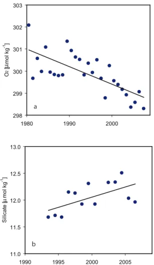
ter, which consequently also resulted in a warming of the Greenland Sea Deep Water (Blindheim and Rey, 2004; Blindheim and Østerhus, 2005). Dissolved oxygen and sil-icate data from the deep water at OWSM is plotted in Fig. 9 and a similar picture with decreasing oxygen and increasing silicate concentrations over the years are also seen
BGD
4, 2929–2958, 2007 Inorganic carbon time series I. Skjelvan et al. Title Page Abstract Introduction Conclusions References Tables Figures ◭ ◮ ◭ ◮ Back CloseFull Screen / Esc
Printer-friendly Version Interactive Discussion
EGU
here. The change has not been as extensive as in the Greenland Sea, though, with the regression lines showing a decrease in oxygen of about 0.08 µmol kg−1yr−1and an increase in silicate of about 0.04 µmol kg−1yr−1. However, the same conclusion can be drawn for the deep Norwegian Sea as for the deep Greenland Sea, that the fraction of the old Arctic Ocean Deep Water has increased compared to previous years. To
deter-5
mine the change in the deep inorganic carbon caused by the changes in water mass composition a Redfield ratio between carbon and oxygen (Rc:o) of 106:–138 is used (Redfield et al., 1963), and the increase of carbon in the deep water due to decay of or-ganic matter is determined to be 0.06 µmol kg−1yr−1. This natural process represents about 10% of the observed carbon increase of 0.57 µmol kg−1yr−1, and consequently,
10
there must be additional explanations for the observed deep water carbon increase at OWSM.
From the eMLR method a deep water anthropogenic CT increase of about 9 µmol kg−1 over 24 years is estimated. This equals an annual increase of about
0.4 µmol kg−1, which represents the major part of the observed deep water
car-15
bon increase at OWSM, and in the following some possible sources for this anthro-pogenic increase will be discussed. Olsen et al. (2006) estimated an anthroanthro-pogenic increase in surface water CT in the Greenland Sea surface water of between 0.6 and
0.7 µmol kg−1yr−1. It is reasonable to assume that with an annual deep convection down to about 1500 m in the Greenland Sea (Ronski and Bud ´eus, 2005) the convected
20
water will spread out along isopycnals and enter the deep water circulation, of which a branch is the cyclonic circulation in the Norwegian Sea. It is also reasonable to assume that this transport route might take about 5 years (assuming a deep current speed of 1 cm s−1, which is a tenth of the speed in Orvik et al. (2001), who observed an average
current speed of the deep water at 64◦N 1.5◦E of about 10 cm s−1). Along the way
25
from the Greenland Sea to OWSM the water is mixed with surrounding waters and the anthropogenic signal might be diluted, but it is difficult to estimate to which extent.
The observed deep water CT increase at OWSM might also be explained by turning
Ice-BGD
4, 2929–2958, 2007 Inorganic carbon time series I. Skjelvan et al. Title Page Abstract Introduction Conclusions References Tables Figures ◭ ◮ ◭ ◮ Back CloseFull Screen / Esc
Printer-friendly Version Interactive Discussion
EGU
landic Sea is transported further east to join the cyclonic circulation in the deep Norwe-gian Sea, and this is based on the observed similar characteristics of bottom waters in the Iceland Sea and the deep Norwegian Sea. According to J ´onsson (1992) the strong and positive wind-stress curl during winter in the centre of the Icelandic gyre might give reason to deep convection in this area, and hereby bringing an anthropogenic carbon
5
signal down in the water column. A fraction of this newly formed Iceland Sea Deep Wa-ter enWa-ters the south-wesWa-tern Norwegian Sea, joins the cyclonic gyre there, and finally reaches the OWSM deep water. Another source is found by addressing the recircu-lated Atlantic Water, which has its origin in the northward flowing Norwegian Atlantic Current where it has got its anthropogenic signal (about 1 µmol kg−1yr−1to the north of
10
the Boreas Basin surface water according to Olsen et al., 2006). It is sub-ducted in the Fram Strait, and a fraction returns southwards into the Nordic Seas as a component of the East Greenland Current (Rudels et al., 1999). A part of this water continues into the Iceland Sea and enters the East Icelandic Current (e.g. Rudels et al., 2002). On its way the recirculated water is modified due to mixing with surrounding waters and part
15
of this water might finally enter the south-western Norwegian Sea and join the cyclonic circulation of the Norwegian Sea Deep Water. The time from the Atlantic Water leaves the surface to it appears in OWSM deep water is less than 10 years based on an ef-fective current speed of 1 cm s−1. In these ways an anthropogenic signal might have been transported towards OWSM via the Iceland Sea and give rise to the observed
20
and estimated annual increase in deep water carbon.
6 Summary
Observations of inorganic carbon, nutrients, and hydrography at OWSM in the Norwe-gian Sea show that over years carbon has increased in the whole water column, and at a higher rate in the surface water compared to the deep water. This increase is verified
25
by an extended multi linear regression method (eMLR). In the surface layer the carbon increase, converted to pCO2, is larger than the observed atmospheric increase, which
BGD
4, 2929–2958, 2007 Inorganic carbon time series I. Skjelvan et al. Title Page Abstract Introduction Conclusions References Tables Figures ◭ ◮ ◭ ◮ Back CloseFull Screen / Esc
Printer-friendly Version Interactive Discussion
EGU
is in contradiction to model results.
The observed deep water carbon increase is of both natural and anthropogenic origin and has several possible explanations; (a) remineralisation due to increased fraction of old Arctic Ocean Deep Water; (b) anthropogenic carbon input via the Greenland Sea surface water; (c) Iceland Sea surface water with a certain anthropogenic carbon
5
signal; and (d) anthropogenic carbon transported with the recirculated Atlantic Water. Remineralisation of organic matter represents about 10% of the deep water carbon in-crease observed at OWSM, but the pathways of the anthropogenic sources are difficult to quantify.
Acknowledgements. Financial support from the Bjerknes Centre for Climate Research (BCCR)
10
and the Geophysical Institute, University of Bergen, is greatly appreciated. The authors are grateful to the captains and crews of M/S Polarfront who kindly did all the water sampling, and to the shipping company Misje Rederi and the Norwegian Meteorological Institute, which gave us permission to use the ship. F. C. Svendsen kindly provided all the bottle salinity data. We also would like to thank our colleagues for fruitful discussions.
15
References
Anderson, L. G. and Olsen, A.: Air-sea flux of anthropogenic carbon dioxide in the North At-lantic, Geophys. Res. Lett., 29, 1835, doi:10.1029/2002GL014820, 2002.
Blindheim, J. and Rey, F.: Water-mass formation and distribution in the Nordic Seas during the 1990s, ICES J. Mar. Sci., 61, 846–863, 2004.
20
Blindheim, J. and Østerhus, S.: The Nordic Seas, Main Oceanographic Features, in: The Nordic Seas – An integrated perspective, AGU Geophysical Monograph, 158, edited by: Drange, H., Dokken, T., Furevik, T., Gerdes, R., and Berger, W., 11–37, 2005.
Dale, T., Rey, F., and Heimdal, B.: Seasonal development of phytoplankton at a high latitude oceanic site, Sarsia, 84, 419–435, 1999.
25
DOE: Handbook of methods for the analysis of the various parameters of the carbon dioxide system in sea water, ver. 2, edited by.: Dickson, A. G. and Goyet, C., ORNL/CDIAC-74, 1994.
BGD
4, 2929–2958, 2007 Inorganic carbon time series I. Skjelvan et al. Title Page Abstract Introduction Conclusions References Tables Figures ◭ ◮ ◭ ◮ Back CloseFull Screen / Esc
Printer-friendly Version Interactive Discussion
EGU
Falck, E. and Anderson, L. G.: The dynamics of the carbon cycle in the surface water of the Norwegian Sea, Mar. Chem., 94, 43–53, 2005.
Friis, K., K ¨ortzinger, A., P ¨atsch, J., and Wallace, D. W. R.: On the temporal increase of anthro-pogenic CO2 in the subpolar North Atlantic, Deep-Sea Res. Pt. I, 52, 681–698, 2005. Gislefoss, J. S., Nydal, R., Slagstad, D., Sonninen, E., and Holm ´en, K.: Carbon time series in 5
the Norwegian Sea, Deep-Sea Res. Pt. I, 45, 433–460, 1998.
Gruber, N., Sarmiento, J. L., and Stocker, T. F.: An improved method for detecting anthro-pogenic CO2in the oceans, Global Biogeochem. Cy., 10, 809–837, 1996.
IPCC, WP1 AR4 Report: The technical summary, in: The Intergovernmental Panel on Climate Change 4th Assessment Report, available at: http://www.ipcc.ch/, 2007.
10
Johnson, K. M., Wills, K. D., Butler, D. B., Johnson, W. K., and Wong, C. S.: Coulometric total carbon dioxide analysis for marine studies, Mar. Chem., 44, 167–187, 1993.
J ´onsson, S.: The sources of fresh water in the Iceland Sea and the mechanisms governing its interannual variability, ICES Marine Science Symposia, 195, 62–67, 1992.
Kara, A. B., Rochford, P. A., and Hurlburt, H. E.: An optimal definition for ocean mixed layer 15
depth, J. Geophys. Res., 105, 16 803–16 821, 2000.
Lewis, E. and Wallace, D. W. R.: Program Developed for CO2 System Calculations, ORNL/CDIAC-105, Carbon Dioxide Information Analysis Center, Oak Ridge National Lab-oratory, U.S. Department of Energy, Oak Ridge, Tennessee, 1998.
Mosby, H.: Water, salt and heat balance of the North Polar Sea and of the Norwegian Sea, 20
Geophysica Norvegica, 24, 289–313, 1962.
Nilsen, J. E. Ø. and Falck, E.: Variations of Mixed Layer Properties in the Norwegian Sea for the period 1948-1999, Prog. Oceanogr., 70, 58–90, 2006.
Olsen, A., Omar, A. M., Bellerby, R. G. J., Johannessen, T., Ninnemann, U., Brown, K. R., Ols-son, K. A., OlafsOls-son, J., Nondal, G., Kivim ¨ae, C., Kringstad, S., Neill, C., and Olafsdottir, S.: 25
Magnitude and Origin of the Anthropogenic CO2Increase and13C Suess Effect in the Nordic Seas Since 1981, Global Biogeochem. Cy., 20, GB3027, doi:10.1029/2005GB002669, 2006.
Omar, A. and Olsen, A.: Reconstructing the time history of the air-sea CO2disequilibrium and its rate of change in eastern subpolar North Atlantic, 1972–1989, Geophys. Res. Lett., 33, 30
L04602, doi:10.1029/2005GL025425, 2006.
Orvik, K. A., Skagseth, Ø., and Mork, M.: Atlantic Inflow to the Nordic Seas: current structure and volume fluxes from moored current meters, VM-ADCP and SeaSOAR-CTD
observa-BGD
4, 2929–2958, 2007 Inorganic carbon time series I. Skjelvan et al. Title Page Abstract Introduction Conclusions References Tables Figures ◭ ◮ ◭ ◮ Back CloseFull Screen / Esc
Printer-friendly Version Interactive Discussion
EGU
tions, 1995–99, Deep-Sea Res. Pt. I, 48, 937–957, 2001.
Redfield, A. C., Ketchum, B. H., and Richards, F. A.: The influence of organisms on the compo-sition of seawater, in: The Sea, edited by: Hill, M. N., John Wiley, New York, 26–77, 1963. Rey, F.: Phytoplankton: The grass of the sea, in: The Norwegian Sea Ecosystem, edited by:
Skjoldal, H. R., Tapir, Trondheim, Norway, 93–132, 2004. 5
Ronski, S. and Bud ´eus, G.: Time series of winter convection in the Greenland Sea, J. Geophys. Res., 110, C04015, doi:10.1029/2004JC002318, 2005.
Rudels, B., Friederich, H. J., and Quadfasel, D.: The Arctic circumpolar boundary current, Deep-Sea Res. Pt. II, 46, 1023–1062, 1999.
Rudels, B., Fahrbach, E., Meincke, J., Bud ´eus, G., and Eriksson, P.: The East Greenland 10
Current and its contribution to the Denmark Strait overflow, ICES J. Mar. Sci., 59, 1133– 1154, 2002.
Sabine, C. L., Key, R. M., Johnson, K. M., Millero, F. J., Poisson, A., Sarmiento, J. L., Wal-lace, D. W. R., and Winn, C. D.: Anthropogenic CO2 inventory of the Indian Ocean, Global Biogeochem. Cy., 13, 179–198, 1999.
15
Schlosser, P., B ¨onisch, G., Rhein, M., and Bayer, R.: Reduction of Deepwater Formation in the Greenland Sea During the 1980s: Evidence from Tracer Data, Science, 251, 1054–1056, 1991.
Skjelvan, I., Olsen, A., Anderson, L. G., Bellerby, R. G. J., Falck, E., Kasajima, Y., Kivim ¨ae, C., Omar, A., Rey, F., Olsson, K. A., Johannessen, T., and Heinze, C.: A Review of the Inorganic 20
Carbon Cycle of the Nordic Seas and Barents Sea, in: The Nordic Seas – An integrated perspective, AGU Geophysical Monograph, 158, edited by: Drange, H., Dokken, T., Furevik, T., Gerdes, R., and Berger, W., 157–175, 2005.
Swift, J. H. and Koltermann, K. P.: The origin of Norwegian Sea deep-waters, J. Geophys. Res., 93, 3563–3569, 1988.
25
Takahashi, T., Sutherland, S. C., Sweeney, C., Poisson, A., Metzl, N., Tilbrook, B., Bates, N., Wanninkhof, R., Feely, R. A., Sabine, C., Olafsson, J., and Nojiri, Y.: Global sea-air CO2 flux based on climatological surface ocean pCO2, and seasonal biological and temperature effects, Deep-Sea Res. Pt. II, 49, 1601–1622, 2002.
Tanhua, T. and Wallace, D. W. R.: Consistency of TTO-NAS inorganic carbon data with modern 30
measurements, Geophys. Res. Lett., 32, L14618, doi:10.1029/2005GL023248, 2005. Tans, P. P. and Conway, T. J.: Monthly Atmospheric CO2Mixing Ratios from the NOAA CMDL
Com-BGD
4, 2929–2958, 2007 Inorganic carbon time series I. Skjelvan et al. Title Page Abstract Introduction Conclusions References Tables Figures ◭ ◮ ◭ ◮ Back CloseFull Screen / Esc
Printer-friendly Version Interactive Discussion
EGU
pendium of Data on Global Change, Carbon Dioxide Information Analysis Center, Oak Ridge National Laboratory, U.S. Department of Energy, Oak Ridge, Tenn., U.S.A, 2005.
Wallace, D. W. R.: Monitoring global ocean carbon inventories, OOSDP Background Report No. 5, Texas A&M University, College Station, Texas, USA, pp. 54, 1995.
Wallace, D. W. R.: Storage and transport of excess CO2 in the oceans: The JGOFS/WOCE 5
global CO2 Survey, in: Ocean circulation and climate: observing and modelling the global ocean, edited by: Siedler, G., Church, J., and Gould, J., 489–521, 2001.
Østerhus, S. and Gammelsrød, T.: The abyss of the Nordic Seas is warming, J. Climate, 2, 3297–3304, 1999.
BGD
4, 2929–2958, 2007 Inorganic carbon time series I. Skjelvan et al. Title Page Abstract Introduction Conclusions References Tables Figures ◭ ◮ ◭ ◮ Back CloseFull Screen / Esc
Printer-friendly Version Interactive Discussion
EGU
Table 1. Typical values of CT, nitrate, silicate, temperature, and salinity at OWSM.
CT Nitrate Silicate Temperature Salinity
[µmol kg−1] [µmol kg−1] [µmol kg−1] [◦C]
Surface winter 2140 11.5 5 7 35.2
Surface summer 2040 ∼ 0 0.5–1 12 34.6–35.1
BGD
4, 2929–2958, 2007 Inorganic carbon time series I. Skjelvan et al. Title Page Abstract Introduction Conclusions References Tables Figures ◭ ◮ ◭ ◮ Back CloseFull Screen / Esc
Printer-friendly Version Interactive Discussion
EGU Table 2. Parameters and coefficients of Eq. (1) for the two different datasets TTO-NAS (1981)
and OWSM (2005) determined from the eMLR approach, and statistics connected to the pre-dicted CT.
Salinity Nitrate Silicate θ
a b c d e σ R2 n
TTO-NAS –1441.67 101.55 3.31 –0.20 –6.65 4.12 0.99 85
OWSM 524.52 45.88 4.66 –2.88 –5.41 5.63 0.95 162
θis the potential temperature.
a, b, c, d , and e are regression coefficients specific for the particular dataset.
σ,R2, and n are the standard deviation, relative predictive power of the model, and number of data points used, respectively.
BGD
4, 2929–2958, 2007 Inorganic carbon time series I. Skjelvan et al. Title Page Abstract Introduction Conclusions References Tables Figures ◭ ◮ ◭ ◮ Back CloseFull Screen / Esc
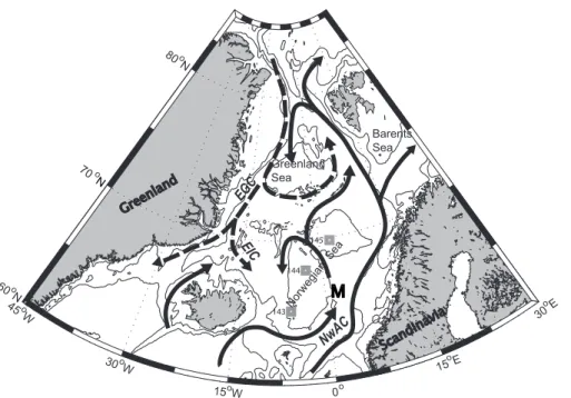
Printer-friendly Version Interactive Discussion EGU 45o W 30o W 15o W 0o 15 oE 30 oE 60o N 70o N 80o N Greenland Sea M EG C Nw AC EIC Barents Sea 143 144 145 Gree nland Scan dinav ia Norw egia n Se a
Fig. 1. Schematic of the northern North Atlantic Ocean. The solid lines indicate the flow
of warm Atlantic Water and the dashed lines show the flow of cold Polar and Arctic Water. NwAC is the Norwegian Atlantic Current, EGC is the East Greenland Current, and EIC is the East Icelandic Current. M denotes Ocean Weather Station M (OWSM) and the grey squares indicate TTO stations used for estimating anthropogenic carbon increase at OWSM.
BGD
4, 2929–2958, 2007 Inorganic carbon time series I. Skjelvan et al. Title Page Abstract Introduction Conclusions References Tables Figures ◭ ◮ ◭ ◮ Back CloseFull Screen / Esc
Printer-friendly Version Interactive Discussion EGU 0 2.5 5 7.5 10 12.5 15 2 2 2 2 4 4 4 4 4 4 6 6 6 6 6 6 8 8 8 8 8 8 8 0 0 0 0 10 10 10 10 10
Ocean Data View
2002 2003 2004 2005 2006 2007 2000 1500 1000 500 0 Depth [m]
BGD
4, 2929–2958, 2007 Inorganic carbon time series I. Skjelvan et al. Title Page Abstract Introduction Conclusions References Tables Figures ◭ ◮ ◭ ◮ Back CloseFull Screen / Esc
Printer-friendly Version Interactive Discussion EGU 0 500 1000 1500 2000 2020 2040 2060 2080 2100 2120 2140 2160 2180 D e p th [ m ] 0 500 1000 1500 2000 0 5 10 15 20 D e p th [ m ] 0 500 1000 1500 2000 0 2 4 6 8 10 12 14 D e p th [ m ] a b c
BGD
4, 2929–2958, 2007 Inorganic carbon time series I. Skjelvan et al. Title Page Abstract Introduction Conclusions References Tables Figures ◭ ◮ ◭ ◮ Back CloseFull Screen / Esc
Printer-friendly Version Interactive Discussion EGU 2020 2060 2100 2140 2180 2001 2002 2003 2004 2005 2006 2007 C T [µ m o l kg -1] 0 4 8 12 16 2001 2002 2003 2004 2005 2006 2007 N it ra te [µ m o l kg -1] 0 4 8 12 2001 2002 2003 2004 2005 2006 2007 S il ica te [ µ m o l k g -1] a b c 34.8 34.9 35.0 35.1 35.2 35.3 35.4 2001 2002 2003 2004 2005 2006 2007 S a li n it y -2 0 2 4 6 8 10 12 14 2001 2002 2003 2004 2005 2006 2007 T e m p e ra tu re [ oC ] d e
Fig. 4. Seasonal variations in (a) CT, (b) nitrate, (c) silicate, (d) temperature, and (e) salinity
at different depths as a function of time. Red squares are at 10 m, green crosses are at 50 m, blue circles are at 200 m, and black filled triangles are at 2000 m depth.
BGD
4, 2929–2958, 2007 Inorganic carbon time series I. Skjelvan et al. Title Page Abstract Introduction Conclusions References Tables Figures ◭ ◮ ◭ ◮ Back CloseFull Screen / Esc
Printer-friendly Version Interactive Discussion EGU 2120 2125 2130 2135 2140 2145 2150 2001 2002 2003 2004 2005 2006 2007 n C T [ µ m o l kg -1] 2120 2125 2130 2135 2140 2145 2150 2001 2002 2003 2004 2005 2006 2007 n C T [ µ m o l kg -1] 2150 2155 2160 2165 2170 2175 2001 2002 2003 2004 2005 2006 2007 n C T [µ m o l kg -1] a b c
Fig. 5. Salinity normalized carbon concentration over the period 2002–2006 in (a) the surface
water during the winter months January to March, (b) the mixed layer during the winter months January to March, and (c) the deep water (four times a year in 2002–2004, and once a month from 2005 and onwards). The surface CT samples are normalized to a salinity of 35.1, while the deep water samples are normalized to a salinity of 34.91.
BGD
4, 2929–2958, 2007 Inorganic carbon time series I. Skjelvan et al. Title Page Abstract Introduction Conclusions References Tables Figures ◭ ◮ ◭ ◮ Back CloseFull Screen / Esc
Printer-friendly Version Interactive Discussion EGU -2 0 2 4 6 8 10 12 14 34.8 34.9 35 35.1 35.2 35.3 35.4 salinity te m p e ra tu re [ oC ] TTO 143 TTO 144 TTO 145 OWSM 2005 a -2 0 2 4 6 8 10 12 14 0 5 10 15 silicate [µmol kg-1] th e ta [ oC ] TTO 143 TTO 144 TTO 145 OWSM 2005 b Deep water Surface water ca 100 m
Fig. 6. (a) Temperature vs. salinity and (b) theta (potential temperature) vs. silicate, based on
data from TTO-NAS stations 1981 (different blue symbols, see Fig. 1) and OWSM 2005 (red crosses).
BGD
4, 2929–2958, 2007 Inorganic carbon time series I. Skjelvan et al. Title Page Abstract Introduction Conclusions References Tables Figures ◭ ◮ ◭ ◮ Back CloseFull Screen / Esc
Printer-friendly Version Interactive Discussion EGU 0 500 1000 1500 2000 -30 -20 -10 0 10 20 30 residual CT [µmol kg -1 ] D e p th [ m ]
Fig. 7. Residuals of CT (measured minus predicted value) as a function of depth; TTO-NAS
1981 (squares) and at OWSM 2005 (crosses). The shaded area indicates the accuracy of the eMLR method of ±7 µmol kg−1
BGD
4, 2929–2958, 2007 Inorganic carbon time series I. Skjelvan et al. Title Page Abstract Introduction Conclusions References Tables Figures ◭ ◮ ◭ ◮ Back CloseFull Screen / Esc
Printer-friendly Version Interactive Discussion EGU 0 500 1000 1500 2000 0 5 10 15 20 25 30 35 40 ∆CT ant [µmol kg-1] D e p th [ m ]
Fig. 8. Amount of anthropogenic carbon entered into the water column at OWSM from 1981
to 2005. The shaded area indicates that in the upper waters the method is less accurate than deeper in the water column.
BGD
4, 2929–2958, 2007 Inorganic carbon time series I. Skjelvan et al. Title Page Abstract Introduction Conclusions References Tables Figures ◭ ◮ ◭ ◮ Back CloseFull Screen / Esc
Printer-friendly Version Interactive Discussion EGU 298 299 300 301 302 303 1980 1990 2000 O 2 [ µ m o l kg -1 ] a 11.0 11.5 12.0 12.5 13.0 1990 1995 2000 2005 S il ica te [ µ m o l kg -1 ] b
Fig. 9. Annual means of (a) dissolved oxygen and (b) silicate over the years at 2000 m depth