Seasonal cycles and variability of O₃ and H₂O in the UT/LMS during SPURT

HAL Id: hal-00301715

https://hal.archives-ouvertes.fr/hal-00301715

HAL is a multi-disciplinary open access

archive for the deposit and dissemination of sci-entific research documents, whether they are pub-lished or not. The documents may come from teaching and research institutions in France or abroad, or from public or private research centers.

L’archive ouverte pluridisciplinaire HAL, est destinée au dépôt et à la diffusion de documents scientifiques de niveau recherche, publiés ou non, émanant des établissements d’enseignement et de recherche français ou étrangers, des laboratoires publics ou privés.

Seasonal cycles and variability of O3 and H2O in the

UT/LMS during SPURT

M. Krebsbach, C. Schiller, D. Brunner, G. Günther, M. I. Hegglin, D.

Mottaghy, M. Riese, N. Spelten, H. Wernli

To cite this version:

M. Krebsbach, C. Schiller, D. Brunner, G. Günther, M. I. Hegglin, et al.. Seasonal cycles and variabil-ity of O3 and H2O in the UT/LMS during SPURT. Atmospheric Chemistry and Physics Discussions, European Geosciences Union, 2005, 5 (4), pp.7247-7282. �hal-00301715�

ACPD

Print Version Interactive Discussion

EGU

Atmos. Chem. Phys. Discuss., 5, 7247–7282, 2005 www.atmos-chem-phys.org/acpd/5/7247/

SRef-ID: 1680-7375/acpd/2005-5-7247 European Geosciences Union

Atmospheric Chemistry and Physics Discussions

Seasonal cycles and variability of O

₃

and

H

₂

O in the UT/LMS during SPURT

M. Krebsbach1, C. Schiller1, D. Brunner2, G. G ¨unther1, M. I. Hegglin2, D. Mottaghy3, M. Riese1, N. Spelten1, and H. Wernli4

1

Institute for Chemistry and Dynamics of the Geosphere: Stratosphere, Research Centre J ¨ulich GmbH, J ¨ulich, Germany

2

Institute for Atmospheric and Climate Science, Federal Institute of Technology, Zurich, Switzerland

3

Applied Geophysics, RWTH Aachen University, Aachen, Germany

4

Institute for Atmospheric Physics, University of Mainz, Mainz, Germany

Received: 13 July 2005 – Accepted: 11 August 2005 – Published: 22 August 2005 Correspondence to: M. Krebsbach ([email protected])

ACPD

Print Version Interactive Discussion

EGU

Abstract

Airborne high resolution in situ measurements of a large set of trace gases including ozone (O₃) and total water (H₂O) in the upper troposphere and the lowermost strato-sphere (UT/LMS) have been performed above Europe within the SPURT project. With its innovative campaign concept, SPURT provides an extensive data coverage of the

5

UT/LMS in each season within the time period between November 2001 and July 2003. Ozone volume mixing ratios in the LMS show a distinct spring maximum and autumn minimum, whereas the O₃ seasonal cycle in the UT is shifted by 2 to 3 month later towards the end of the year. The more variable H₂O measurements reveal a maxi-mum during spring/summer and a minimaxi-mum during autumn/winter with no phase shift

10

between the two atmospheric compartments.

For a comprehensive insight into trace gas composition and variability in the UT/LMS several statistical methods are applied using chemical, thermal and dynamical vertical coordinates. In particular, 2-dimensional probability distribution functions serve as a tool to transform localised aircraft data to a more comprehensive view of the probed

15

atmospheric region. It appears that both trace gases, O₃ and H₂O, reveal the most compact arrangement and are best correlated in the view of potential vorticity (PV) and distance to the local tropopause, indicating an advanced mixing state on these surfaces. Thus, strong gradients of PV seem to act as a transport barrier both in the vertical and the horizontal direction. The alignment of trace gas isopleths reflects

20

the existence of a year-round extra-tropical tropopause transition layer. The SPURT measurements reveal that this layer is mainly affected by stratospheric air during win-ter/spring and by tropospheric air during autumn/summer.

Mixing entropy values for O₃and H₂O in the LMS appear to be maximal during spring and summer, respectively, indicating highest variability of these trace gases during the

25

ACPD

Print Version Interactive Discussion

EGU

1. Introduction

Ozone and water vapour are important absorbers of solar irradiance and emit-ters/absorbers of terrestrial radiation. Both species have direct and indirect effects on radiative forcing and/or photolysis rates and play therefore a decisive role for the radiative budget of several atmospheric regions, for chemistry and climate. They are

5

further suitable trace gases to investigate and understand transport and mixing pro-cesses, especially in the region of the upper troposphere and lowermost stratosphere (UT/LMS). This part of the atmosphere is to a large extent affected by dynamics, and in particular by bi-directional stratosphere-troposphere exchange. Trace gas distributions in the UT/LMS depend strongly on the interaction between dynamical and chemical

10

processes near the tropopause. Changes in the chemical composition of the UT/LMS have strong impact on atmospheric radiation. A detailed understanding of the trace gas distributions, their variability, underlying processes and transport mechanisms of natu-ral and anthropogenic emissions is crucial for climate prediction and radiative feedback mechanisms, in particular, when considering global warming scenarios (e.g.Lindzen,

15

1990;Rind et al., 1991;Inamdar and Ramanathan,1998) and in climate simulations

(e.g.McLinden et al.,2000). The UT/LMS and especially the tropopause region is thus of significant scientific interest.

Several data sets of satellite instruments have been analysed to infer seasonal dis-tributions of ozone and water vapour in the LMS as well as connected transport

mech-20

anisms. From SAGE II measurements, Pan et al. (1997) inferred ozone and water vapour distributions in the LMS and compared them to MLS and ER-2 measurements

(Pan et al., 2000). MLS water vapour data was further investigated by Stone et al.

(2000) regarding climatological aspects as well as spatial and temporal variability.

Ran-del et al. (2001) andPark et al.(2004) used HALOE data to derive seasonal variation

25

of water vapour in the LMS. Furthermore, ozone and water vapour data in the UT and LMS from POAM III measurements were analysed by Prados et al. (2003) and

ACPD

Print Version Interactive Discussion

EGU

for a global data coverage of the whole atmosphere. However, there are several dis-advantages and restrictions given by nature and technology, in particular, the limited spatial resolution. Due to the restrictions and the lack of satellite data in the UT/LMS, the tropopause region is rather under-sampled. Highly accurate and resolved obser-vations of the UT/LMS can only be achieved with in situ measurements. For instance,

5

Strahan(1999) analysed ozone data from ER-2 flights in the potential temperature

re-gion between 360 K and 530 K. Anyhow, aircraft measurements are commonly quite sporadically distributed in time and space. For such purposes, projects like MOZAIC (e.g.Marenco et al.,1998), NOXAR (e.g.Brunner et al.,1998) or CARIBIC (e.g.

Bren-nikmeijer et al., 2005) use commercial and passenger aircraft to measure routinely

10

chemical species. However, thereby only the lower part of the LMS is reached.

A cutting edge for a new concept of aircraft campaigns was introduced by the very successful project SPURT (German: SPURenstofftransport in der Tropopausenregion, trace gas transport in the tropopause region). Within the European sector (30◦ E to 30◦ W, 30◦ N to 80◦ N) an extensive and continuous high quality data coverage of

15

the UT and LMS in each season was obtained. Using a Learjet 35A a total of eight campaigns, evenly distributed in time between November 2001 and July 2003, were performed. Depending on meteorological conditions, the aircraft’s ceiling altitude is about 14 km and thus allows for sampling in the LMS during all seasons, even at sub-tropical latitudes. The SPURT measurements between the 280 K and 380 K isentropes

20

thus contribute significantly to the data coverage in the whole extra-tropical LMS above Europe. A description of the project strategy, its aims, performance and instrumentation is given in an overview paper byEngel et al.(2005).

The purpose of this work is to analyse the seasonality and variability of ozone (O₃) and total water (H₂O) in the UT/LMS as measured during the SPURT project. After

25

a short description of these trace gas measurements, the seasonal cycles of O₃ and H₂O are discussed. Several statistical perspectives are used to investigate trace gas variability and implications for the trace gas distribution in the probed atmospheric re-gion.

ACPD

Print Version Interactive Discussion

EGU

2. The SPURT O₃and H₂O data

During the SPURT campaigns, O₃ was measured with UV absorption by the JOE in-strument (J ¨ulich Ozone Experiment) (Mottaghy,2001). For most flights, i.e. from the third campaign on, O₃ was additionally measured by a chemiluminescence detector ECO-Physics CLD 790-SR (Hegglin,2004). Intercomparison of both instruments

re-5

sults in high consistency (Hegglin,2004;Engel et al.,2005). However, in the presented analyses here the JOE data is preferably considered and ECO data are only used if no JOE data are available. Total water, i.e. the sum of vapour and vaporised ice, was mea-sured with the photofragment-fluorescence technique by the FISH instrument (Fast In situ Stratospheric Hygrometer) (Z ¨oger et al.,1999). The instruments JOE, ECO and

10

FISH have a time resolution of 10, 1, 1 s, and an accuracy of 5, 5, 6%, respectively. Due to the different integration times of the single instruments the measurement data was analysed as 5 s data. Thereby, the JOE data was interpolated to the centre inter-val, measurements with a higher sampling rate were averaged over each 5 s. For an average aircraft flight speed of 150 to 200 m s−1this results in a mean spatial resolution

15

of 0.75 to 1.00 km. For a complete listing of the Learjet payload, data availability, and for details about the processing of the whole SPURT data set seeEngel et al.(2005).

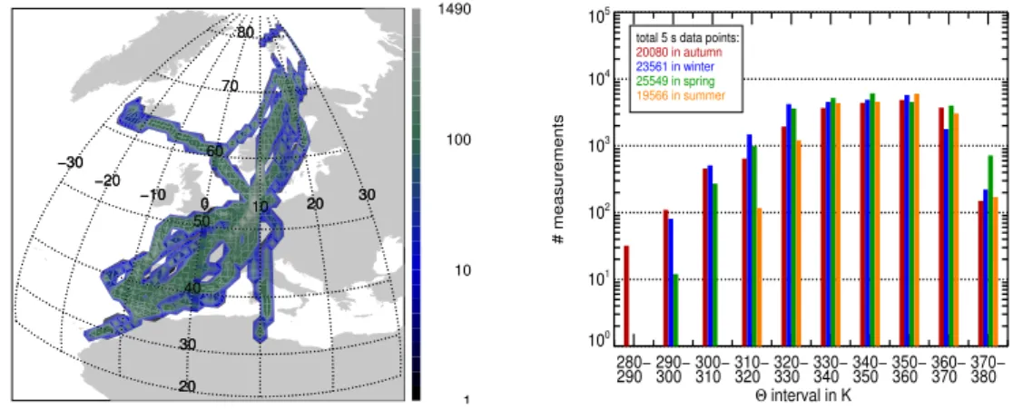
Figure1 gives an impression of the obtained coverage of O₃ and/or H₂O measure-ments during SPURT in the geographical and potential temperature space. The map in the left panel reflects the number of measurements in a 1◦ longitude × 1◦ latitude

20

bin. Each campaign consisted of a minimum of 2 flight days. On one day southbound and on the other day northbound flights were performed from and back to the Learjet basis Hohn (9.53◦ E, 54.31◦ N, northern Germany). The contours clearly accentuate the basis in northern Germany as well as the two main inter-stations, Faro in southern Portugal for the southbound flights and Tromsø in Norway for the northbound flights.

25

Slow ascents and descents in these regions result in a large number of measurements there. Each season (autumn, winter, spring, and summer, corresponding to the months SON, DJF, MAM, and JJA) was investigated with two campaigns.

ACPD

Print Version Interactive Discussion

EGU

The right panel of Fig. 1 shows frequency distributions of data points in potential temperature intervals from 280 K to 380 K in steps of 10 K. Potential temperature (Θ) is calculated from avionic measurements of pressure (p) and temperature (T ). It indi-cates winter and spring with more than 23 000 and 25 000 data points, respectively, as the best captured seasons for O₃ and H₂O. With more than 19 000 data points also

5

the autumn and summer season are probed quite well. The tail at the lowerΘ values between 280 K and 310 K is a result of sampling, since the inlet of the FISH instrument was only opened at altitudes higher than a pressure value of ≈400 hPa. Similarly, the JOE instrument provides high qualitative data rather at altitudes above that pressure level. The frequency distributions in the Θ space reflects the SPURT concept of the

10

flight profiles. Slow ascents and descents allowed for accurately resolved slant vertical profiles. Within each mission two flight legs at rather constant pressure altitude were performed, one near and the other above the tropopause (cf. numbers of data points within 320 K and 340 K and 350 K and 370 K, respectively). Due to fuel consumption and thus lower mass of the aircraft, at the end of each mission a climb to maximum

15

altitude (>370 K) was performed to sample generally undisturbed stratospheric back-ground air. The altitude flight profile was mirrored on the mission back to Hohn to sample the meteorological condition in two different height regimes.

To place the measurements in a meteorological context, ECMWF (European Centre for Medium-Range Weather Forecasts) analyses with a time resolution of 6 h and a grid

20

resolution of 1◦×1◦ in longitude and latitude on 21 pressure levels between 1000 and 1 hPa are used. Each analysis data set was interpolated to 25 isentropic surfaces lo-cated between 280 K and 400 K in steps of 5 K. On these isentropes potential vorticity (PV) is obtained by spatial and temporal interpolation to the flight tracks. The diagno-sis of PV from meteorological data fields is affected by errors (e.g. Beekmann et al.,

25

1994;Good and Pyle,2004). The procedure of data assimilation will remove obvious

observational errors (Hollingsworth and L ¨onneberg,1989). Anyhow, the accuracy in calculating PV is sensitive to the horizontal and vertical resolution and, in particular, small-scale meteorological features like tropopause folds are hardly represented in

de-ACPD

Print Version Interactive Discussion

EGU

tail in the meteorological analyses. In contrast, in situ measurements have a much finer resolution and can therefore resolve small-scale features. This has to be considered when correlating model derived quantities with in situ measurements (cf. Sect.4).

3. Seasonal cycles of O₃and H₂O in the UT and LMS

In order to derive seasonal cycles of O₃ and H₂O in the UT and LMS, PV is used to

5

categorise air parcels. Since PV increases with height and latitude in the northern hemisphere, it is used here to split the data set into atmospheric subsets. Detailed analyses of vertical profiles during ascents and descents reveal a PV value of 2.0 to 2.5 PVU (1 PVU=10−6m2s−1K kg−1, according toHoskins et al.,1985) as represen-tative for the location of the extra-tropical tropopause during SPURT (e.g.Hoor et al.,

10

2004;Krebsbach,2005; Hegglin et al., in preparation1). Potential vorticity values lower

than 1 PVU are therefore assumed to denote air of the (upper) troposphere, values within the range 1–3 PVU air of the tropopause region, and higher values reflect an increasing stratospheric character of the probed air.

3.1. O₃in the UT and LMS

15

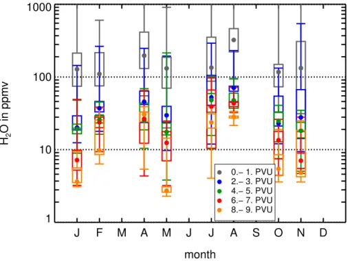
In Fig. 2 monthly median O₃ volume mixing ratios (VMRs) in different PV domains, characteristic for specific regions of the atmosphere, are shown as measured during SPURT. Thereby, a box plot graphing is used, showing centring (median), spread (25 and 75 quartiles), and distribution (minimum and maximum). Thus, an accurate im-pression of the central tendency and variability of O₃ is possible. Considering the

20

complete data set, the seasonal cycle of O₃ in the (upper) troposphere shows a min-imum during winter and a broad spring to summer maxmin-imum. There exists a number

1

Hegglin, M. I., Brunner, D., Peter, Th., Hoor, P., Fischer, H., Staehelin, J., Krebsbach, M., Schiller, C., Parchatka, U., and Weers, U.: Measurements of NO, NO_y, N₂O, and O₃ during SPURT: Seasonal distributions and correlations in the lowermost stratosphere.

ACPD

Print Version Interactive Discussion

EGU

of regions showing a broad summer maximum in tropospheric ozone. The existence of such a maximum is often associated with photochemical production (e.g. Logan,

1985). Thereby, O₃ is formed by reactions involving volatile organic compounds and nitrogen oxide (NO_x), driven by solar radiation. Many of these regions are continental and influenced by pollution (e.g.Logan, 1989; Scheel et al., 1997). Also in the free

5

troposphere, a broad spring to summer maximum was observed (e.g. Logan, 1985;

Schmitt and Volz-Thomas, 1997). Beekmann et al. (1994) showed based on ozone

sonde data from Observatoire de Haute-Provence (OHP) that the seasonal variation of tropospheric O₃ is characterised by a large maximum during spring and summer. Furthermore, LIDAR and ozone sonde measurements from OHP from 1976 to 1995

10

give evidence for a shift from a spring maximum to a spring/summer maximum in the free troposphere (Ancellet and Beekmann,1997). The observed broad spring/summer O₃maximum during SPURT in the UT with a slight shift towards spring is furthermore in accordance with results fromBrunner et al.(2001).

Most variable O₃ VMRs are present during spring. During this season the influence

15

of the large-scale downward motion is most prominent (Appenzeller et al.,1996). Also the net O₃ flux across the extra-tropical tropopause has a peak during spring to early summer, primarily affected by the outward O3 flux of the LMS through the tropopause

(Logan,1999). Thus, the already enhanced tropospheric O₃VMRs during spring seem

to be effected by the downward transport of O3-rich stratospheric air during that

sea-20

son.

Measurements at Mace Head, Ireland, illustrate a clear spring O₃ maximum (

Der-went et al.,1998). However, the appearance of a spring maximum in the O₃seasonal cycle in the northern hemisphere troposphere is heavily debated (cf. review byMonks,

2000). Regarding northbound and southbound flights during SPURT separately (not

25

shown here), the maximum in tropospheric O₃VMRs for higher latitudes occurs during late spring and is shifted to late summer further south (cf. Krebsbach,2005). This is in agreement with results ofScheel et al. (1997) from low-altitude and mountain sites between 28–79◦ N. Further, Hough (1991) showed by 2-dimensional model studies

ACPD

Print Version Interactive Discussion

EGU

the general maximum of O₃ precursors like NO_x, carbon monoxide, and hydrocar-bons in the free troposphere at middle and higher latitudes during winter and spring, which is in accordance with the slight shift towards spring observed during the north-ern SPURT flights. As mentioned before, additionally a contribution to higher O₃VMRs in the UT during spring is presumably affected by a contribution of O3-rich air due

5

to stratosphere-to-troposphere transport. The observed maximum in O₃ VMRs dur-ing summer is possibly a result of in situ photochemical production (e.g.Logan,1985;

Haynes and Shepherd,2000) since photochemical activity is expected to be highest

during this period (e.g.Liu et al.,1987).

For higher PV values, in the LMS, a clear spring maximum and autumn minimum

10

is evident with a peak-to-peak amplitude of ≈400 ppbv O₃ within the PV range of 8–9 PVU. The ozone build-up in this atmospheric region occurs during winter as a consequence of poleward and downward transport, since the lifetime of O₃ is long with respect to chemical loss (e.g. Holton et al., 1995) and is largely controlled by dynamics (Logan,1999). The observed spring maximum in the LMS over Europe

dur-15

ing SPURT is most probably due to the downward advection of high O₃ VMRs by the stratospheric winter/spring Brewer-Dobson circulation, in accordance with e.g.Logan

(1985), Austin and Follows (1991), Oltmans and Levy II (1994), Haynes and

Shep-herd (2000), Prados et al. (2003). Ozone VMRs fall off from March to October with a maximum decrease rate within May to August. Much of this decrease is

presum-20

ably caused by the change in tropopause height and transport mechanisms. On the basis of observations of SAGE II,Pan et al. (1997) andWang et al. (1998) assumed that isentropic cross-tropopause inflow of tropospheric air into the LMS influences the seasonal cycle of O₃ (and H₂O, see Sect. 3.2) in that atmospheric region, especially during summer. A maximum of quasi-isentropic inflow into the LMS during summer

25

was also identified in model studies byChen(1995, 2-dimensional) andEluszkiewicz

(1996, 3-dimensional). Enhanced content of tropospheric air in September compared to May was identified byRay et al.(1999) from balloon-borne chlorofluorocarbons and water vapour measurements, which was also thought to be owing to quasi-isentropic

ACPD

Print Version Interactive Discussion

EGU

in-mixing of tropospheric air. The seasonal cycle of O₃ in the extra-tropics therefore differs between the UT and the LMS. The transition region between the troposphere and the stratosphere (1–3 PVU) is rather influenced by the troposphere. However, just above the tropopause layer (4–5 PVU) the stratospheric signal becomes dominant.

Amplitudes of O₃ VMRs grow with increasing PV. Regarding the progression of O₃

5

VMRs through surfaces of increasing PV, the most prominent increase is apparent during winter and spring, whereas during summer and autumn the gradients are com-parably weak. Since in Fig.2rather dynamically similar air parcels are considered and PV exhibits a transport barrier (cf. e.g. Krebsbach et al., a, in preparation2, and Hegglin et al.), the lower O₃gradients with respect to PV surfaces during summer and autumn

10

suggest an intensified transport of tropospheric air into the LMS during these seasons (cf. Sect. 3.2). Towards higher PV ranges (> 3 PVU), i.e. deeper in the LMS, tropo-spheric influence decreases which results in an increase in the slope (dO₃/dPV). The observed seasonal variation of the slope has a maximum of about 60–90 ppbv/PVU in April and a minimum of 10–30 ppbv/PVU in October. The results are comparable with

15

findings fromBeekmann et al.(1994) andZahn et al.(2004). 3.2. H₂O in the UT and LMS

As ozone, water vapour shows a distinct gradient at the extra-tropical tropopause. Due to the temperature lapse rate and the decrease in pressure, water vapour VMRs de-crease exponentially with height from the troposphere up to the tropopause region.

20

Calculated averages of measurements that span the transition region between the UT and the LMS are dominated by moist air from below the tropopause.

In Fig.3monthly medians of H₂O measured during SPURT are depicted in the same manner as for O₃(cf. Fig.2). Based upon the annual cycle of tropopause temperatures

2

Krebsbach, M., Schiller, C., Spelten, N., G ¨unther, G.: Characteristics of the extra-tropical transition layer as derived from O₃ and H₂O measurements in the UT/LMS during SPURT: I. trace gas distributions and stratosphere-troposphere exchange, a.

ACPD

Print Version Interactive Discussion

EGU

(e.g.Hoinka, 1999) and resulting ice saturation VMRs, maximum H₂O VMRs in the tropopause region are expected during the summer, lowest during the winter months. The SPURT measurements show maximum H₂O VMRs in the (upper) troposphere (0–1 PVU) during the August 2002 campaign. However, the spring campaign in April 2003 shows a secondary maximum, whereas in May 2003 comparably low H₂O VMRs

5

are apparent. This feature pervades through the whole considered PV categories and reflects the high variability of H₂O in the probed atmospheric region. Anyhow, the ten-dency of higher VMRs during summer and lower ones during winter and also autumn is present. Across the tropopause the strong gradient in H₂O is evident. When consid-ering northbound and southbound flights separately, the southern tropopause region

10

is slightly dryer. This is probably due to the higher influence of the dryer sub-tropical regions (see for instanceHoinka,1999;Krebsbach,2005).

In the LMS (>4 PVU) a clearer seasonal cycle in H₂O is apparent with a distinct maximum during summer and a minimum during autumn and winter. This is in agree-ment with previous in situ and remote observations (e.g.Mastenbrook and Oltmans,

15

1983;Foot,1984;Oltmans and Hofmann,1995;Dessler et al.,1995;Pan et al.,1997;

Stone et al.,2000). In contrast to O₃, with increasing PV the H₂O VMRs as well as the

amplitude of the annual cycle decreases (note the logarithmic ordinate). This indicates a more pronounced seasonal cycle of H₂O in the lower LMS.

Air in the so called “overworld” (Hoskins, 1991) is dehydrated as it is transported

20

through the tropical cold trap. However, for a large extent of the performed SPURT campaigns H₂O VMRs are considerably enhanced compared to stratospheric back-ground values of about 2–7 ppmv (e.g.Hintsa et al.,1994). Even in the upper consid-ered PV ranges median H₂O VMRs during summer are about 30 ppmv. These VMRs are much higher than could solely be explained by entry of air into the stratosphere in

25

the tropics (e.g.Foot,1984;Nedoluha et al.,2002). Thus, values substantially greater than 7 ppmv are evidence for transport mechanisms of air into the LMS across the extra-tropical tropopause, and this signature is carried deep into the lower stratospheric region.

ACPD

Print Version Interactive Discussion

EGU

The variability of H₂O for observations in the tropopause region and in the strato-sphere increases from autumn/winter towards summer (see also Sect.4and frequency distributions inKrebsbach,2005). This suggests that the potential for transport of wa-ter through the tropopause is more effective and thus more important and significant during summer. This is especially relevant for long-term transport which is the

com-5

bined effect of mass transport and the efficiency of freeze-drying. Hence, as already derived from the O₃ data, the LMS seems to be more influenced by the troposphere during summer than during winter which is in agreement with the discussed seasonal variability of water vapour in the LMS by e.g.Pan et al.(2000).

Whereas the O₃ maximum in the UT is approximately in phase with the H₂O

maxi-10

mum, it occurs about 2–3 months later (earlier) in the year as the O₃ maximum (mini-mum) in the LMS. A similar time lag was found byPan et al.(1997) andPrados et al.

(2003). Due to the large debate, especially concerning the often observed spring O₃ maximum at some northern hemisphere stations, it is further to investigate to what extent the correlation and/or anti-correlation of both trace gases could be attributed to

15

dynamics or to chemistry. Anyhow, the seasonal cycles of O₃ and H₂O obtained dur-ing the SPURT campaigns underline the influence of two competdur-ing processes in the UT/LMS region: (i) subsidence of dry air from the overworld, which is primarily deter-mined by the low tropical tropopause temperatures and transported by the large-scale Brewer-Dobson circulation (e.g.Holton et al.,1995), and (ii) direct transport of moist air

20

of tropical, sub-tropical or mid-latitude origin across the extra-tropical tropopause (e.g.

Dessler et al.,1995;Hintsa et al., 1998). As is apparent in Fig. 3, in contrast to the

O₃ VMRs, the seasonal cycles of H₂O in the UT and LMS are roughly in phase with each other. This same seasonal course in both atmospheric compartments is a priori not clear. Whereas much of the air in the LMS has probably been transported into the

25

stratosphere by the former process (i), it is likely that local vertical transport processes play a much larger role in determining H₂O in the UT and the lower LMS.

ACPD

Print Version Interactive Discussion

EGU

4. O₃and H₂O in a view from different coordinates

The SPURT measurements covered a broad latitude range with different meteorolog-ical situations, often associated with small-scale phenomena (e.g. tropopause folds) and large-scale meridional advection of polar and/or sub-tropical and/or tropical air. The different dynamical impacts result in discontinuities and changes in the tropopause

5

height, particularly in the vicinity of regions with high wind velocities, the jet streams, in the literature often referred to as the region of the “tropopause break”. In order to get a comprehensive insight into distribution, spreading, ranging, and variability of the mea-sured trace gases in the SPURT region, 2-dimensional probability distribution functions (PDFs) are determined by using chemical, thermal, and dynamical vertical coordinates.

10

Moreover, it is interesting to investigate which coordinate is best correlated with a trace gas and where the most compact correlation appears. An accurate correlation helps to deduce and to assess transport processes and provides the possibility for transforma-tion into related quantities (see e.g. Krebsbach et al., b, in preparatransforma-tion3).

4.1. Probability distribution functions

15

In several SPURT flights, distinct cross-tropopause exchange events and characteristic features for specific meteorological situations could be identified (e.g.Hegglin et al.,

2004, Krebsbach et al., c, in preparation4). To obtain a compact view of the probed atmospheric region, PDFs are a tool to centralise the large number of measurements. As an advantage of the PDFs, all measurement data is considered, and averaging

20

is minimised. Thus, outliers become more visible and the prominent structures and features are revealed (Ray et al.,2004).

3

Krebsbach, M., Schiller, C., Spelten, N., G ¨unther, G.: Characteristics of the extra-tropical transition layer as derived from O₃ and H₂O measurements in the UT/LMS during SPURT: II. extent and seasonal variation, b.

4

Krebsbach, M., Schiller, C., G ¨unther, G., Wernli, H.: Transport across the extra-tropical tropopause and impact on the H₂O content of the LMS, c.

ACPD

Print Version Interactive Discussion

EGU

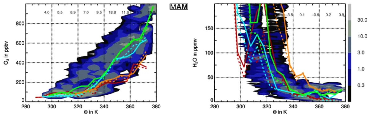
In Fig.4, PDFs of O₃ (left) and H₂O (right) as a function of the thermal vertical co-ordinate potential temperature for the spring season are depicted. For the distributions obtained for the other seasons it is referred toKrebsbach (2005). Ozone is binned by 20 ppbv, H₂O by 2 ppmv, and potential temperature by 5 K. The trace gas distribu-tions are normalised to every bin of the thermal coordinate. This means, the colour

5

coding reflects the probability in percent to measure a certain trace gas VMR at a cer-tain potential temperature. Additionally, the mean and median value in eachΘ bin is represented by the solid and dashed coloured line, respectively. While the mean is an appropriate measure of the central tendency for roughly symmetric distributions, it is misleading when applied to skewed distributions since it can greatly be influenced

10

by extremes. In contrast, the median is less sensitive to outliers and may be more informative and representative for skewed distributions. All seasonal means and medi-ans are displayed to compare to each other (red, blue, green, and orange for autumn, winter, spring, and summer, respectively).

High probabilities, reflected by the light grey/green shadings, are very scattered

15

throughout the O₃ distribution and, although both parameters,Θ and O3, can be con-sidered as a vertical coordinate, no clear correlation is apparent. There is no symmetry around the mean or median values and multiple modes can be noted. Generally, an increase of O₃ VMRs with increasingΘ (height) is present, but the spreading of O3 VMRs on levels with constant potential temperature, the isentropes, is considerably

20

large, resulting in a funnel or wedge structure. However, the large scatter and spread in the O₃distributions is expected, since the O₃VMRs are largely dependent upon the location of the tropopause. The single flight missions extended over a large latitude range. Therefore, the variability of potential temperature at the tropopause location during each deployment along the flight path was sometimes quite large. For instance,

25

on a flight from Hohn to Tromsø on 17 May 2002, the tropopause was located at 304 K in the vicinity of Tromsø and at 328 K near the campaign base Hohn, which is a vari-ation of 24 K (seeKrebsbach,2005). However, also at higher isentropes, i.e. further away from the local tropopause, the spread in O₃VMRs is very high.

ACPD

Print Version Interactive Discussion

EGU

The H₂O PDF shown here as well as the distributions for the other seasons (see

Krebsbach,2005) exhibit similar characteristics as those for O₃. The large variation

of the tropopause location is transparent in the high amounts of H₂O VMRs below ≈340 K, where also in the course of means, and partly of the medians, at lower isen-tropes a strong kink is present. A more compact distribution is only apparent above

5

≈350 K, with the higher variability during the summer season. When shifting the mean H₂O VMRs for the summer PDF by ≈20 K towards lower isentropes, the shape of the mean line (orange) is quite similar to the mean line for the winter season (blue). The SPURT measurements are mainly concentrated in the atmospheric region above isen-tropes of ≈320 K. Thus, a strongest tropospheric influence during summer, as already

10

mentioned in the previous section, is in agreement with the seasonally integrated mass flux through troposphere-to-stratosphere transport bySprenger and Wernli(2003, their Fig. 3b).

The shapes of the trace gas PDFs for the winter and spring measurements are quite different from the distributions obtained for summer and autumn (seeKrebsbach,

15

2005). Whereas the former show a rather steep distribution with rising O₃VMRs and increasing Θ, the latter are more flat or show a prominent wedge structure towards higher isentropes. The large variability of trace gas VMRs, especially at higher isen-tropes (e.g. >400 ppbv O₃ at 360 K during all seasons) and the occurrence of several high probabilities on single isentropes, indicate that quasi-isentropic mixing is rather

20

weak in this region.

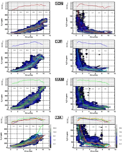
The picture drawn on the basis ofΘ changes significantly when shifting the thermal coordinate to a dynamic coordinate, namely PV. The corresponding trace gas PDFs are shown for all seasons in Fig. 5 with PV incremented in 0.5 PVU steps. As is di-rectly evident, O₃ is much stronger correlated with PV than withΘ, which is rather an

25

accurate height or correlation parameter in the undisturbed stratosphere. The rang-ing of O₃VMRs on surfaces of PV is considerably suppressed when compared to the spreading on isentropes. Even the wedge structure in the autumn and summer distri-butions as a function ofΘ is significantly reduced. The highest probabilities are mostly

ACPD

Print Version Interactive Discussion

EGU

centred in the distributions and symmetrically arranged around the mean or median O₃ VMRs in every PV bin. In the PV-PDFs, additionally the trace gas gradients in depen-dence of the coordinate are calculated within 2 PVU intervals. The O₃/PV-gradients are ≈2–4 times stronger in the 2–4 PVU range than within the interval 0–2 PVU. The means and medians show a slight kink in this range, indicating 2 PVU as a good proxy

5

for the dynamically defined extra-tropical tropopause during the SPURT missions. Of course, the gradient is weaker during summer which is due to the annual cycle of O₃ in the UT and in the LMS. Thus, the distinct seasonal cycles of O₃in both atmospheric compartments, UT and LMS, are clearly apparent.

For H₂O, the spreading in the PDFs is also reduced with PV as the reference

coor-10

dinate. The kink due to the varying location of the local tropopause in theΘ space is not present in the PV space. Also above 2–3 PVU, i.e. within the tropopause region, the variation of H₂O VMRs on PV surfaces is significantly reduced. However, during summer the H₂O distribution is more compact when related toΘ.

As shown by the mean and medians, moreover the seasonal cycles of H₂O in the

15

UT and LMS are reflected in the PDFs, with certainly higher VMRs during the summer months in the UT as well as in the LMS. The trace gas VMRs show a more compact distribution in a dynamical sense. In contrast to the spreading and distribution of sev-eral high probabilities on isentropic surfaces, Fig. 5 reveals that trace gas VMRs are more uniformly distributed and the probabilities vary less on PV surfaces. This

indi-20

cates a more pronounced mixing state of trace gases on these surfaces rather than on isentropic surfaces.

A further coordinate system to look at the trace gas distribution and their variability is a coordinate system centred at the tropopause. Unfortunately, there was no instru-ment aboard the Learjet 35A measuring temperature profiles continuously along the

25

flight track from which the tropopause altitude could be determined after the WMO definition (WMO,1986). Anyhow, the extra-tropical tropopause during SPURT can be derived dynamically from a PV threshold value, i.e. 2 PVU. The distance from the lo-cal dynamilo-cal tropopause (4Θ) is therefore derived from the afore described ECMWF

ACPD

Print Version Interactive Discussion

EGU

analyses by taking a certain PV surface as the extra-tropical tropopause. Note, the data resulting from processing of the ECMWF analyses (e.g. PV, 4Θ) are not identical to the data presented inHoor et al. (2004), where higher resolved T511L60 ECMWF data were used. Nevertheless, intercomparisons evidence for a clear agreement. The meteorological analyses were interpolated to isentropic surfaces, the actual distance

5

of the aircraft’s location to the local tropopause is denoted as 4Θ and is given in K. To account for the strong gradient of PV in the tropopause region, several threshold values of PV were chosen as the dynamical extra-tropical tropopause ranging from 2 PVU to 6 PVU in 0.5 PVU steps. Through the different threshold values the character of the PDFs, i.e. location of high probabilities, spreading and trace gas variability, does not

10

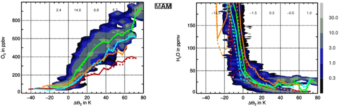
change seriously. Thus, for representativeness, only the O₃ and H₂O distribution for the distance to the 2 PVU surface (4Θ2) for measurements during spring are shown in Fig.6. For the distributions obtained for the other seasons as well as with 4Θ4 as the reference coordinate it is referred toKrebsbach(2005).

The PDFs with respect to the distance to a threshold value of PV look similar to

15

those in the PV space. Anyhow, the use of 4Θ exhibits a slightly more compact shape, in particular for the campaigns in the winter and spring months (see also Sect. 4.3). The fact that the PDFs look very similar in shape and distribution of probabilities in the view of PV and 4Θ suggests an advanced mixing state of these trace gases on surfaces relative to the local tropopause. However, each air parcel in the atmosphere

20

can be thought of as beeing labelled by its PV, controlling or restraining the air parcels’ range of motion. A relatively huge degree of freedom is given in regions of uniform PV

(Sparling and Schoeberl,1995). Thus, spatial gradients of PV might account for the

dynamical affected trace gas distributions and not solely its absolute values. And this is exactly what the PDFs for different PV threshold values for the dynamically defined

25

extra-tropical tropopause show, since the shape and the spreading of distributions re-main to the largest extent the same. This implies that the extra-tropical transition layer follows surfaces of PV or surfaces relative to the shape of the local tropopause, if de-fined by PV, rather than isentropic surfaces. This is consistent with the results ofHoor

ACPD

Print Version Interactive Discussion

EGU

et al. (2004).

4.2. Mixing entropy

A useful measure for the trace gas variability in the PDFs is, for instance, the mixing entropy, which could in general be regarded as a measure for uncertainty. For a uni-modal PDF the characterisation is reliably given by the first and second moments, e.g.

5

mean and variance, respectively. Using these moments, the PDF is described by a relation to a single reference value, like the mean. This is probably inaccurate for a multi-modal distribution, where there is no symmetry around the reference (Sparling,

2000). A measure for the information content in a PDF for a trace gas µ provides Shannon’s entropy which is given as

10 SE = − N X i=1 p_i · l n p_i, (1)

with l n as the natural logarithm (e.g. Srikanth et al., 2000). Concerning a PDF with

D total observed data points of trace gas µ and N bins of width 4µ, the fraction of

observation in the ithcell (p_i) is the number of observations within this cell (N_i) divided by D, andPN

i=1pi = 1. The information content is therefore solely dependent upon a

15

given probability distribution and does not directly relate to the content or meaning of the underlying events, i.e. the quantity of the binned trace gas. Only the probability of the occurring events is important, not the events themselves. SE is zero if the distri-bution has a maximum VMR, e.g. chemical homogeneity within one bin. For a uniform spatial distribution, i.e. p_i=1/N ∀i, the considered trace gas field has a maximum

vari-20

ability (any observed value can be placed in any one of the N bins) and the entropy is maximal (SE=SE_max=ln N). A maximum entropy implies indistinguishability of the air parcels. Moreover, they have an unrestricted free range of motion. In reality, PV constrains the air parcels’ range of motion. Thus, a maximum entropy value is not to be expected (Sparling and Schoeberl,1995). The maximum entropy is dependent upon

ACPD

Print Version Interactive Discussion

EGU

the number of bins. For a better comparison of different entropy values, a normalisation to the maximum entropy is performed, resulting in

SE SE_max = − N X i=1 p_i · l og_N p_i ≤ 1 . (2)

The normalised mixing entropy is illustrated for O₃ and H₂O with PV as the reference coordinate above each seasonal PDF in Fig.5. In the O₃ PDFs the normalised

mix-5

ing entropy values enlarge with an increase in the coordinate value, i.e. height. In the troposphere (i.e. PV values lower than 2 PVU) the normalised mixing entropy is con-siderably small, indicating only small-scale and low trace gas variability. A low mixing entropy value indicates a rather homogeneous air mass. This seems a little bit strange, since a well-mixed state, as an equilibrium state, should have maximum entropy. It

10

should be noted that SE is distinct from the thermodynamical entropy. Thus, the en-tropy here is considered in the “chemical space” in contrast to the “physical space”

(Sparling,2000). The PDFs show highest entropy values in the LMS for O₃and in the

troposphere as well as in the extra-tropical transition layer for H₂O. The corresponding trace gas variability is maximal in these regions, implying the occurrence of different

15

mixing states.

In all used different coordinates, normalised mixing entropy values show a reversed course for O₃ and H₂O (for mixing entropies related to Θ, 4Θ2 and 4Θ4 see

Krebs-bach,2005). Total water mixing ratios are highly variable in the troposphere, whereas ozone is comparably homogeneously distributed with respect to the bin size of the

con-20

sidered coordinate. Due to the strong gradient of both trace gases at or in the vicinity of the tropopause, normalised mixing entropy values increase for O₃and decrease for H₂O with further penetration into the LMS. Therefore, at a PV value of ≈2 PVU also a strong gradient in the normalised mixing entropy is evident. During spring the O₃ vari-ability is highest in the LMS, probably due to the enhanced downward motion. Thus, the

25

O₃entropy values are maximal during this season. The same arises for the enhanced H₂O content and variability in the LMS during the summer months. The seasonal trace

ACPD

Print Version Interactive Discussion

EGU

gas cycles are therefore also reflected by the seasonal course of the mixing entropies. Despite the comprehensive data coverage in the UT/LMS obtained during the SPURT project, it should be mentioned that to derive a more valuable statement from the mixing entropy, considerably more measurements are required, in particular in the upper LMS.

5

4.3. Functional and structural correlations

A common measure for a relation between ordinal or continuous variables is the product-moment coefficient. Pearson’s correlation coefficient (r) reflects the degree of linear relationship between two variables, say x and y, of dimension N. The functional correlation is defined as 10 r_xy = N P i=1 (x_i − ¯x)(y_i − ¯y) s N P i=1 (x_i − ¯x)2 s N P i=1 (y_i − ¯y)2 , (3)

with ¯x ( ¯y) as the mean of the x_i’s (y_i’s). It can range from −1 to +1, inclusive, i.e. from a perfect negative to a perfect positive correlation, whereby r=0 indicates that x and y are uncorrelated. To decide, whether a correlation is significantly stronger than another, Pearson’s r is not an accurate measure, since the individual distributions of x

15

and y are not considered.

A more structural measure for the relationship between two variables provides Spearman’s correlation coefficient (%), which is a non-parametric or rank correlation. The computation is performed by replacing the value of each x_i by the value of its rank, i.e. the smallest value of variable x is converted to rank 1, the highest to rank N. The

20

same applies for the y_i values. An outstanding advantage of the rank correlation is that a non-parametric correlation is more robust than a linear correlation, in the same sense as the median is more robust than the mean (Press et al.,1997). After

convert-ACPD

Print Version Interactive Discussion

EGU

ing the numbers to ranks the Spearman correlation coefficient is calculated according to Eq. (3).

In Table1both Pearson’s and Spearman’s correlation coefficients are shown for O₃ (top) versus different parameters. Ozone does not show best correlations with potential temperature. As is directly evident from both coefficients, highest positive correlations

5

appear when O₃ is related to PV and/or to 4Θ. The coefficients are also high for al-most all chosen PV threshold values to define the local dynamical tropopause. Further, this rather simple measure for the association between two parameters reveal the con-clusion drawn from the PDFs. Trace gas isopleths of O₃seem to be orientated along surfaces of PV rather than along isentropes. The differences between r and % for PV

10

and the 4Θs are only small. In contrast, the correlations of O3with pressure are com-paratively insignificant, nevertheless exhibiting larger structural negative coefficients during some winter and spring campaigns.

The correlation coefficients for H2O versus different parameters are listed in Table1

(bottom). When calculating Pearson’s r, H₂O is best correlated with pressure. Both,

15

p and H₂O, decrease very rapidly with height in a rather logarithmic manner. Thus,

the good correlation is to be expected. This is especially evident during the summer campaigns (IOP 4 and IOP 8). Spearman’s % is independent on the mode or shape of the distribution, and it renders unnecessary to make assumptions on the functional relationship (Press et al.,1997). For this measure, H₂O shows, as O₃, a high degree

20

of correlation when related toΘ, 4Θ and PV.

5. Conclusions

The unique, continuous and high resolution O₃and H₂O measurements, obtained dur-ing the SPURT campaigns between November 2001 and July 2003, allow for a compre-hensive view of the UT/LMS region above Europe. In the first part, seasonal cycles of

25

O₃ and H₂O in the UT and LMS have been analysed. As indicated by extensive stud-ies of vertical profiles obtained during ascents and descents (see Hoor et al.,2004;

ACPD

Print Version Interactive Discussion

EGU

Krebsbach,2005), the tropopause location, i.e. the noticeable boundary between the

troposphere and the stratosphere, coincides quite well with the 2 PVU surface. Di ffer-ent analyses of the trace gas measuremffer-ents reveal that the seasonal cycle of O₃in the UT shows a spring to summer maximum, most probably affected by in situ photochem-istry (cf. also Hegglin et al.). In the LMS the seasonal O₃ cycle is more pronounced

5

and shifted in phase by about 2–3 months earlier in the year, exhibiting a distinct spring time maximum. In the upper part of the LMS, a pronounced O₃maximum is established during spring, whereas the lower part of the LMS still contains large contributions of rather O₃-poor tropospheric air during winter and early spring. Only around April the O₃ maximum is also established in the lower part. This is the effect of the large-scale

10

stratospheric winter/spring Brewer-Dobson circulation (see also Krebsbach et al., a, and Hegglin et al.). Induced by breaking Rossby waves and strong diabatic subsidence (the downward control principle, Haynes et al.,1991) aged and O₃-rich stratospheric air is transported downward into the LMS (e.g.Austin and Follows, 1991;Beekmann

et al.,1994;Logan,1999). Thus, during spring a contribution of stratospheric O₃due

15

to stratosphere-to-troposphere transport is likely to affect tropospheric O3.

In contrast to the O₃seasonal cycles, H₂O shows no phase shift between the UT and the LMS. Maximum H₂O VMRs were observed during the summer campaigns close to the tropopause in the UT as well as in the LMS. Lowest H₂O VMRs were measured dur-ing winter and autumn, the latter indicatdur-ing a temporally link with the sub-tropics/tropics

20

(cf. Krebsbach et al., a, b). The reason for this seasonality is twofold. First, since H₂O is strongly influenced by heterogeneous processes, it follows the temperature variation at the tropopause, i.e. the air is widely freeze-dried during its transport into the LMS (see also Krebsbach et al., c). Second, whereas downward transport of dry air from the overworld into the LMS is dominant during winter, the barrier for quasi-isentropic

25

transport of moist air over the tropopause deep into the LMS is weak during summer. To examine the distribution, spreading, and variability of both trace gases, especially 2-dimensional probability distribution functions were used. Moreover, from these distri-butions, effects of transport and mixing processes can be inferred. Considering several

ACPD

Print Version Interactive Discussion

EGU

chemical, thermal, and dynamical coordinates, the measured trace gases show most compact distributions and best correlations when related to potential vorticity and dis-tance to the dynamically defined tropopause. Moreover, using various PV threshold values for the extra-tropical tropopause, the distributions show almost the same shape. The trace gas isopleths follow surfaces of PV or the shape of the tropopause, in

accor-5

dance with results fromHoor et al.(2004). This suggests an advanced mixing state on surfaces relative to the shape of the tropopause.

The mixing entropy is assigned to characterise the PDFs and to estimate trace gas variability. Entropy values for O₃ and H₂O in the LMS appear to be maximal during spring and summer, respectively. This indicates highest variability of these trace gases

10

during the respective seasons with greater impact of stratospheric air during spring and tropospheric air during summer.

Acknowledgements. SPURT is an AFO 2000 project and has been funded by the German

BMBF (German: Bundesministerium f ¨ur Bildung und Forschung) under contract No. 07ATF27 and additionally supported by the SNF (Swiss National Fund). The authors acknowledge the

15

ECMWF (European Centre for Medium-Range Weather Forecasts) for usage of meteorological data. We are also grateful to enviscope GmbH (Frankfurt a. M., Germany) for professional tech-nical support and professional organisation. Further thanks are due to the pilots and the GFD (German: Gesellschaft f ¨ur Flugzieldarstellung) for the excellent operation of the Learjet 35A.

References

20

Ancellet, G. and Beekmann, M.: Evidence for changes in the ozone concentrations in the free troposphere over southern France from 1976 to 1995, Atmos. Environ., 31, 2835–2851, 1997. 7254

Appenzeller, C., Holton, J. H., and Rosenlof, K. H.: Seasonal variation of mass transport across the tropopause, J. Geophys. Res., 101, 15 071–15 078, 1996. 7254

25

Austin, J. F. and Follows, M. J.: The ozone record at Payerne: An assessment of the cross-tropopause flux, Atmos. Environ., 25, 1873–1880, 1991. 7255,7268

ACPD

Print Version Interactive Discussion

EGU

Europe and its relation to potential vorticity, J. Geophys. Res., 99, 12 841–12 853, 1994.

7252,7254,7256,7268

Brennikmeijer, C. A. M., Slemr, F., Koeppel, C., Scharffe, D. S., Pupek, M., Lelieveld, J., Crutzen, P., Zahn, A., Sprung, D., Fischer, H., Hermann, M., Reichelt, M., Heintzenberg, J., Schlager, H., Ziereis, H., Schumann, U., Dix, B., Platt, U., Ebinghaus, R., Martinsson, B., Ciais, P.,

Fil-5

ippi, D., Leuenberger, M., Oram, D., Penkett, S., van Velthoven, P., and Waibel, A.: Analyzing Atmospheric Trace Gases and Aerosols Using Passenger Aircraft, EOS, 86, 2005. 7250

Brunner, D., Staehelin, J., and Jeker, D.: Large-Scale Nitrogen Oxide Plumes in the Tropopause Region and Implications for Ozone, Science, 282, 1305–1309, 1998. 7250

Brunner, D., Staehelin, J., Jeker, D., Wernli, H., and Schumann, U.: Nitrogen oxides and ozone

10

in the tropopause region of the Northern Hemisphere: Measurements from commercial air-craft in 1995/1996 and 1997, J. Geophys. Res., 106, 27 673–27 699, 2001. 7254

Chen, P.: Isentropic cross-tropopause mass exchange in the extratropics, J. Geophys. Res., 100, 16 661–16 673, 1995. 7255

Derwent, R. G., Simmonds, P. G., Seuring, S., and Dimmer, C.: Observation and interpretation

15

of the seasonal cycles in the surface concentrations of ozone and carbon monoxide at Mace Head, Ireland from 1990 to 1994, Atmos. Environ., 32, 145–157, 1998. 7254

Dessler, A. E., Hintsa, E. J., Weinstock, E. M., Anderson, J. G., and Chan, K. R.: Mechanisms controlling water vapor in the lower stratosphere: “A tale of two stratospheres”, J. Geophys. Res., 100, 23 167–23 172, 1995. 7257,7258

20

Eluszkiewicz, J.: A three-dimensional view of the stratosphere-to-troposphere exchange in the GFDL SKYHI model, Geophys. Res. Lett., 23, 2489–2492, 1996. 7255

Engel, A., B ¨onisch, H., Brunner, D., Fischer, H., Franke, H., G ¨unther, G., Gurk, C., Hegglin, M., Hoor, P., K ¨onigstedt, R., Krebsbach, M., Maser, R., Parchatka, U., Peter, T., Schell, D., Schiller, C., Schmidt, U., Spelten, N., Szabo, T., Weers, U., Wernli, H., Wetter, T., and Wirth,

25

V.: Highly resolved observations of trace gases in the lowermost stratosphere and upper troposphere from the SPURT project: an overview, Atmos. Chem. Phys. Discuss., 5, 5081– 5126, 2005,

SRef-ID: 1680-7375/acpd/2005-5-5081. 7250,7251

Foot, J. S.: Aircraft measurements of the humidity in the lower stratosphere from 1977 to 1980

30

between 45◦N and 65◦N, Quart. J. Roy. Meteor. Soc., 110, 303–319, 1984. 7257

Good, P. and Pyle, J.: Refinements in the use of equivalent latitude for assimilating sporadic inhomogeneous stratospheric tracer observations, 1: Detecting transport of Pinatubo aerosol

ACPD

Print Version Interactive Discussion

EGU

across a strong vortex edge, Atmos. Chem. Phys., 4, 1823–1836, 2004,

SRef-ID: 1680-7324/acp/2004-4-1823. 7252

Haynes, P. and Shepherd, T.: Report on the SPARC Tropopause Workshop, Bad T ¨olz, Ger-many, 17–21 April 2001, SPARC newsletter N. 17, 2000. 7255

Haynes, P. H., Marks, C. J., McIntyre, M. E., Sheperd, T. G., and Shine, K. P.: On the ”downward

5

control” of extratropical diabatic circulations by eddy-induced mean zonal forces, J. Atmos. Sci., 48, 651–678, 1991. 7268

Hegglin, M. I.: Airborne NO_y-, NO- and O₃-measurements during SPURT: Implications for atmospheric transport, Ph.D. thesis, Swiss Federal Institute of Technology Z ¨urich, Diss. ETH No. 15553, 2004. 7251

10

Hegglin, M. I., Brunner, D., Wernli, H., Schwierz, C., Martius, O., Hoor, P., Fischer, H., Par-chatka, U., Spelten, N., Schiller, C., Krebsbach, M., , Weers, U., Staehelin, J., and Peter, T.: Tracing troposphere-to-stratosphere transport above a mid-latitude deep convective system, Atmos. Chem. Phys., 4, 741–756, sRef-ID: 1680-7324/acp/2004-4-741, 2004,

SRef-ID: 1680-7324/acp/2004-4-741. 7259

15

Hintsa, E. J., Weinstock, E. M., Dessler, A. E., Anderson, J. G., Loewenstein, M., and Podolske, J. R.: SPADE H₂O measurements and the seasonal cycle of stratospheric water vapor, Geophys. Res. Lett., 21, 2559–2562, 1994. 7257

Hintsa, E. J., Boering, K. A., Weinstock, E. M., Anderson, J. G., Gary, B. L., Pfister, L., Daube, B. C., Wofsy, S. C., Loewenstein, M., Podolske, J. R., Margitan, J. J., and Bui, T. P.:

20

Troposhere-to-stratosphere transport in the lowermost stratosphere from measurements of H₂O, CO₂, N₂O and O₃, Geophys. Res. Lett., 25, 2655–2658, 1998. 7258

Hoinka, K. P.: Temperature, Humidity, and Wind at the Global Tropopause, Mon. Wea. Rev., 127, 2248–2265, 1999. 7257

Hollingsworth, A. and L ¨onneberg, P.: The verification of objective analyses: Diagnostics of

25

analysis system performance, Met. Atmos. Phys., 40, 3–27, 1989. 7252

Holton, J. R., Haynes, P. H., McIntyre, M. E., Douglass, A. R., Rood, R. B., and Pfister, L.: Stratosphere-troposphere exchange, Rev. Geophys., 33, 403–439, 1995. 7255,7258

Hoor, P., Gurk, C., Brunner, D., Hegglin, M. I., Wernli, H., and Fischer, H.: Seasonality and extent of extratropical TST derived from in-situ CO measurements during SPURT, Atmos.

30

Chem. Phys., 4, 1427–1442, 2004,

SRef-ID: 1680-7324/acp/2004-4-1427. 7253,7263,7267,7269

ACPD

Print Version Interactive Discussion

EGU 7257

Hoskins, B. J., McIntyre, M. E., and Robertson, A. W.: On the use and significance of isentropic potential vorticity maps, Quart. J. Roy. Meteor. Soc., 111, 877–946, 1985. 7253

Hough, A. M.: Development of a two-dimensional global tropospheric model: Model chemistry, J. Geophys. Res., 96, 7325–7362, 1991. 7254

5

Inamdar, A. K. and Ramanathan, V.: Tropical and global scale interactions among water vapor, atmospheric greenhouse effect, and surface temperature, J. Geophys. Res., 103, 32 177– 32 194, 1998. 7249

Krebsbach, M.: Trace gas transport in the UT/LS: seasonality, stratosphere-troposphere ex-change and implications for the extra-tropical mixing layer derived from airborne O3 and

10

H₂O measurements, Ph.D. thesis, Bergische Universit ¨at Wuppertal, urn:nbn:de:hbz:468-20050180, 2005. 7253,7254,7257,7258,7260,7261,7263,7265,7268

Lindzen, R. S.: Some Coolness Concerning Global Warming, Bull. Am. Met. Soc., 71, 288–299, 1990. 7249

Liu, S. C., Trainer, M., Fehsenfeld, F., Parrish, D., Williams, E. J., Fahey, D. W., H ¨ubler, G., and

15

Murphy, P. C.: Ozone production in the rural troposphere and the implications for regional and global ozone distributions, J. Geophys. Res., 92, 4191–4207, 1987. 7255

Logan, J.: Tropospheric ozone: Seasonal behaviour, trends and anthropogenic influence, J. Geophys. Res., 90, 10 463–10 482, 1985. 7254,7255

Logan, J.: Ozone in rural areas of the United States, J. Geophys. Res., 94, 8511–8532, 1989.

20

7254

Logan, J. A.: An analysis of ozonesonde data for the lower stratosphere: Recommendations for testing models, J. Geophys. Res., 104, 16 151–16 170, 1999. 7254,7255,7268

Marenco, A., V ´alerie, T., N ´ed ´elec, P., Smit, H., Helten, M., Kley, D., Karcher, F., Simon, P., Law, K., Pyle, J., Poschmann, G., von Wrede, R., Hume, C., and Cook, T.: Measurement of ozone

25

and water vapor by Airbus in-service aircraft: The MOZAIC airborne program, An overview, J. Geophys. Res., 103, 25 631–25 642, 1998. 7250

Mastenbrook, H. J. and Oltmans, H. J.: Stratospheric Water Vapor Variability for Washington, DC/Boulder, CO: 1964–82, J. Atmos. Sci., 40, 2157–2165, 1983. 7257

McLinden, C. A., Olsen, S. C., Hannegan, B., Wild, O., Prather, M. J., and Sundet, J.:

Strato-30

spheric ozone in 3-D models: A simple chemistry and the cross-tropopause flux, J. Geophys. Res., 105, 14 653–14 665, 2000. 7249

ACPD

Print Version Interactive Discussion

EGU

Environ., 34, 3545–3561, 2000. 7254

Mottaghy, D.: Ozonmessungen in der unteren Stratosph ¨are, Master’s thesis, Rheinisch-Westf ¨alische Technische Hochschule Aachen, in cooperation with the Institute for Chemistry and Dynamics of the Geosphere, ICG-I: Stratosphere, 2001. 7251

Nedoluha, G. E., Bevilacqua, R. M., Hoppel, K. W., Lumpe, J. D., and Smit, H.: Polar Ozone

5

and Aerosol Measurement III measurements of water vapor in the upper troposphere and lowermost stratosphere, J. Geophys. Res., 107, doi:10.1029/2001JD000 793, 2002. 7249,

7257

Oltmans, S. J. and Hofmann, D. J.: Increase in lower-stratospheric water vapour at a mid-latitude Northern Hemisphere site from 1981 to 1994, Nature, 374, 146–149, 1995. 7257 10

Oltmans, S. J. and Levy II, H.: Surface ozone measurements from a global network, Atmos. Environ., 28, 9–24, 1994. 7255

Pan, L., Solomon, S., Randel, W., Lamarque, J.-F., Hess, P., Gille, J., Chiou, E.-W., and Mc-Cormick, M. P.: Hemispheric asymmetries and seasonal variations of the lowermost strato-spheric water vapor and ozone derived from SAGE II data, J. Geophys. Res., 102, 28 177–

15

28 184, 1997. 7249,7255,7257,7258

Pan, L. L., Hintsa, E. J., Stone, E. M., Weinstock, E. M., and Randel, W. J.: The seasonal cycle of water vapor and saturation vapor mixing ratio in the extratropical lowermost stratosphere, J. Geophys. Res., 105, 26 519–26 530, 2000. 7249,7258

Park, M., Randel, W. J., Kinnison, D. E., and Gracia, R. R.: Seasonal variation of methane,

20

water vapor, and nitrogen oxides near the tropopause: Satellite observations and model simulations, J. Geophys. Res., 109, doi:10.1029/2003JD003 706, 2004. 7249

Prados, A. I., Nedoluha, G. E., Bevilacqua, R. M., Allen, D. R., Hoppel, K. W., and Marenco, A.: POAM III ozone in the upper troposphere and lowermost stratosphere: Seasonal variability and comparisons to aircraft observations, J. Geophys. Res., 108,

25

doi:10.1029/2002JD002 819, 2003. 7249,7255,7258

Press, W. H., Teukolsky, S. A., Vetterling, W. T., and Flannery, B. P.: Numerical Recipies in Fortran 77: The Art of Scientific Computing, vol. 1 of “Fortran Numerical Recipies”, Press Syndicate of the University of Cambridge, The Pitt Building, Trumpington Street. Cambridge CB2 1RP, 2nd edn., ISBN 0-521-43064-X, 1997. 7266,7267

30

Randel, W. J., Wu, F., Gettelman, A., Russell III, J. M., Zawodny, J. M., and Oltmans, S. J.: Seasonal variation of water vapor in the lower stratosphere observed in Halogen Occultation Experiment data, J. Geophys. Res., 106, 14 313–14 325, 2001. 7249