HAL Id: hal-00330917
https://hal.archives-ouvertes.fr/hal-00330917
Submitted on 23 Aug 2006
HAL is a multi-disciplinary open access
archive for the deposit and dissemination of
sci-entific research documents, whether they are
pub-lished or not. The documents may come from
teaching and research institutions in France or
abroad, or from public or private research centers.
L’archive ouverte pluridisciplinaire HAL, est
destinée au dépôt et à la diffusion de documents
scientifiques de niveau recherche, publiés ou non,
émanant des établissements d’enseignement et de
recherche français ou étrangers, des laboratoires
publics ou privés.
Global diagnostics of the ionospheric perturbations
related to the seismic activity using the VLF radio
signals collected on the DEMETER satellite
O. Molchanov, A. Rozhnoi, M. Solovieva, O. Akentieva, Jean-Jacques
Berthelier, Michel Parrot, François Lefeuvre, P. F. Biagi, L. Castellana, M.
Hayakawa
To cite this version:
O. Molchanov, A. Rozhnoi, M. Solovieva, O. Akentieva, Jean-Jacques Berthelier, et al.. Global
di-agnostics of the ionospheric perturbations related to the seismic activity using the VLF radio signals
collected on the DEMETER satellite. Natural Hazards and Earth System Science, Copernicus
Publi-cations on behalf of the European Geosciences Union, 2006, 6 (5), pp.745-753. �hal-00330917�
Nat. Hazards Earth Syst. Sci., 6, 745–753, 2006 www.nat-hazards-earth-syst-sci.net/6/745/2006/ © Author(s) 2006. This work is licensed under a Creative Commons License.
Natural Hazards
and Earth
System Sciences
Global diagnostics of the ionospheric perturbations related to the
seismic activity using the VLF radio signals collected on the
DEMETER satellite
O. Molchanov1, A. Rozhnoi1, M. Solovieva1, O. Akentieva2, J. J. Berthelier3, M. Parrot4, F. Lefeuvre4, P. F. Biagi5, L. Castellana5, and M. Hayakawa6
1Institute of the Earth Physics, RAS, Moscow, Russia 2Institute of Space Research, RAS, Moscow, Russia 3Institute CETP, Paris, France
4LPCE/CNRS, Orleans, France
5Department of Physics, University of Bari, Bari, Italy 6University of Electro-Communications, Chofu-Tokyo, Japan
Received: 12 July 2006 – Revised: 22 August 2006 – Accepted: 22 August 2006 – Published: 23 August 2006
Abstract. The analysis of the VLF signals radiated by ground transmitters and received on board of the French DEMETER satellite, reveals a drop of the signals (scat-tering spot) connected with the occurrence of large earth-quakes. The extension of the “scattering spots” zone is large enough (1000–5000 km) and, probably, it increases with the magnitude of the “relative” earthquake. A possible model to explain the phenomenology, based on the acoustic grav-ity waves and the ionosphere turbulence, is proposed. The method of diagnostics applied to this study has the advan-tage to be a global one due to the world wide location of the powerful VLF transmitters and of the satellite reception. However, a specific disadvantage exists because the method requires rather a long time period of analysis due to the large longitudinal displacements among the successive satellite or-bits. At the moment, at least, one month seems to be neces-sary.
1 Introduction
During the last 10–20 years, the disturbances of the iono-sphere related to the seismic activity attracted noticeable at-tention keeping in mind possibilities to use them both for the earthquake forecast and for studying the lithospheionosphere coupling. There are two directions of the re-searches in this field as it will be explained in the following.
Correspondence to: P. F. Biagi
The first one is the observation in situ, i.e. on board satel-lites, of the disturbances. Several papers have been pub-lished on such topic (Parrot et al., 1993; Hayakawa, 1997; Molchanov et al., 2002). However, the satellite observations are not so easy to be accepted. The previous papers were useful for triggering the attention on the phenomenon, but they are controversial because generally no way exists to re-ject the hypotheses of pure coincidences taking into account the possibility of many internal ionosphere instabilities. The statistical studies seem to be obviously more reliable, but the results are partial ones and difficult to compare because of some difference in the sensors used (electric or/and magnetic sensors), in the sensor sensitivities, in the data selection, in the parameters to extract, in the way to estimate them and the validity tests. The actual controversies on the interpretation of the statistical studies performed by several low altitude satellites, are related to the quoted problems. Nevertheless, recent papers have shown that weak but reliable changes in the ionospheric plasma turbulence appear around (±7 days) the occurrence of large earthquake. Its intensity decreases for spatial scales of tenths-hundreds kilometers and it increases for scales of hundred meters (Molchanov et al., 2004; Hobara et al., 2005).
The second research direction is the far distant remote sounding of the ionospheric perturbations related to the seis-mic activity by means of electromagnetic signals. Many results have been published on sounding in UHF fre-quency range (F∼ GHz) by GPS signals (Liu, 2001), on HF sounding (F∼0.5–20 MHZ) from the ground-based or satellite-based ionospheric sondes (Liperovsky et al., 2000; Pulinets, 1998), on LF sounding (F∼200 kHz) from the
746 O. Molchanov et al.: VLF signals collected by DEMETER satellite
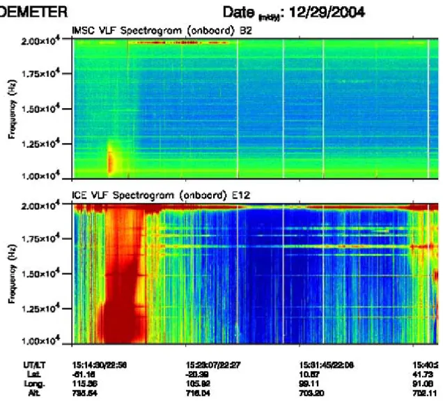
Fig. 1. An example of registration in the 10–20 kHz range during one orbit of the satellite on 29 December 2004. Dynamic spectra of magnetic component (above) and electric component (below) together with orbital data on universal/local time (UT/LT), latitude, longitude and altitude (km) along the orbit. The horizontal lines are the signals from the VLF transmitters. The lines at F=11.90 kHz, F=12.64 kHz and F=14.88 kHz are the signals of the Russian system RSND (A1, A2and A3in Table 1), but the strongest signals at F=19.8 kHz come from
the Australian NWC transmitter.
Table 1. Characteristics of some VLF transmitters.
Frequency (kHz) Code Place of transmitter Longitude Latitude 11.9; 12.64; 14.88 A1 Krasnodar, Russia 38.39 45.02 11.9; 12.64; 14.88 A2 Novosibirsk, Russia 82.58 55.04 11.9; 12.64; 14.88 A3 Komsomolsk Na Amure, Russia 136.58 50.34
16.56 DFY Germany 13.0 52.5
17.8 JP Southern Japan ∼130 ∼32
18.3 FTU Le Blanc, France 1.05 46.37
19.8 NWC North-West Australia 114.08 −21.47
broadcasting transmitters (Biagi et al., 2001, 2004), on VLF sounding (F∼10–40 kHz) from the navigational transmitters (Gufeld et al., 1992; Hayakawa et al., 1996) and on ULF
sounding (F<1 Hz) by magnetospheric magnetic pulsations (Molchanov et al., 2003). Except rather questionable results by satellite topside sounding, all the other ones were obtained
O. Molchanov et al.: VLF signals collected by DEMETER satellite 747
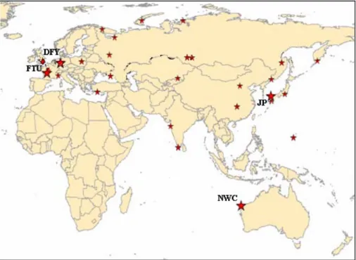
Fig. 2. The stars indicate the location of the powerful VLF transmitters in the eastern hemisphere. The transmitters used in this paper are shown by the larger stars with the indication of their code.
Fig. 3. Evolution of the signal to noise ratio (SNR) values along the orbit on 12 February 2005 at evening (LT∼22.00). The red circle indicates the latitude for which the projection on the ground is at the minimal distance from the VLF transmitter (DFY, 16.56 kHz, in this case). The orbit projection and the color legend is on the right. The reception zones above the transmitter and at the conjugate region in the southern hemisphere are evident.
748 O. Molchanov et al.: VLF signals collected by DEMETER satellite
Fig. 4. The averaged SNR distribution during two months of ob-servation for the NWC transmitter (F=19.8 kHz). The orbits are at day-time (LT∼10 h). In such a case the signal amplitudes and the reception zones are smaller than at night time. Interference parts appear in the region above the transmitter but they are absent in the conjugate area.
by observations on the ground and consequently they were related to more or less local conditions. For example, the reg-istration of VLF radio signals has provided valuable informa-tion on the perturbainforma-tions in the upper atmosphere-lower iono-sphere boundary in an interval of plus/minus several days around the time occurrence of large earthquakes; but the spa-tial area of the analysis was limited to a narrow zone along the path between the transmitter and the receiver (Molchanov and Hayakawa, 1998; Rozhnoi et al., 2004).
Here, the reception on board the DEMETER satellite of the VLF signals radiated by ground transmitters is analyzed. In the past, the reception of such signals was undertaken on many satellites for the investigation of the VLF wave prop-agation and of the interaction with the ionospheric plasma (Aubrey, 1968; Inan and Helliwell, 1982; Molchanov, 1985). The present analysis can be considered as a new method of ionospheric sounding in association with the seismic activity. It was suggested among the perspectives of the DEMETER satellite, whose major scientific objectives are the study of
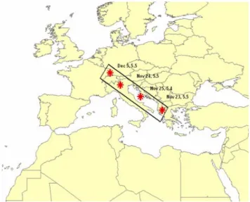
Fig. 5. The stars indicate the location of the earthquakes occurred in Europe during November–December 2004. The relative time oc-currence and magnitude are indicated. The area involved by the seismic activity is approximately indicated with a rectangle.
the ionospheric disturbances in relation to the seismic activ-ity and the definition of the pre and post seismic effects (Par-rot, 2002). The satellite has been launched on 29 June 2004 and its functioning is rather successful.
2 Data analysis
Figure 1 shows an example of satellite VLF electromagnetic registration by both the magnetic field receiver (IMSC) and the electric field receiver (ICE) (Parrot, 2002). In this paper, we will investigate only the electric field data. Frequency res-olution of the spectra is 1F=19.53 Hz and the time averaging is about 2 s. The signals from several powerful VLF ground transmitters are recorded on any orbit. The location in the eastern hemisphere of these VLF transmitters is shown in the Fig. 2. Some characteristics of the transmitters mentioned in this study are listed in Table 1.
The signal to noise ratio (SNR) was computed as follows: SNR = 2A(F0)/[A(F+) +A(F−)]
where A(F0)is the amplitude spectrum density in the fre-quency band including the transmitter frefre-quency F0 and A(F±)are the values outside of the signal band. The choice
of these last values is complicated by the signal spectral broadening in the band F0±δF and by the presence of neigh-boring VLF signals. The spectral broadening is attributed to the VLF signal interaction with the natural ionospheric turbu-lence and it mainly depends on the transmitter power and on the position of the reception point (Bell et al., 1983; Titova et al., 1984; Tanaka et al., 1987). δF usually does not exceed 100 Hz but for powerful transmitters as NWC (19.8 kHz) it
O. Molchanov et al.: VLF signals collected by DEMETER satellite 749
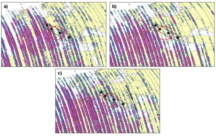
Fig. 6. (a) For the transmitter FTU (18.3 kHz), the SNR distribution averaged during about a month (from 25 October to 22 November 2004) before the earthquakes series. (b) The same as in panel (a), but during/after the earthquakes series (from 23 November to 12 December 2004). (c) The same as in panel (a), but during the period from 26 December 2004 to 31 January 2005, that is after the earthquakes series. The color legend is given in Fig. 4. The red circled area defines roughly the possible “scattering spot” zone.
Fig. 7. Averaged SNR distributions for the DFY transmitter (16.56 kHz): (a) the same as in Fig. 6b, i.e. during/after the earthquakes series, (b) the same as in Fig. 6c, i.e. after the earthquakes series. The color legend is given in Fig. 4. The meaning of the red circled area is the same as in Fig. 6.
can reach the value of 500 Hz. A computation of F±for each
VLF signal and each selected orbit was made by a special procedure. It is based on the analysis of the averaged
back-ground level as function of the difference |F±–F0|. An ex-ample of SNR trend is shown in Fig. 3. The following basic features of the reception zones must be noted: a) the first
750 O. Molchanov et al.: VLF signals collected by DEMETER satellite
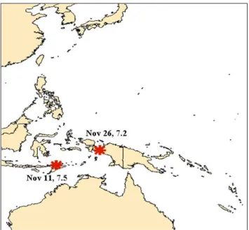
Fig. 8. Map showing the location, magnitude and time occur-rence of the two strong earthquakes happened in Indonesia during November 2004.
reception zone is above the position of the transmitter; b) the second reception zone is in the conjugate area, due to the magnetospheric VLF propagation; c) the near equatorial re-gion is characterized by a disappearance of the signal. Also expected and obvious fast variations of the signal exist and are due to the ionospheric irregularities. In the present study we need to average the signal over the fast variations and try to seek for slow changes in the reception zones during seis-mically active periods.
Generally, two types of ionospheric response to earth-quakes forcing could be assumed. The first is the direct in-fluence of the seismic pulses, which is a co-seismic effect with a duration ranging from several minutes to some hours. The second is a longer indirect response due to some pro-cesses related to earthquakes preparation and post-seismic relaxation, with a duration of days or weeks. By using one satellite a very small chance exists to observe a coseismic effect. A better possibility is the finding of the indirect in-fluence. However, even on this way, the following intrinsic drawback of the satellite observations above a fixed point at the ground, exists: too large longitudinal distances between adjacent orbits (about 2500 km in a case of DEMETER or-bits at the middle latitudes) and day time intervals between orbits above the point in the same local time. So, in order to obtain statistically significant results and a longitudinal spa-tial resolution of 100–200 km, an averaging period of 2–3 weeks, at least, is necessary. It dictates a selection of rather long periods of seismic activity, ad example a series of suc-cessive strong earthquakes. Another problem of the analysis is the incompleteness of the satellite data. However, since the end of October 2004, the data completeness becomes more
than 70%; then, the data are missing from 16 December to 25 December 2004, while the completeness reaches a level of 80–90% since January 2005. The averaged (over a period of 2 months) background variation in the reception zones of the NWC transmitter is shown in the Fig. 4. In the reception zone where the transmitter is located, it can be noted the ap-pearance of interference parts of the VLF modes. This effect does not appear in the conjugate reception zone.
At first, a series of large earthquakes occurred in Eu-rope from 23 November to 5 December 2004 (23 November, M=5.5; 24 November, M=5.5; 25 November, M=5.4; 5 De-cember, M=5.5) were selected. Their epicentres are shown in Fig. 5 and the extent of the area is approximately indi-cated with a rectangle. These earthquakes are rare ones for the large magnitude and the rather short time interval among them. The distribution of the SNR values in the selected area for the signals of the FTU transmitter (F=18.3 kHz) is shown in the Fig. 6 during a period before (from 25 Octo-ber to 22 NovemOcto-ber 2004) the earthquakes series (Fig. 6a), during/after (from 23 November to 12 December 2004) the series (Fig. 6b) and after (26 December 2004 to 31 January 2005) it (Fig. 6c). The missing data period 16–25 December 2004 must be taken into consideration. With this account, the selected three periods of analysis are enough equal in length and adjacent in time. Here and after, only the data for evening orbits are used, because their space reception zone is larger than the day-time orbits ones (Figs. 3 and 4). For the same earthquakes series, the signals of the DFY transmitter (F=16.56 kHz) during/after and after the occurrence of the earthquakes were analysed. Figures 7a and b show the aver-aged distribution of the SNR values in the selected area from 23 November to 12 December 2004 and from 26 December 2004 to 31 January 2005, respectively.
Then, two large earthquakes occurred in Indonesia dur-ing November 2004 (11 November, M=7.5; 26 November, M=7.2) were selected. In Fig. 8, their location, magnitude and occurrence time are indicated. In Fig. 9, the averaged SNR distributions for the JP (17.8 kHz) transmitter during a period before/during (from 30 October to 28 November 2004) the occurrence of the quoted earthquakes (Fig. 9a) and a period after (from 6 January to 7 February 2005) their oc-currence (Fig. 9b), are shown.
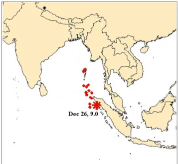
Finally, the Fig. 10 shows the location of the Sumatra big (M=9.0) earthquake on 26 December 2004. The averaged SNR distributions for the NWC (19.8 kHz) transmitter during a period before (from 1 November to 15 December 2004) the occurrence of the quoted earthquake (Fig. 11a) and a period after (from 6 January to 15 February 2005) its occurrence (Fig. 11b), are shown in Fig. 11.
3 Discussion
The data reported in Fig. 6 indicate: a) none definite indica-tion of effects exists (Fig. 6a) before the Europe earthquakes
O. Molchanov et al.: VLF signals collected by DEMETER satellite 751
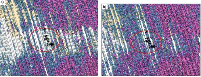
Fig. 9. (a) Averaged SNR distribution for the JP (17.8 kHz) transmitter during the period from 30 October to 28 November 2004, i.e. before and during the time occurrence of the strong earthquakes in Indonesia. (b) The same as in panel (a) but during the period from 6 January to 7 February 2005, i.e. after the occurrence of the earthquakes. The color legend is given in Fig. 4. The red circled areas define roughly the possible “scattering spot” zones.
series on November–December 2004; b) a “scattering spot” seems to appear in the time period which includes the interval of the earthquakes series (Fig. 6b); c) the effect disappears in the period after it (Fig. 6c). For the same earthquakes, the data reported in Fig. 7 confirm the appearance of a “scatter-ing spot” in a period includ“scatter-ing their time occurrence. The data presented in Fig. 9 seem to confirm the results indicated in the previous b) and c) items for the Indonesia earthquakes on November 2004. For the big Sumatra earthquake on De-cember 2004 the data presented in Fig. 11 seem to indicate the appearance of a “scattering spot” before the earthquake occurrence (Fig. 11a). Anyway, since the data period 16–25 December 2004 is missed, this last result is doubtful.
The “scattering spots” have a size of about 1000 km in the case of the earthquakes series in Europe with magni-tude M∼5.5. They are about 2000–3000 km large for the Indonesia earthquakes with M∼7–7.5 and, perhaps, a huge extension of the order of 5000 km, can be considered for the Sumatra earthquake with M=9.0. The previous values are only indicative ones and represent the (greater) extension of the red circled areas reported in the Figs. 6/7, 9 and 11.
The previous results seem to indicate that “scattering spots” in VLF radio signals exist in connection with large earthquakes and their spatial extension increase with the magnitude of the relative earthquake.
The previous long in time and large in extension regions of perturbation in the ionosphere cannot be produced by the seismic shocks itself (duration of minutes/hours). So, it is necessary to suppose some long lasting agent which influ-ences the ionosphere around the time occurrence of a strong earthquake. According to our opinion, the initial agent is an upward energy flux of atmospheric gravity waves (AGW)
Fig. 10. Map showing the location, time occurrence and magnitude of the big Sumatra earthquake on December 2004. The location of other main shocks is also indicated.
which are induced by the gas-water release from the earth-quake preparatory zone (Liperovsky et al., 2000; Molchanov, 2004). The penetration of AGW waves into the ionosphere leads to modification of the natural (background) ionospheric turbulence, especially for space scales ∼1–3 km and wave numbers kT ∼10−4–10−3m−1. Previously, this weak but
re-liable effect was revealed from direct satellite observations (Molchanov et al., 2004; Hobara et al., 2005). Resonant
752 O. Molchanov et al.: VLF signals collected by DEMETER satellite
Fig. 11. (a) Averaged SNR distribution for the NWC (19.8 kHz) transmitter during the period from 1 November to 15 December 2004, i.e. before the occurrence of the Sumatra big earthquake. (b) The same as in panel (a), but during the period from 6 January to 15 February 2005, i.e. after the occurrence of the Sumatra earthquake. The color legend is given in Fig. 4. The red circled area defines roughly the possible “scattering spot” zone.
Fig. 12. Schematic model of the VLF signals scattering assumed to explain the observed effect. AGW indicates the Atmospheric Gravity Waves above the earthquake preparatory zone. The yellow circles represent the modification of the ionospheric turbulence.
scattering of the VLF signals is possible in condition of the frequency- wave number synchronism :
ω0=ωs+ωTk0=ks+kT
where ω0, k0are for the incident VLF wave; ωT, kT are for
the turbulence and ωs, ksare for the scattering waves. It can
be found that the amplitude A0of an incident wave decreases
exponentially during its propagation through the perturbed medium according to the relation:
A0∼=e−αnAtH
where αn is the coefficient of nonlinear interaction, H is
the length of the interaction region and At is the amplitude
of the turbulence. For the VLF signals it is ωT ω0∼ωs,
O. Molchanov et al.: VLF signals collected by DEMETER satellite 753 and the interaction is especially efficient because k0∼ks∼kT
(Molchanov, 1985; Trakhtengertz and Hayakawa, 1993). Therefore, even with a small amplitude AT of the turbulence,
the scattering of the wave could be significant if the length H is large. The Fig. 12 shows a schematic view of the mecha-nism.
4 Conclusions
The method of diagnostics applied on this study has the ad-vantage to be global thanks to the world-wide positioning of the powerful VLF transmitters and to the satellite reception. Anyway, it has the specific disadvantage to require rather long time period of analysis, because the longitudinal dis-tances among the satellite orbits are too large. Above a fixed area, the satellite appears at the same local time only once per day. So, at least one month period of registration is necessary for the longitudinal spacing of about 1000 km.
In any case, this study has revealed the existence of “scattering spots” in VLF radio signals related to large earthquakes and it has approximately defined the size of the perturbed area as function of the earthquake magnitude.
Edited by: M. Contadakis
Reviewed by: C.-V. Meister and another referee
References
Aubrey, M. P.: Six-component observation of VLF signal on FR-1 satellite, J. Atmos. Terr. Phys., 30, 1161–1169, 1968.
Bell, T. F., James, H. G., Inan, U. S., and Katsufrakis, J. P.: The apparent spectral broadening of VLF transmitter signals during transionospheric propagation, J. Geophys. Res., 88, 4813–4816, 1983.
Biagi, P. F., Piccolo, R., Ermini, A., Martellucci, S., Bellecci, C., Hayakawa, M., Capozzi, V., and Kingsley, S. P.: Possible earth-quake precursors revealed by LF radio signals, Nat. Hazards Earth Syst. Sci., 1, 99–104, 2001,
http://www.nat-hazards-earth-syst-sci.net/1/99/2001/.
Biagi, P. F., Piccolo, R., Castellana, L., Ermini, A., Martellucci, S., Bellecci, C., Capozzi, V., Perna, G., Molchanov, O., and Hayakawa, M.: Variations in a LF radio signal on the occasion of the recent seismic and volcanic activity in Southern Italy, Phys. Chem. Earth, 29, 551–557, 2004.
Gufeld, I. L., Rozhnoi, A. A., Tyumensev, S. N., Sherstuk, S. V., and Yampolsky, V. S.: Radiowave disturbances in period to Rudber and Rachinsk earthquakes, Phys. Solid Earth, 28(3), 267–270, 1992.
Hayakawa, M.: Electromagnetic Precursors of Earthquakes: Re-view of Recent Activities, Rev. Radio Sci., 1993–1995, Oxford Univ. Press, 807–818, 1997.
Hayakawa, M., Molchanov, O. A., Ondoh, T., and Kawai, E.: The precursory signature effect of the Kobe earthquake on subiono-spheric VLF signals, J. Comm. Res. Lab., 43, 169–180, 1996. Hobara, Y., Lefeuvre, F., Parrot, M., and Molchanov, O. A.: Low
latitude ionospheric turbulence and possible association with
seismicity from satellite Aureol 3 data, Ann. Geophys., 23, 1259–1270, 2005,
http://www.ann-geophys.net/23/1259/2005/.
Inan, U. S. and Helliwell, R. A.: DE-1 observations of VLF transmitter signals and wave-particle interaction in the magne-tosphere, Geophys. Res. Lett., 9, 917–923, 1982.
Liperovsky, V. A., Pokhotelov, O. A., Liperovskaya, E. V., Parrot, M., Meister, C.-V., and Alimov, O. A.: Modification of sporadic E-layers caused by seismic activity, Surveys in Geophysics, 21, 449–486, 2000.
Liu, J. Y., Chuo, Y. J., and Chen, Y. I.: Ionospheric GPS TEC per-turbations prior to the 20 September 1999, Chi-Chi earthquake, Geophys. Res. Lett., 28, 1383–1386, 2001.
Molchanov, O. A.: VLF waves and induced emissions in the near-Earth plasma, Moscow, Nauka, 223 pp, 1985.
Molchanov, O. A.: On the origin of low- and middle-latitude iono-spheric turbulence, Phys. Chem. Earth, 29, 559–567, 2004. Molchanov, O. A, Hayakawa, M., Afonin, V. V., Akentieva, O. A.,
and Mareev, E. A.: Possible influence of seismicity by grav-ity waves on ionospheric equatorial anomaly from data of IK-24 satellite1. Search for idea of seismo-ionosphere coupling, in: Seismo-Electromagnetics (Lithosphere-Atmosphere-Ionosphere Coupling), edited by: Hayakawa, M. and Molchanov, O., TER-RAPUB, 275–285, 2002.
Molchanov, O. A., Schekotov, A. Y., Fedorov, E. N., Belyev, G. G., and Gordeev, E. I.: Preseismic ULF electromagnetic effect from observation at Kamchatka, Nat. Hazards Earth Syst. Sci., 3, 203– 209, 2003,
http://www.nat-hazards-earth-syst-sci.net/3/203/2003/.
Molchanov, O. A., Akentieva, O. S., Afonin, V. V., Mareev, E. A., and Fedorov, E. N.: Plasma density-electric field turbulence in the low-latitude ionosphere from the observation on satellites; possible connection with seismicity, Phys. Chem. Earth, 29, 569– 577, 2004.
Parrot, M.: The micro-satellite DEMETER: data registration and data processing, in: Seismo-Electromagnetics (Lithosphere-Atmosphere-Ionosphere Coupling), edited by: Hayakawa, M. and Molchanov, O., TERRAPUB, 660–670, 2002.
Parrot, M., Achache, J., Berthelier, J. J., Blanc, E., Deschamps, A., Lefeuvre, F., Menvielle, M., Planet, J. L., Tarits, P., and Villain, J. P.: High-frequency seismo-electromagnetic effects, Phys. Earth Planet. Inter., 77, 65–83, 1993.
Pulinets, S. A.: Seismic activity as a source of the ionospheric vari-ability, Adv. Space Res., 22, 903–906, 1998.
Rozhnoi, A., Solovieva, M. S., Molchanov, O. A., and Hayakawa, M.: Middle latitude LF (40 kHz) phase variations associated with earthquakes for quiet and disturbed geomagnetic conditions, Phys. Chem. Earth, 29, 589–598, 2004.
Tanaka, Y., Lagoutte, D., Hayakawa, M., and Lefeuvre, F.: Spectral broadening of VLF transmitter signals and sideband structure ob-served on Aureol-3 satellite at middle latitudes, J. Geophys. Res., 92, 7551–7559, 1987.
Titova, E. E., Di, V. L., and Jurov, V. E.: Interaction between VLF waves and the turbulent ionosphere, Geophys. Res. Lett., 11, 323–330, 1984.
Trakhtengerts, V. Y. and Hayakawa, M.: A wave-wave interaction in whistler frequency range in space plasma, J. Geophys. Res., 98, 19 205–19 217, 1993.