HAL Id: hal-00298291
https://hal.archives-ouvertes.fr/hal-00298291
Submitted on 5 Oct 2006
HAL is a multi-disciplinary open access
archive for the deposit and dissemination of
sci-entific research documents, whether they are
pub-lished or not. The documents may come from
teaching and research institutions in France or
abroad, or from public or private research centers.
L’archive ouverte pluridisciplinaire HAL, est
destinée au dépôt et à la diffusion de documents
scientifiques de niveau recherche, publiés ou non,
émanant des établissements d’enseignement et de
recherche français ou étrangers, des laboratoires
publics ou privés.
ecosystem model using SOFA: setup and identical twin
experiments
G. Crispi, M. Pacciaroni, D. Viezzoli
To cite this version:
G. Crispi, M. Pacciaroni, D. Viezzoli. Simulating biomass assimilation in a Mediterranean ecosystem
model using SOFA: setup and identical twin experiments. Ocean Science, European Geosciences
Union, 2006, 2 (2), pp.123-136. �hal-00298291�
www.ocean-sci.net/2/123/2006/
© Author(s) 2006. This work is licensed under a Creative Commons License.
Ocean Science
Simulating biomass assimilation in a Mediterranean ecosystem
model using SOFA: setup and identical twin experiments
G. Crispi, M. Pacciaroni, and D. Viezzoli
Istituto Nazionale di Oceanografia e di Geofisica Sperimentale, Trieste, Italy Received: 31 March 2006 – Published in Ocean Sci. Discuss.: 19 June 2006
Revised: 14 September 2006 – Accepted: 29 September 2006 – Published: 5 October 2006
Abstract. Assessing the potential improvement of basin scale ecosystem forecasting for the Mediterranean Sea re-quires biochemical data assimilation techniques. To this aim, a feasibility study of surface biomass assimilation is performed following an identical twin experiment approach. NPZD ecosystem data generator, embedded in one eighth degree general circulation model, is integrated with the reduced-order optimal interpolation System for Ocean Fore-casting and Analysis.
The synthetic “sea-truth” data are winter daily averages obtained from the control run (CR). The twin experiments consist in performing two runs: the free run (FR) with summer-depleted phytoplankton initial conditions and the as-similated run (AR), in which, starting from the same FR phy-toplankton concentrations, weekly surface biomasses aver-aged from the CR data are assimilated. The FR and AR initial conditions modify the winter bloom state of the phytoplank-ton all over the basin and reduce the total nitrogen, i.e. the energy of the biochemical ecosystem.
The results of this feasibility study shows good perfor-mance of the system in the case of phytoplankton, zooplank-ton, detritus and surface inorganic nitrogen. The weak results in the case of basin inorganic nitrogen and total nitrogen, the latter nonperformant at surface, are discussed.
1 Introduction
The last two decades of the twentieth century saw the de-velopment of remote sensing techniques to study the distri-bution of phytoplankton in the ocean. This technology uses subtle variations in the color of the oceans, as monitored by a sensor aboard satellites, to quantify the concentrations of chlorophyll-a in the surface layers of the ocean. Since
polar-Correspondence to: G. Crispi
orbiting satellites’ swaths cover the globe at high spatial res-olution – 1 km or better, it is possible to see in great wealth of detail the variations in phytoplankton distribution at syn-optic scales (Gordon and Morel, 1983). On this innovations are based the improvements of models describing photosyn-thesis as a function of available light.
The aim of this work is to evaluate the feasibility, the efficiency and the limits of the assimilation of superficial biomass data in view of possible activities in operational oceanography. The framework relies on Observing System Simulation Experiment (OSSE). OSSEs are used for two dis-tinct objectives: to define the best observational network for improving forecasting; to determine the impact of an hypo-thetical dataset upon a simulated system. The result of the OSSE is in both cases the measure of the distance of the ecosystem evolving with or without the data network un-der analysis (Raicich, 2006; Vecchi and Harrison, 2006). This kind of methodology has been performed by means of the singular evolutive extended Kalman filter and of the ensemble variant of this method respectively in the one-dimensional ecosystem model and in the three-one-dimensional one of the Cretan Sea (Triantafyllou et al., 2005).
The OSSE here proposed provides a preliminary quanti-tative basis for assessing the impact of a synthetical data network of surface biomass on a Mediterranean simulated ecosystem. The methodology of identical twin experiments (ITE) is chosen for understanding the surface biomass data impact on the ecosystem, taking into account the knowledge of the biomass coverage all over the basin.
Synthetic “sea-truth” data are generated by a control run for assimilation in the ITE. The twin experiments consist in a free run with some modified conditions (initial conditions, parameters of the model, forcing functions, etc.) with re-spect to the control run and an assimilated simulation, with the same modified conditions of the free, assimilating in ad-dition the data extracted from the control run according to the network design. With this numerical experiment we want
to study times and paths of the recovery of the initial states under biomass assimilation after reducing the biochemical energy at disposal of the ecosystem, i.e. in more oligotrophic conditions.
Along the vertical dimension, two levels are chosen for a total of 20 m from the sea surface. This is understandable from the point of view of detectability in analogy with the penetration optical length in the Mediterranean.
The choice of the biomass as proxy of the chlorophyll should suggest that identical values are chosen at all the top layers. We choose a more realistic procedure starting from the fact that the ecological phytoplankton variable is dependent on the specific depths. This maintains its validity when chlorophyll corrections are introduced in an ecosystem model instead of biomass, with one single average concentra-tion at each posiconcentra-tion. In fact the tranformaconcentra-tion of the chloro-phyll data into biomass requires a transformation parameter: the carbon:chlorophyll ratio.
This parameter can be analytical, statistical or dynamical. It has the following dependences: limiting nutrient, tempera-ture and photosynthetic available radiation (PAR). Therefore, it depends in general on the vertical dimension implicitly in the first two parameters, and explicitly in the last one, the PAR. In this ITE the dependence is “forced” at the time of in-troducing the surface biomass in the system, with one value at 5 m and another at 15 m. The error of the measurement plus the transformation is taken as constant, and the latter is supposed unbiased.
The procedure which can meet the most success relies on models of the photosynthesis as a function of the PAR and of the nutrient cycling. Thus the light available at the sea surface is estimated in this work using optimization meth-ods, and the nitrogen limitation is traced as discussed in the following section.
The numerical experiments are based upon an established ecosystem model setup in the frame of the European Com-mission Mediterranean Targeted Projects 1 (Pinardi et al., 1997) and 2 (Monaco and Peruzzi, 2002). The model has moderate biochemical complexity to be used in tight cou-pling with the assimilation scheme. Moreover there is expe-rience that such a modelling approach can capture the main biogeochemical fluxes characteristics of the Mediterranean basin: oligotrophy, seasonal cycle, biological gradients (Civ-itarese et al., 1996).
In the following section the integrated system setup is out-lined. The dynamical adjustment of the initial conditions is considered in the third section, while in the fourth one the results in terms of overall content in the different ecosystem compartments and their statistics are shown. The last section reports the conclusions.
2 Ecological model setup
The dynamic of the Mediterranean oligotrophic ecosystem is studied through coupling with the Mediterranean basin circu-lation as simulated by a General Circucircu-lation Model (GCM) driven by high frequency forcing. Consistently, an ecosystem description considering the general three-dimensional circu-lation has been set up and embedded in the GFDL-MOM im-plemented in the Mediterranean Forecasting System Project (Demirov and Pinardi, 2002).
The simulations reported here adopt a GCM for the Mediterranean Sea plus a buffer zone representing the At-lantic inflow/outflow. The biharmonic horizontal eddy vis-cosity is 0.5 1018cm4s−1 and the biharmonic horizontal
eddy diffusivity is 1.5 1018cm4s−1for physical tracers. The
vertical viscosity is 1.5 cm2s−1, the vertical diffusivity for
temperature and salinity is 0.3 cm2s−1.
The specification of salt fluxes at surface is obtained with the relaxation of model sea surface salinity toward climato-logical casts for the Mediterranean area. Convective adjust-ment is performed mixing, up to nC times, the contents of two adjacent vertical levels, when static instability occurs.
Air-sea physical parameterizations account for the heat budget at the air-sea interface using sea surface temperature prognosed by the model and six-hourly atmospheric fields from European Center for Medium-Range Weather Forecast – ECMWF.
The identical twin experiments start from the final con-ditions of the dynamical adjustment stage, spanning from 1 September to 28 December. The same conditions initial-ize the control run (CR), which generates the daily averaged phytoplankton at 5 m and 15 m to be assimilated in the ITE after weekly averages.
The identical twin experiments start on 29 December and, after reaching the end of the year, they continue adopting the 1 January till the 7 March forcings of the same 1998 repeat-ing year, see Fig. 1. They are run under conditions, eco-logical parameters and forcing functions identical to the CR ones.
The free run (FR) is reinitialized to the phytoplankton summer initial conditions and no assimilation is performed. The assimilated run (AR) starts from the phytoplankton sum-mer initial conditions of the free run and the weekly data of phytoplankton, as averaged from the daily results of the con-trol run, are assimilated at the end of each week.
The model is integrated throughout all the Mediterranean basin, with horizontal spatial discretization of one eighth de-gree and with vertical resolution of 31 levels. On the same grid the equations describing nitrogen uptake, grazing and remineralization processes, are integrated. The vertical levels are unevenly spaced down to bottom, and the tracer values, temperature, salinity and biochemical ones, biomass among the others, are placed at 5, 15, 30, 50, 70, 90, 120, 160, 200, 240, 280, 320, 360, 400, 440, 480, 520, 580, 660, 775,
925, 1150, 1450, 1750, 2050, 2350, 2650, 2950, 3250, 3550, 3850 m.
The generic NPZD ecosystem model is based on nitrogen units. Firstly, a reciprocal interaction between the elemental composition of marine biota and their dissolved nutrition re-sources is assumed, whereby the nutrient elements are taken up and released in fixed proportions of C:N:P of 106:16:1 (Redfield et al., 1963). Secondly, the biological production is principally limited by the availability of nitrogen, meaning that the supply of nitrogen also determines the amount of car-bon incorporated into biomass. Production based on nitrogen (e.g. nitrate), which newly enters the euphotic zone, where light availability is sufficient for net growth, is referred to as new production and is differentiated from production based on the remineralized compounds of nitrogen. Accordingly, the export flux of organic material from this upper oceanic layer equals the new production.
The basic equations of the NPZD model are presented in the following, and the diagram flux is shown in Fig. 2. The three-dimensional coupling of generic equation of the bio-logical tracer B with sea velocity field u=(u, v, w) is:
∂B ∂t +(u · ∇)B = −KH∇ 4 HB + KV ∂2B ∂z2 −wB∂B∂z + ∂B∂t SOURCE
with hydrodynamics and its parameterization on the same grid of the Mediterranean circulation model, where the equa-tions describing nitrogen uptake, grazing and remineraliza-tion processes, are integrated. Each variable has a posi-tive flux to the following ones: the uptake from inorganic nitrogen to phytoplankton; the grazing from phytoplankton to zooplankton; the mortality from zooplankton to detritus; and the remineralization from detritus to inorganic nitrogen. Also the specific mortality from phytoplankton to detritus is shown in Fig. 2. These five fundamental fluxes are completed by the cross fluxes from zooplankton to inorganic nitrogen, the excretion, and from phytoplankton to detritus, the sloppy feeding.
Biogeochemical equations, without any recourse to boundary conditions inside the integration domain, are solved in an insulating, conservative way through second-order finite difference method, on the numerical Arakawa B-grid, at the timestep of 900 s. When instabilities occur in the biogeochemistry, biological sources and sinks are set to zero and the calculations proceed after borrowing.
The nitrogen model represents the space and time evolu-tion of nitrate, N, phytoplankton, P, zooplankton, Z, detri-tus, D, each expressed in nitrogen units. The phytoplankton equation is given by the following expression:
∂P ∂t SOURCE =G(t ) N P kN+N −d P − γ P Z kP +P
Growth limitation, G(t), is described by the Eppley (1972) function:
Fig. 1. OSSE strategy and assimilated data generator. The GCM
physical variability spans in the twin numerical experiments the same period from 29 December to 7 March using u and v wind ve-locity components and total cloud coverage, and turning the winter conditions of the phytoplankton into summer initial values.
Fig. 2. Diagram of the nitrogen fluxes linking the biochemical
com-partments NPZD.
G(t ) = Gmaxe−kTTE(I, Iopt, z, t )with
E(I, Iopt, z, t ) = p(t )
I Iopt
e1−(I /Iopt)
Here the limitation by photosynthetic available radiation is given in terms of the photoperiod in the julian day, p(t), of the Ioptoptimum light irradiance, and of the PAR, I, at z depth:
Fig. 3. Inorganic nitrogen initial vertical profile in the
Mediter-ranean Sea and inorganic nitrogen restoration profiles in the Atlantic buffer box and in the Adriatic and Aegean marginal seas. Phyto-plankton and zooPhyto-plankton initial profiles are given in the inner plate with the same units (µmol N dm−3).
expressed as function of the irradiance at surface, I0(t),
op-timized following data by Sverdrup at al. (1942) using the Lambert-Beer light extinction law.
Grazing activity is expressed in order to introduce sloppy feeding and excretion:
∂Z ∂t SOURCE =ηγ P Z kP +P −δ Z
The inorganic nitrogen takes into account all the other bio-chemical variables as follows:
∂N ∂t SOURCE =r D + (1 − α)δ Z − G N P kN+N
The detritus chain describes the remaining part of the bio-geochemical cycles of carbon and macronutrients, that is the recycling, through mineralization, of the nonliving organic matter, particulate and dissolved, produced by exogenous in-put, mortality processes, excretion and exudation, all set as linear processes. The introduction of the detritus compart-ment permits to follow the fate and the remineralization of the particulate matter at a basin and sub-basin scale below
the euphotic zone, which are conditions for balancing the new production: ∂D ∂t SOURCE =d P + (1 − η)γ P Z kP +P +α δ Z − r D
All the parameters are chosen in literature ranges for olig-otrophic environments (Table 1). This enables to calibrate, considering selected results from MTP I and MTP II Projects, the 3-D model to the values of detritus remineralization and sinking.
The version 3.0 of System for Ocean Forecast and Analy-sis (SOFA) by De Mey and Benkiran (2002) is used for as-similating surface biomass data. This reduced-order optimal interpolation system operates under the condition that the background analysis error matrix is calculated from the back-ground error variances, calculated from the previous analy-sis error variances, and from the correlations, estimated on the observational data and taken fixed during the simula-tion. Thus SOFA evaluates directly the horizontal correla-tions at observation locacorrela-tions, assuming them vertically un-correlated. The observational error covariance matrix is diag-onal and the parameters for these twin experiments are given in Table 2.
SOFA, using temperature and salinity as tracers (Raicich and Rampazzo, 2003), has been integrated with the NPZD-based ecosystem model. After optimization on SP4, the in-tegrated system execution time is reduced approximately by three, from about 600 to 227 s for one day simulation with time-step of 900 s.
3 Dynamical adjustment of initial conditions
Phytoplankton initial conditions are chosen from the data of an averaged summer profile. Averaged biomass stations were measured by Berland et al. (1988; Fig. 5) in the Balearic Sea, in the Ionian Sea and in the Levantine. A ratio of 0.05 for estimating the chlorophyll to carbon is used. The profile is shown in Fig. 3, inner panel. Zooplankton is initialized as one ninth of the phytoplankton value, i.e. around 11–12% of the total phytoplankton content.
Mean nitrate summer conditions are extracted from the MEDAR climatology (Manca et al., 2004). Southern Balearic (DS4), northern Ionian (DJ7) and Cretan Passage (DH3) areas are selected and averaged, in correspondence to the stations in which phytoplankton data were acquired. The interpolation at the levels of the model is shown in Fig. 3, large panel (diamonds). This profile initializes nitrate vari-able for all the Mediterranean basin.
Atlantic Ocean and marginal seas, Adriatic and Aegean, influences upon the pelagic Mediterranean Sea are treated using historical data (Fig. 3) at which these three buffer boxes are relaxed during all the simulations, with αB restoration time.
Table 1. List of the biochemical parameters.
Parameter Definition Value
η Zooplankton efficiency 0.75
α Degradation fraction 0.33
γ Zooplankton growth 1.157 10−5s−1
δ Zooplankton mortality 1.730 10−6s−1 kP Grazing half-saturation 1.0 µmol N dm−3
r Detritus remineralization rate 1.18 10−6s−1 kN Nitrate half-saturation 0.25 µmol N dm−3 Gmax Maximum growth rate 6.83 10−6s−1 kT Temperature coefficient 6.33 10−20C−1 d Phytoplankton mortality 5.55 10−7s−1 KH Horizontal turbulent diffusion 1.5 1018cm4s−1
KV Vertical turbulent diffusion 1.5 cm2s−1
kz Light extinction coefficient 0.00034 cm−1
Iopt/I0 Optimum light ratio 0.5 nC Cox turbulence iteration number 10
αB Newtonian restoration time 1.0 day−1
wB Sinking for the N, P, Z, D tracers 0, 0, 0, 0.0058 cm s−1
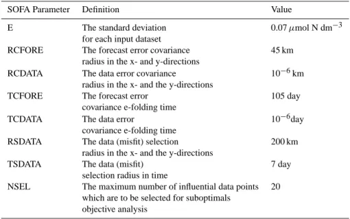
Table 2. List of the SOFA parameters.
SOFA Parameter Definition Value
E The standard deviation 0.07 µmol N dm−3 for each input dataset
RCFORE The forecast error covariance 45 km radius in the x- and y-directions
RCDATA The data error covariance 10−6km radius in the x- and the y-directions
TCFORE The forecast error 105 day covariance e-folding time
TCDATA The data error 10−6day covariance e-folding time
RSDATA The data (misfit) selection 200 km radius in the x- and the y-directions
TSDATA The data (misfit) 7 day selection radius in time
NSEL The maximum number of influential data points 20 which are to be selected for suboptimals
objective analysis
The Atlantic station data are selected from the ATLANTIS II cruise report (Osborne et al., 1992). The reference latitude is 36.5◦N and the longitude of these casts range from 9.5◦W to 8◦W. Atlantic and Gibraltar restoring condition are im-posed to the subbasin from 9.25◦W to 6◦W.
For the Middle Adriatic Sea, a profile which averages the mean biochemical climatological values is selected, taking into account the main effects of the rivers and of the shelf processes. These climatological profiles do maintain a strong
stability in the water column during the seasonal cycles (Za-vatarelli et al., 1998; Fig. 11). To this aim, a central box of the Adriatic Sea more northerly than 43◦N is averaged. All the casts between Rimini-Pula and Vieste-Split transects are selected, but only if deeper than 80 m.
This marginal region begins at 12◦E and ends at 18◦E, from the latitude 43◦N. Middle Adriatic nitrate vertical pro-file at 43◦N is shown in Fig. 3.
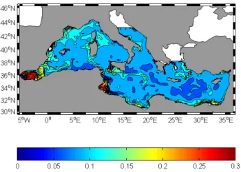
Fig. 4. Average surface phytoplankton concentrations (µmol N
dm−3)after 60 days.
Fig. 5. Average surface phytoplankton concentrations (µmol N
dm−3)after 120 days.
In the Aegean Sea, a full box including the Cretan Sea more northerly than 38◦N is considered starting from mea-sured profiles (McGill, 1970). In this marginal area it is con-venient to take into account the fluxes through the Aegean, in view of studies about climatic changes in the pelagic south-ern and deeper area. This second marginal region begins at 22◦E and ends at 28◦E, from 38◦N. Aegean nitrate vertical profile at 38◦N is reported in Fig. 3.
Potential temperature and salinity are restored to climato-logical values only in two areas: west of Gibraltar (6◦W) and in the model cells at 43◦N in the Adriatic Sea.
All over the basin, detritus is set to the 0.5 µmol N dm−3 initial condition from surface to 100 m depth; the value is null beneath. This accords with Coste et al. (1988) particulate matter, as measured in the inflowing Atlantic water.
Atmospheric loads and terrestrial inputs, as external inor-ganic nitrogen sources, are set to zero at this implementation phase of the system.
The following sequence shows the evolution of the phyto-plankton at surface. In the middle of the dynamical adjust-ment stage, see the 30 October snapshot, Fig. 4, the phyto-plankton generally increases in the 20 m upper layer. Start-ing from the initial homogeneous value of 0.0144 µmol N dm−3, biomass in terms of nitrogen reaches its highest con-centration values in the Alboran Sea, in the Gulf of Lions, in Sardinia and Sicily upwelling areas, in the Sirte Gulf and along Egyptian coast. A general increase of P is obtained.
Inorganic nitrogen at the same layer (not shown) is gener-ally depleted toward values of about 0.05 µmol N dm−3, pre-senting clear negative anomalies with respect to the starting value 0.0845. In the Gulf of Lions and in the other eutrophic areas high values of nutrient and of biomass coexist. A late summer evolution is evidently in progress, starting from ho-mogenous values toward zonal nutrient gradients, decreasing from west to east.
In Fig. 5 the surface phytoplankton concentration is shown after 120 days, on 29 December. An increase of biomass is evident in this pre-bloom period in a vast area of the western basin. The biomass maxima reach values about 0.2 µmol N dm−3, more than ten times the initial concentration of
sum-mer.
After 120 days, inorganic nitrogen, not shown, is anal-ogously at high values corresponding to the maxima in biomass at Fig. 5. The nutrient-rich sites are the Alboran Sea, Ligurian-Provenc¸al and Tyrrhenian Seas, large parts of Adriatic and Aegean, coastal areas along the African coast in the eastern basin.
The surface velocities at 20 m, not shown, show weaken-ing of the anticyclonic characteristics of the late summer sit-uation toward the winter one (Alboran Sea, southern Ionian, far Eastern Mediterranean). The along-shore currents inten-sify in these two months in the Gulf of Lions and Tyrrhenian coast; in the same late summer period, cyclonic gyres de-velop or intensify.
4 Twin experiment results and discussion
The evolution of the phytoplankton is shown in Fig. 6a. The three basin averages of the control run, of the free run, of the assimilated run are followed during the sixty-nine days of the evolution.
In the CR, total phytoplankton increases till its natural un-forced winter bloom. The FR evolves in a different way: starting from low biomass conditions, due to the summer biomass conditions prescribed at the beginning of the run, it shows a quick rise toward higher values, but of the same order, than the CR ones. The rise in the AR, more quick, shows tilt changes every seven days, caused by the assim-ilation, and reaches a bloom with lower values, but with a more damped overshoot than in the FR case, that is a re-sponse more close to the “sea-truth” CR in terms of biomass.
Fig. 6. Basin average phytoplankton (a) and zooplankton (b) evolutions along the 69 days of the CR, FR and AR in 1012g N (Tg N).
Fig. 7. Basin average inorganic nitrogen (a), detritus (b) and total nitrogen (c) evolutions along the 69 days of the CR, FR, AR in 1012g N (Tg N).
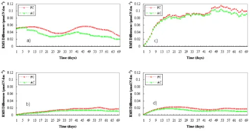
Fig. 8. Free–control run (squares) and assimilated–control run (triangles) root mean squared differences. The four plots show the rms
differences (µmol N dm−3)all over the basin for the phytoplankton (a), zooplankton (b), inorganic nitrogen (c) and detritus (d).
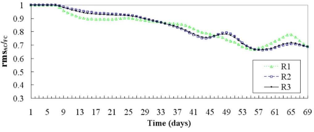
Fig. 9. Phytoplankton relative errors in R1 (0–20 m), R2 (20 m–bottom) and R3 (0 m–bottom).
This situation confirms the advantages gained by employing the assimilation procedure.
AR zooplankton behaviour (Fig. 6b) is very close to the control one and it begins to grow after the fourth assimila-tion cycle. This is due to higher grazing, determined by the increased phytoplankton present after assimilation. At the end of the simulation both experiments remain well beneath CR.
Inorganic nitrogen, detritus and total nitrogen (sum of the four compartments) are shown in Fig. 7. CR values are lower at the beginning in the inorganic nitrogen plate (Fig. 7a) be-cause there is a strong beginning uptake in the control run, with respect to the free and assimilation ones, for the dif-ferent biomass initial conditions. After 30 days inorganic nitrogen becomes greater in the control run, for the sum of two effects: the higher uptake experienced in the other two runs and the missing part of the initial biomass that still in-fluences.
As the last compartment, the detritus shows very low val-ues in FR and AR during the first part of the simulations, due
to the relatively low biomass values, and it cannot reach the high CR response (Fig. 7b) at the end of the simulation.
Total nitrogen (Fig. 7c) shows at the beginning a negative step because of the less biomass prescribed in FR and AR as initial conditions of the simulation. In the assimilation run recovery of nearer values to “sea-truth” total nitrogen is partially attained, but with no trend toward convergence. Related conclusion is that one winter mixing season is not sufficient for recovering total nitrogen bulk content.
According with Raicich and Rampazzo (2003), it is possi-ble to evaluate in a twin experiment the performance of the assimilation filter with respect to the free run by means of relative errors. Considering the assimilated, the free and the control biochemical tracer data, the expressions for the root mean squared differences are:
rmsAC = v u u u u t P i (Ai−Ci)2Voli P i Voli
Fig. 10. Zooplankton relative errors in R1, R2, and R3.
Fig. 11. Inorganic nitrogen relative errors in R1, R2 and R3.
rmsF C= v u u u u t P i (Fi−Ci)2Voli P i Voli
and the relative error is defined as: rmsAC/F C=
rmsAC rmsF C
in which i are the grid points (363 in longitude, 113 in lati-tude, 31 in depth); Ai, Fi, Ci are the biochemical tracer con-centrations at each grid point, respectively, of the assimilated, free and control run; Voli is the volume of the cell i.
For giving an insight in the different behaviour of the free and the assimilated evolutions, the root mean squared dif-ferences of the four variables, in sequence P, Z, N, D, are presented in Fig. 8. Both the root mean squared differences of the free run (rmsF Cin squares) and those of the assimila-tion run (rmsAC in triangles) with respect to the control run are shown for each ecosystem variable. The calculations are performed at a basin scale.
The phytoplankton rmsF Cstarts from an initial value, due to the decrease of the initial conditions of the phytoplank-ton, i.e. low summer values for the free run at the place of high winter control values. This evolution exhibits some
variability of the rms differences between the two runs, but very small values are never obtained. The relaxation to the “sea-truth” is not attained simply by dynamics and the root mean squared differences remain of the same order than the initial value, due to the local differences between the two runs. On the other hand, the phytoplankton rmsACstart from the same initial value and are pushed toward lower values by the assimilation procedure (Fig. 8a). The relative decrease is the indicator of the performance of the SOFA scheme and is given as relative error, rmsAC/F C, in the following, see Fig. 9. Also in this assimilated case, as in the free run, the root mean squared differences reach lower values at the end of the simulation; in any case, the integrated system performs better than the free one.
Zooplankton and detritus rmsAC are significantly lower than rmsF C (Figs. 8b and d). Improvements by means of the assimilation scheme are evident, but convergence toward the null initial values is not obtained in both cases.
Inorganic nitrogen rmsF Cstarts as well from null values, because N initial conditions are not changed; they become higher during the simulation and reach at the end nearly flat values about double than phytoplankton ones (Fig. 8c). This means that the phytoplankton is an important but not the dominant source of error in the system for this twin
Fig. 12. Detritus relative errors in R1, R2 and R3.
Fig. 13. Total nitrogen relative errors in R1, R2 and R3.
experiment. There is also an important part originated from N dynamics, and also Z and P can be relatively important. Also in the inorganic nitrogen case the assimilation shows some improvements.
The rmsAC/F C expressions are calculated at each of the sixty-nine days of the evolution discriminating three cases, respectively where data are assimilated, not assimilated, and all over the basin: the first range (R1) spans from surface to 20 m depth, the second one (R2) from 20 m to bottom, the third one (R3) from surface to bottom.
Figure 9 gives the evolution of the phytoplankton relative errors in R1, R2 and R3; the ordinates represent the assimi-lated run rms to the free one ratio, so that a good forecasting index lays below one. The better performance occurs in the R1 evolution. This is stepwise with oscillations around the 0.5 value, with approximately 50% better error at the end of the sixty-nine days. The trend of the phytoplankton in R2 is also good with final results of 0.6, with a result slightly worse than the all water column relative error.
Zooplankton relative errors (Fig. 10) remain the same in all the three chosen spatial partitions, approximately 0.7 at the end of the integration period. This value is also reached from inorganic nitrogen in the 0–20 m layer (Fig. 11); the minimum is reached because of the phytoplankton increase in the AR. Consequently a greater uptake is in effect, and the inorganic nitrogen reaches lower values than in the FR. The final effect is that the surface inorganic nitrogen is closer to the control run, with the relative improvement before day 35. R2 and R3 are practically not affected along all the inte-gration, reaching values around 0.95. Detritus (Fig. 12) has initially a behaviour lower in the R1 case with respect to the other two ranges, while at the end of the sixty-nine days all the three relative errors reach slightly higher values than 0.6. The total nitrogen relative errors are shown in Fig. 13, in-dicating striking differences among the deeper layers and the upper 20 m, where the biomass assimilation is performed. In the R2 and R3 rmsAC/F C, the values are very close to one with small oscillations when phytoplankton is assimilated
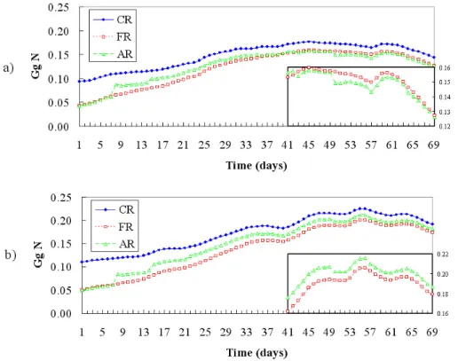
Fig. 14. Upper layer (0–20 m) Mediterranean total nitrogen content in 109 g N (Gg N) for CR, FR and AR. The contents are enlarged in the bottom right box after 41 days of the twin experiments.
Fig. 15. R1 (0–20 m) total nitrogen content in the western (a) and eastern basins (b) expressed in 109g N (Gg N) for CR, FR and AR. The contents are enlarged in the bottom right boxes after 41 days of the twin experiments.
and with a recovery of the free situation after each assim-ilation cycle. In the upper layer the relative errors de-crease at the beginning, but, after four weeks, R1 exhibits in-creased relative errors and after six assimilation cycles they become greater than one. Thus forecasting deteriorates at last, i.e. rmsAC become greater than rmsF C.
This anomaly is not evident at an overall basin scale. The R1 total nitrogen of the assimilated run (Fig. 14; see also the enlarged box) is always between the control and the free
run, indicating that, on a basin average, the result obtained through assimilation is nearer to the “sea-truth” than the free one. This suggests focussing to local effects for understand-ing what is happenunderstand-ing in the layer where the biomass is as-similated.
A different behaviour emerges discussing the R1 average total nitrogen contents in the western basin (Fig. 15a) and in the eastern one (Fig. 15b). The former is the signature in con-centration of the local deteriorating effects of the assimilation
Fig. 16. R1 (0–20 m) total nitrogen relative errors in the western (a) and eastern basins (b) .
univariate scheme. There are evident improvements of the total contents after the first three assimilation cycles in both cases; on the other hand, the FR total nitrogen reaches and overcomes that in the AR only in the western basin, see also the bottom right box in Fig. 15a during the last month of the simulation, but it remains well below in the eastern basin, Fig. 15b inner box. Both twin numerical experiments never reach in this surface layer the higher CR total nitrogen con-tents.
Figure 16 analyses the total nitrogen relative errors in the R1, upper western (Fig. 16a) and eastern (Fig. 16b) layers. All Mediterranean statistics, as given previously in Fig. 13 (R1), shows that this error becomes greater than one, indicat-ing deterioratindicat-ing forecastindicat-ing skill of the assimilation scheme. In the western basin evaluations, it is worth noting the pres-ence of these greater than one anomalies after the fifth assim-ilation cycle (Fig. 16a).
On the other hand, the eastern basin (Fig. 16b) shows, even in presence of an increased relative error after the fifth assim-ilation cycle, no deterioration of the forecasting, but only a relative worsening with respect to the first assimilation cy-cles.
Considering the upper layer evolution of the other vari-ables (not shown), the western basin is depicted as an in-termediate complexity ecosystem. It contains high phyto-plankton biomass with an important, four times less in nitro-gen units than that, influence of the zooplankton. Therefore
this regime produces high detritus export due to the sloppy feeding, which has time constant about one day, and due to the zooplankton specific mortality, with a five days rate. The eastern basin can instead be defined as an oligotrophic ecosystem, with scarce energy in the higher trophic levels. In fact, zooplankton is, in the twin experiments, about fifteen times less than phytoplankton biomass. Thus less production of sinking detritus is here present, in any case with a genera-tion time of about twenty days, the phytoplankton mortality rate.
5 Conclusions
A three-dimensional coupled physical-biochemical model of the Mediterranean Sea, consisting in GCM evolution of the winter bloom ecosystem variability, has been used in identi-cal twin experiments for testing a generic reduced-order opti-mal interpolation data assimilation method. Surface biomass data have been assimilated through SOFA at two quotas, 5 m and 15 m, as constraints of the trophic cycle freely simulated by NPZD description.
The results of this preliminary feasibility study show ad-vantages and limits of the chosen univariate methodology. The advantages are: efficiency of the reduced-order optimal interpolation in reducing the relative error of the phytoplank-ton, which is assimilated once at the end of each week; ability
of the ecosystem model in spreading the assimilated infor-mation from phytoplankton variable to the other biochemical ones.
Speaking in detail, the surface biomass constraints suc-cessfully drive phytoplankton concentrations toward better overall performance. Surface biomass takes about one month to reach season correct values, starting from summer initial conditions. There is a strong influence on phytoplankton er-ror decrease not only in the top 20 m, where biomass is as-similated, but also in the deeper layers. The relative error, assimilated run versus free run, is about 0.6.
The limits of the methodology consist in: inorganic nitro-gen error reduced mainly at surface by the surface biomass assimilation and poorly at an overall scale; slight corrections of the basin total nitrogen; small scale anomalies in the west-ern basin, where the assimilation scheme is nonperformant for the surface total nitrogen.
Even if root mean squared differences are generally smaller in the assimilation run than in the free run, for all the four biochemical variables, inorganic nitrogen exhibits a clear improvement only at surface, while in the interior the relative error remains about 0.95. The total nitrogen represents the weak point of this univariate methodology. The basin average shows poor convergence toward the richer “sea-truth” state of the ecosystem. Some limited recovery is attained only after the initial assimilation cycles. The conse-quence is that in this framework one winter assimilation stage cannot recover the deeper layer total nitrogen concentrations. For what regard the anomalies, the surface total nitrogen shows root mean squared differences higher in the assimi-lated run than in the free one. Such behaviour is shown as due to the Western Mediterranean trophic cycle, exporting more detritus from the surface layers. The regional analysis suggests that the present univariate approach aids in improv-ing total nitrogen forecastimprov-ing in oligotrophic ecosystems, like the Eastern Mediterranean. In presence of more complex interactions with the higher trophic levels, other assimila-tion strategies, possibly multivariate methodologies, should be proposed and verified in realistic basin scale experiments.
Acknowledgements. This work has been supported by
Mediter-ranean Forecasting System: Toward Environmental Predictions, E. C. Project EVH3-CT-2002-00075.
We wish to thank F. Raicich for his aid at the setup stage of this work, G. Padoan, for support as computer manager of the ORIGIN 300 at OGS, and C. Calonaci and G. Ballabio, system managers of the SP4 facilities at the Consorzio Interuniversitario del Nord-Est Italiano per il Calcolo Automatico-CINECA.
Edited by: N. Pinardi
References
Berland, B. R., Benzhitski, A. G., Burlakova, Z. P., Georgieva, L. V., Izmestieva, M. A., Kholodov, V. I., and Maestrini, S. Y.: Con-ditions hydrologiques estivales en M´editerran´ee, repartition du phytoplancton et de la mati`ere organique, Oceanol. Acta, 9(SP), 163–177, 1988.
Civitarese, G., Crise, A., Crispi, G., and Mosetti, R.: Circulation effects on nitrogen dynamics in the Ionian Sea, Oceanol. Acta, 19(6), 609–621, 1996.
Coste, B., Le Corre, P., and Minas, H. J.: Re-evaluation of the nu-trient exchanges in the Strait of Gibraltar, Deep-Sea Res., 35, 767–775, 1988.
De May, P. and Benkiran, M.: A Multivariate Reduced-order Op-timal Interpolation Method and its Application to the Mediter-ranean Basin-scale Circulation, in: Ocean Forecasting: concep-tual basis and applications, edited by: Pinardi, N. and Woods, J., Springer Verlag, 281–306, 2002.
Demirov, E. and Pinardi, N.: Simulation of the Mediterranean Sea circulation from 1979 to 1993: Part I. The interannual variability, J. Mar. Syst., 33-34, 23–50, 2002.
Eppley, R. W.: Temperature and phytoplankton growth in the sea, Fish. Bull., 70, 1063–1085, 1972.
Gordon, H. R. and Morel, A. Y.: Remote Assessment of Ocean Color for Interpretation of Satellite Visible Imagery. A review, Springer-Verlag, New York, pp. 114, 1983.
Manca, B., Burca, M., Giorgetti, A., Coatanoan, C., Garcia, M.-J., and Iona, A.: Physical and biochemical averaged vertical pro-files in the Mediterranean regions: an important tool to trace the climatology of water masses and to validate incoming data from operational oceanography, J. Mar. Syst., 48(1-4), 83–116, 2004. McGill, D. A.: Mediterranean Sea Atlas – distribution of
nutri-ent chemical properties, Woods Hole Oceanographic Institution, Woodshole, MA, 1970.
Monaco, A. and Peruzzi, S.: The Mediterranean Targeted Project MATER – a multiscale approach of the variability of a marine system – overview, J. Mar. Syst., 33-34, 3–21, 2002.
Osborne, J., Swift, J., and Flinchem, E. P.: OceanAtlas for MacIntosh©. National Science Foundation, 1992.
Pinardi, N., Baretta, J. W., Bianchi, M., Cr´epon, M., Crise, A., Rassoulzadegan, F., Thingstad, F., and Zavatarelli, M.: Coupled physical-biogeochemical models, in: Interdisciplinary research in the Mediterranean Sea, edited by: Lipiatou, E., EUR 17787, 316–342, 1997.
Raicich, F. and Rampazzo, A.: Observing System Simulation Ex-periments for the assessment of temperature sampling strategies in the Mediterranean Sea, Ann. Geoph., 21, 151–165, 2003. Raicich, F.: The assessment of temperature and salinity sampling
strategies in the Mediterranean Sea: idealized and real cases, Ocean Science, 2, 97–112, 2006.
Redfield, A. C., Ketchum, B. H., and Richards, F. A.: The influ-ence of Sea Water, in: The Sea, vol. 2, edited by: Hill, M. N., Interscience, New York, 26–77, 1963.
Sverdrup, H. U., Johnson, M. W., and Fleming, R. H.: The Oceans: their Physics, Chemistry and General Biology, Prentice Hall New York, pp. 1087, 1942.
Triantafyllou, G., Hoteit, I., Korres, G., and Petihakis, G.: Ecosystem Modelling and Data Assimilation of Physical-Biogeochemical processes in Shelf and Regional Areas of the Mediterranean Sea, Appl. Num. Anal. Comp. Math., 2(2), 262–
280, 2005.
Vecchi, G. A. and Harrison, M. J.: An observing system simulation experiment for the Indian Ocean, J. Climate, in press, 2006.
Zavatarelli, M., Raicich, F., Bregant, D., Russo, A., and Artegiani, A.: Climatological characteristics of the Adriatic Sea, J. Mar. Syst., 18(1–3), 227–263, 1998.