HAL Id: hal-00927047
https://hal.archives-ouvertes.fr/hal-00927047
Submitted on 10 Jan 2014
HAL is a multi-disciplinary open access
archive for the deposit and dissemination of
sci-entific research documents, whether they are
pub-lished or not. The documents may come from
teaching and research institutions in France or
abroad, or from public or private research centers.
L’archive ouverte pluridisciplinaire HAL, est
destinée au dépôt et à la diffusion de documents
scientifiques de niveau recherche, publiés ou non,
émanant des établissements d’enseignement et de
recherche français ou étrangers, des laboratoires
publics ou privés.
Sparsity and the Bayesian Perspective
Jean-Luc Starck, David Donoho, Jalal M. Fadili, Anais Rassat
To cite this version:
Jean-Luc Starck, David Donoho, Jalal M. Fadili, Anais Rassat. Sparsity and the Bayesian
Perspec-tive. Astronomy and Astrophysics - A&A, EDP Sciences, 2013, 552, A133, 5 pp.
�10.1051/0004-6361/201321257�. �hal-00927047�
DOI:10.1051/0004-6361/201321257
c
�ESO 2013
&
Astrophysics
Sparsity and the Bayesian perspective
J.-L. Starck
1, D. L. Donoho
2, M. J. Fadili
3, and A. Rassat
3,1,41 Laboratoire AIM, UMR CEA-CNRS-Paris 7, Irfu, Service d’Astrophysique, CEA Saclay, 91191 Gif-sur-Yvette Cedex, France
e-mail: [email protected]
2 Department of Statistics, Stanford University, Stanford CA, 94305, USA
3 GREYC CNRS-ENSICAEN-Université de Caen, 6 Bd du Maréchal Juin, 14050 Caen Cedex, France
4 Laboratoire d’Astrophysique, École Polytechnique Fédérale de Lausanne (EPFL), Observatoire de Sauverny, 1290 Versoix,
Switzerland
Received 7 February 2013 / Accepted 15 February 2013
ABSTRACT
Sparsity has recently been introduced in cosmology for weak-lensing and cosmic microwave background (CMB) data analysis for different applications such as denoising, component separation, or inpainting (i.e., filling the missing data or the mask). Although it gives very nice numerical results, CMB sparse inpainting has been severely criticized by top researchers in cosmology using arguments derived from a Bayesian perspective. In an attempt to understand their point of view, we realize that interpreting a regularization penalty term as a prior in a Bayesian framework can lead to erroneous conclusions. This paper is by no means against the Bayesian approach, which has proven to be very useful for many applications, but warns against a Bayesian-only interpretation in data analysis, which can be misleading in some cases.
Key words.methods: statistical – cosmic background radiation – methods: data analysis
1. Introduction
Bayesian methodology is extremely popular in cosmology. It proposes a very elegant framework for dealing with uncertain-ties and for using our knowledge under the form of priors in order to solve a given inverse problem (Hobson et al. 2010;
Mielczarek et al. 2009). The huge success of Bayesian meth-ods in cosmology is well illustrated inTrotta(2008) with a fig-ure on the number of papers with the word “Bayesian” in the title as a function of the publication year. Bayesian techniques have been used for many applications such as model selection (Kilbinger et al. 2010; Trotta 2012), primordial power spec-trum analysis (Kawasaki & Sekiguchi 2010), galactic surveys design (Watkinson et al. 2012), or cosmological parameters es-timations (March et al. 2011). Bayesian methods are now com-monly used at almost every step in the cosmic microwave back-ground (CMB) pipeline experiments, for point source removal (Argüeso et al. 2011; Carvalho et al. 2012), noise level esti-mation (Wehus et al. 2012), component separation (Dickinson et al. 2009), cosmological parameter estimation (Efstathiou et al. 2010), non-Gaussianity studies (Elsner & Wandelt 2010;Feeney et al. 2012), or inpainting (Bucher & Louis 2012; Kim et al. 2012).
Sparsity has recently been proposed for CMB data analy-sis for component separation (Bobin et al. 2013) and inpaint-ing (Abrial et al. 2007; Abrial et al. 2008;Starck et al. 2013). The sparsity-based inpainting approach has been successfully used for two different CMB studies, the CMB weak-lensing on Planck simulated data (Perotto et al. 2010;Plaszczynski et al. 2012), and the analysis of the integrated Sachs-Wolfe effect (ISW) on WMAP data (Dupé et al. 2011; Rassat et al. 2012). In both cases, the authors showed using Monte-Carlo simula-tions that the statistics derived from the inpainted maps can be
trusted at a high confidence level, and that sparsity-based in-painting can indeed provide an easy and effective solution to the problem of large Galactic mask. However, even if these simula-tions have shown that sparsity-based inpainting does not destroy CMB weak-lensing, ISW signals, or large-scale anomalies in the CMB, the CMB community is very reluctant to use this concept. This has lead to very animated discussions in conferences. During these discussions it has come up that cosmologists of-ten resort to a Bayesian interpretation of sparsity. Hence, they summarize the sparse regularization to the maximum a posteri-ori (MAP) estimator assuming the solution follows a Laplacian distribution. From this perspective, several strong arguments against the use of sparsity for CMB analysis were raised:
1. Sparsity consists in assuming an anisotropic and a non-Gaussian prior, which is unsuitable for the CMB, which is Gaussian and isotropic.
2. Sparsity violates rotational invariance.
3. The �1 norm that is used for sparse inpainting arose purely out of expediency because under certain circumstances it re-produces the results of the �0pseudo-norm (which arises nat-urally in the context of strict, as opposed to weak, sparsity) without requiring combinatorial optimization.
4. There is no mathematical proof that sparse regularization preserves/recovers the original statistics.
The above arguments result from a Bayesian point of view of the sparsity concept. In this paper we explain in detail why the above arguments are not rigorously valid and why sparsity is not in contradiction with a Bayesian interpretation.
A&A 552, A133 (2013)
2. Sparse regularization of inverse problems
2.1. Inverse problem regularization
Many data processing problems can be formalized as a linear inverse problem,
y = Ax + ε, (1)
where y ∈ Fm is a vector of noisy measurements (real with F = R, or complex F = C), ε is an m-dimensional vector of additive noise, x is the perfect n-dimensional unobserved vector of interest, and A:Fn → Fm is a linear operator. For example, the inpainting problem corresponds to the case where we want to recover some missing data, in which case A is a binary matrix with fewer rows than columns (m < n), and contains only one value equal to 1 per row, with all other values equal to 0.
Finding x when the values of y and A are known is a linear inverse problem. When it does not have a unique and stable so-lution, it is ill-posed and a regularization is necessary to reduce the space of candidate solutions.
A very popular regularization in astronomy is the well-known Bayesian maximum entropy method (MEM), which is based on the principle that we want to select the simplest solu-tion which fits the data. Sparsity has recently emerged as very powerful approach for regularization (Starck et al. 2010). 2.2. Strict and weak sparsity
A signal x considered as a vector in Fn is said to be sparse if most of its entries are equal to zero. If k numbers of the n sam-ples are equal to zero, where k < n, then the signal is said to be k-sparse. Generally, signals are not sparse in direct space, but can be sparsified by transforming them to another domain. Think for instance of a purely sinusoidal signal which is 1-sparse in the Fourier domain, while it is clearly dense in the original one. In the so-called sparsity synthesis model, a signal can be repre-sented as the linear expansion
x= Φα = t �
i=1
φiαi, (2)
where α are the synthesis coefficients of x, Φ = (φ1, . . . , φt) is the dictionary whose columns are t elementary waveforms φi also called atoms. In the language of linear algebra, the dic-tionary Φ is a b × t matrix whose columns are the normalized atoms, supposed here to be normalized to a unit �2-norm, i.e., ∀i ∈[1, t], �φi�22=�nn=1|φi[n]|2=1.
A signal can be decomposed in many dictionaries, but the best one is the one with the sparsest (most economical) represen-tation of the signal. In practice, it is convenient to use dictionar-ies with fast implicit transforms (such as the Fourier transform, wavelet transforms, etc.) which allow us to directly obtain the coefficients and reconstruct the signal from these coefficients us-ing fast algorithms runnus-ing in linear or almost linear time (unlike matrix-vector multiplications). The Fourier, wavelet, and dis-crete cosine transforms are among the most popular dictionaries. Most natural signals however are not exactly sparse but rather concentrated near a small set. Such signals are termed compressibleor weakly sparse in the sense that the sorted mag-nitudes � � �α(i) � � �, i.e., � � �α(1) � � � > � � �α(2) � � � , ..., > � � �α(t) � � �, of the sequence of coefficients α decay quickly according to a power law, i.e., � � �α(i) � � � �Ci
−1/r,i = 1, . . . , t, where C is a constant. The larger r is, the faster the amplitudes of coefficients decay, and the more
compressible the signal is. In turn, the non-linear �2 approxima-tion error of α (and x) from its M largest entries in magnitude also decrease quickly. One can think, for instance, of the wavelet coefficients of a smooth signal away from isotropic singularities, or the curvelet coefficients of a piecewise regular image away from smooth contours. A comprehensive account on sparsity of signals and images can be found inStarck et al.(2010).
2.3. Sparse regularization for inverse problems In the following, for a vector z we denote �z�p
p = �i|zi|p for p ≥ 0. In particular, for p ≥ 1, this is the pth power of the �p norm, and for p = 0, we get the �0pseudo-norm which counts the number of non-zero entries in z. The �0regularized problem amounts to minimizing
˜α ∈ argmin
α �y − AΦα� 2
2+ λ�α�0, (3)
where λ is a regularization parameter. A solution ˜x is recon-structed as ˜x = Φ ˜α. Clearly, the goal of Eq. (3) is to minimize the number of non-zero coefficients describing the sought after signal while ensuring that the forward model is faithful to the observations.
Solving Eq. (3) is however known to be NP-hard. The �1 norm has been proposed as a tight convex relaxation of Eq. (3) leading to the minimization problem
˜α ∈ argmin α
�y − AΦα�22+ λ�α�1, (4)
where λ is again a regularization parameter different from that of Eq. (3). There has been a tremendous amount of work where re-searchers spanning a wide range of disciplines have studied the structural properties of minimizers of Eq. (4) and its equivalence with Eq. (3). Equation (4) is computationally appealing and can be efficiently solved, and it has also been proved that under ap-propriate circumstances, Eq. (4) produces exactly the same so-lutions as Eq. (3), see e.g.,Donoho(2006b) and the overview in the monograph (Starck et al. 2010).
3. Sparsity prior and Bayesian prior
3.1. Bayesian framework
In the Bayesian framework, a prior is imposed on the object of interest through a probability distribution. For instance, assume that coefficients α are i.i.d. Laplacian with the scale parameter τ, i.e., the density Pα(α) ∝ e−τ�α�1, and the noise ε is zero-mean white Gaussian with variance σ2, i.e., the conditional density PY|α(y) = (2πσ2)−m/2e−�y−AΦα�
2
2/(2σ2). By traditional Bayesian
arguments, the MAP estimator is obtained by maximizing the conditional posterior density Pα|Y(α) ∝ PY|α(y)Pα(α), or equiv-alently by minimizing its anti-log version
min α
1
2σ2�y − AΦα�22+ τ �α�1. (5)
This is exactly Eq. (4) by identifying λ = 2σ2τ. This resem-blance has led Bayesian cosmologists to raise the four criticisms mentioned in the introduction. But as we will discuss shortly, their central argument is not used in the right sense, which can yield misleading conclusions.
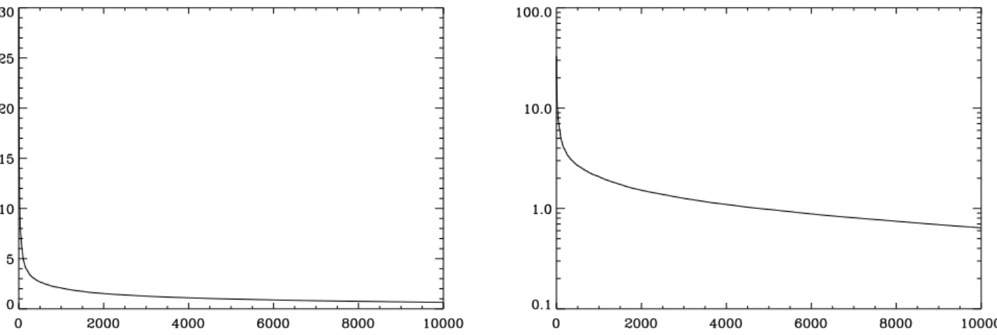
Fig. 1.Left: amplitude (absolute value) of the spherical harmonic coefficients versus their index, when the coefficients are sorted from the largest amplitude to the smallest. Right: same plot with the y-axis in log.
3.2. Should �1regularization be the MAP?
In Bayesian cosmology, the following shortcut is often made: if a prior is at the basis of an algorithm, then to use this algo-rithm, the resulting coefficients must be distributed according to this prior. But it is a false logical chain in general, and high-dimensional phenomena completely invalidate it.
For instance, Bayesian cosmologists claim that �1 regular-ization is equivalent to assuming that the solution is Laplacian and not Gaussian, which would be unsuitable for the case of CMB analysis. This argument however assumes that a MAP es-timate follows the distribution of the prior. But it is now well-established that MAP solutions substantially deviate from the prior model, and that the disparity between the prior and the ef-fective distribution obtained from the true MAP estimate is a permanent contradiction in Bayesian MAP estimation (Nikolova 2007). Even the supposedly correct �2prior would yield an esti-mate (Wiener, which coincides with the MAP and posterior con-ditional mean) whose covariance is not that of the prior.
In addition, rigorously speaking, this MAP interpretation of �1 regularization is not the only possible interpretation. More precisely, it was shown inGribonval et al.(2011a) andBaraniuk et al. (2010) that solving a penalized least squares regression problem with penalty ψ(α) (e.g. the �1norm) should not neces-sarily be interpreted as assuming a Gibbsian prior C exp(−ψ(α)) and using the MAP estimator. In particular, for any prior Pα, the conditional mean can also be interpreted as a MAP with some prior C exp(−ψ(α)). Conversely, for certain penalties ψ(α), the solution of the penalized least squares problem is indeed the conditional posterior mean, with a certain prior Pα(α) which is generally different from C exp(−ψ(α)).
In summary, the MAP interpretation of such penalized least-squares regression can be misleading, and using a MAP estima-tion, the solution does not necessarily follow the prior distribu-tion, and an incorrect prior does not necessarily lead to a wrong solution. What we are claiming here are facts that were stated and proved as rigorous theorems in the literature.
3.3. Compressed sensing: the Bayesian interpretation inadequacy
A beautiful example to illustrate this is the compressed sens-ing scenario (Donoho 2006a;Candès & Tao 2006), which tells us that a k-sparse, or compressible n-dimensional signal x can be recovered either exactly, or to a good approximation, from
much less random measurements m than the ambient dimen-sion n, if m is sufficiently larger than the intrinsic dimendimen-sion of x. Clearly, the underdetermined linear problem, y = Ax, where A is drawn from an appropriate random ensemble, with fewer equa-tions than unknown, can be solved exactly or approximately, if the underlying object x is sparse or compressible. This can be achieved by solving a computationally tractable �1-regularized convex optimization program.
If the underlying signal is exactly sparse, in a Bayesian framework, this would be a completely absurd way to solve the problem, since the Laplacian prior is very different from the ac-tual properties of the original signal (i.e., k coefficients different from zero). In particular, what compressed sensing shows is that we can have prior A be completely true, but utterly impossible to use for computation time or any other reason, and we can use prior B instead and get the correct results. Therefore, from a Bayesian point of view, it is rather difficult to understand not only that the �1 norm is adequate, but also that it leads to the exact solution.
3.4. The prior misunderstanding
Considering the chosen dictionary Φ as the spherical harmonic transform, the coefficients α are now α = �al,m�l=0,...,lmax,m=−l,...,l. The standard CMB theory assumes that the values of al,m are the realizations of a collection of heteroscedastic complex zero-mean Gaussian random variables with variances Cl/2, where Cl is the true power spectrum. Using a �1 norm is then interpreted in the Bayesian framework as having a Laplacian prior on each al,mwhich contradicts the underlying CMB theory. However, as argued above, from the regularization point of view, the �1norm merely promotes a solution x such that its spherical harmonic coefficients are (nearly) sparse. There is no assumption at all on the properties related to a specific al,m. In fact, there is no ran-domness here and the al,m values do not even have to be inter-preted as a realization of a random variable. Therefore, whatever the underlying distribution for a given al,m(if its exists), it need not be interpreted as Laplacian under the �1regularization. The CMB can be Gaussian or not, isotropic or not, and there will be no contradiction with the principle of using the �1norm to solve the reconstruction problem (e.g., inpainting). What is important is that the sorted absolute values of the CMB spherical harmon-ics coefficients presents a fast decay. This is easily verified using a CMB map, data, or simulation. This is well illustrated by Fig.1
A&A 552, A133 (2013) which shows this decay for the nine-year WMAP data set. As we
can see, the compressibility assumption is completely valid.
4. Discussion of the Bayesian criticisms
• Sparsity consists in assuming an anisotropy and a non-Gaussian prior, which is unsuitable for the CMB, which is Gaussian and isotropic.We have explained in the previous section that this MAP interpretation of �1 regularization is misleading, and also that there is no assumption at all on the underlying stochastic process. The CMB sparsity-based recovery is a purely data-driven regularization approach; the sorted absolute values of the spherical harmonic coefficients presents a fast decay, as seen on real data or simulations, and this motivates the sparse regularizations.
There is no assumption that the CMB is Gaussian or isotropic, but there is also no assumption that it is non-Gaussian or anisotropic. In this sense, using the �1-regularized inpainting to test if the CMB is indeed Gaussian and isotropic may be better than other methods, in-cluding Wiener filtering, which in the Bayesian framework assumes Gaussianity and isotropy. Furthermore, the Wiener estimator will also require knowing the underlying power spectrum (i.e., the theoretical Cl) which is an even stronger prior.
• Sparsity violates rotational invariance.The criticicism here is that linear combinations of independent exponentials are not independent exponentials; therefore, isotropy is neces-sarily violated, unless the alm are Gaussian. But again, our arguments for �1 regularization are borrowed from approxi-mation theory and harmonic analysis, and this does not con-tradict the idea that the alm coefficients can be realizations of a sequence of heteroscedastic Gaussian variables. The �1 norm regularization will be adequate if the sorted coefficients amplitudes follow a fast decay, which is always verified with CMB data. Indeed, as we already mentioned, a set of pa-rameters xi, where each xi is a realization of a Gaussian process of mean 0 and variance Vi, can present a fast de-cay when we plot the sorted absolute values of xi. In the case of CMB spherical harmonic coefficients verifying this is straightforward.
• The �1 norm that is used for sparse inpainting arose purely out of expediency because under certain circumstances it re-produces the results of the �0pseudo-norm.First, we would like to correct a possible misunderstanding: �1 regulariza-tion can provably recover both strictly and weakly sparse signals, while being stable to noise. In the strictly sparse case, �1 norm minimization can recover the right solution although the prior is not correct from a Bayesian point of view. In the compressible case, the recovery is up to a good approximation, as good as an oracle that would give the best M-term approximation of the unknown signal (i.e., �0-solution). What is criticized as an “expedient” prior is ba-sically at the heart of regularization theory, for instance here �1provides strong theoretical recovery guarantees under ap-propriate conditions. A closer look at the literature of inverse problems shows that these guarantees are possible beyond the compressed sensing scenario.
• There is no mathematical proof that sparse regularization preserves/recovers the original statistics.This is true, but this argument is not specific to �1 regularized inpainting. Even worse, as detailed and argued in the previous section, the posterior distribution generally deviates from the prior, and even if one uses the MAP with the correct Gaussian prior,
the MAP estimate (Wiener) will not have the covariance of the prior.
Another point to mention is that the CMB is never a pure Gaussian random field, even if the standard ΛCDM cosmo-logical model is truly valid. We know that the CMB is at least contaminated by non-Gaussian secondary anisotropies such as weak-lensing or kinetic Sunyaev-Zel’dovich (SZ) effects. Therefore the original CMB statistics are likely to be better preserved by an inpainting method that does not assume Gaussianity (but nonetheless allows it), rather than by a method which has an explicit Gaussian assumption. Moreover, if the CMB is not Gaussian, then one can clearly anticipate that the Wiener estimate does not preserve the original statistics.
Finally, it appears unfair to criticize sparsity-regularised in-verse problems on the mathematical side. A quick look at the literature shows the vitality of the mathematics community, both pure and applied, and the large amount of theoretical guarantees (deterministic and frequentist statistical settings) that have been devoted to �1regularization. In particular, the-oretical guarantees of �1-based inpainting can be found in King et al.(2013) on the Cartesian grid, and of sparse recov-ery on the sphere inRauhut & Ward(2012).
5. Conclusions
We have shown that Bayesian cosmologists’ criticisms about sparse inpainting are based on a false logical chain, which con-sists in assuming that if a prior is at the basis of an algorithm, then to use this algorithm, the resulting coefficients must be dis-tributed according to this prior. Compressed sensing theory is a nice counter-example, where it is mathematically proved that other prior, than the true one can lead, under some conditions, to the correct solution. Therefore, we cannot understand how a regularization penalty has an impact on a solution of an inverse problem just by expressing the prior which derives this penalty. To understand this we also need to take into account the operator involved in the inverse problem, and this requires much deeper mathematical developments than a simple Bayesian interpreta-tion. Compressed sensing theory shows that for some operators, beautiful geometrical phenomena allow us to recover perfectly the solution of an underdetermined inverse problem. Similar re-sults were derived for a random sampling on the sphere (Rauhut & Ward 2012).
We do not claim in this paper that sparse inpainting is the best solution for inpainting, but we have showed that the ar-guments raised against it are incorrect, and that if Bayesian methodology offers a very elegant framework that is extremely useful for many applications, we should be careful not to be monolithic in the way we address a problem. In practice, it may be useful to use several inpainting methods to better understand the CMB statistics, and it is clear that sparsity based inpainting does not require making any assumptions about the Gaussianity nor about the isotropy, nor does it need to have a theoretical C� as an input.
Acknowledgements. The authors thank Benjamin Wandelt, Mike Hobson, Jason McEwen, Domenico Marinucci, Hiranya Peiris, Roberto Trotta, and Tom Loredo for the useful and animated discussions. This work was supported by the French National Agency for Research (ANR -08-EMER-009-01), the European Research Council grant SparseAstro (ERC-228261), and the Swiss National Science Foundation (SNSF).
References
Abrial, P., Moudden, Y., Starck, J., et al. 2007, J. Fourier Anal. Appl., 13, 729 Abrial, P., Moudden, Y., Starck, J., et al. 2008, Statist. Methodol., 5, 289 Argüeso, F., Salerno, E., Herranz, D., et al. 2011, MNRAS, 414, 410 Baraniuk, R., Cevher, V., & Wakin, M. 2010, Proc. IEEE, 98, 959 Bobin, J., Starck, J.-L., Sureau, F., & Basak, S. 2013, A&A, 550, A73 Bucher, M., & Louis, T. 2012, MNRAS, 424, 1694
Candès, E., & Tao, T. 2006, IEEE Trans. Info. Theory, 52, 5406
Carvalho, P., Rocha, G., Hobson, M. P., & Lasenby, A. 2012, MNRAS, 427, 1384
Dickinson, C., Eriksen, H. K., Banday, A. J., et al. 2009, ApJ, 705, 1607 Donoho, D. 2006a, IEEE Trans. Info. Theory, 52, 1289
Donoho, D. 2006b, Comm. Pure Appl. Math., 59, 907
Dupé, F.-X., Rassat, A., Starck, J.-L., & Fadili, M. J. 2011, A&A, 534, A51 Efstathiou, G., Ma, Y.-Z., & Hanson, D. 2010, MNRAS, 407, 2530 Elsner, F., & Wandelt, B. D. 2010, ApJ, 724, 1262
Feeney, S. M., Johnson, M. C., McEwen, J. D., Mortlock, D. J., & Peiris, H. V. 2012 [arXiv:1210.2725]
Gribonval, R., Cevher, V., & Davies, M. E. 2011 [arXiv:1102.1249]
Hobson, M. P., Jaffe, A. H., Liddle, A. R., Mukeherjee, P., & Parkinson, D. 2010, Bayesian Methods in Cosmology
Kawasaki, M., & Sekiguchi, T. 2010, J. Cosmol. Astropart. Phys., 2010, 013
Kilbinger, M., Wraith, D., Robert, C., et al. 2010, MNRAS, 405, 2381 Kim, J., Naselsky, P., & Mandolesi, N. 2012, ApJ, 750, L9
King, E. J., Kutyniok, G., & Zhuang, X. 2013, J. Math. Imaging Vision, submitted
March, M. C., Trotta, R., Berkes, P., Starkman, G. D., & Vaudrevange, P. M. 2011, MNRAS, 418, 2308
Mielczarek, J., Szydlowski, M., & Tambor, P. 2009 [arXiv:0901.4075] Nikolova, M. 2007, Inverse Problems and Imaging, 1, 399
Perotto, L., Bobin, J., Plaszczynski, S., Starck, J., & Lavabre, A. 2010, A&A, 519, A4
Plaszczynski, S., Lavabre, A., Perotto, L., & Starck, J.-L. 2012, A&A, 544, A27 Rassat, A., Starck, J.-L., & Dupe, F. X. 2012, A&A, submitted
Rauhut, H., & Ward, R. 2012, J. Approx. Theory, 164
Starck, J.-L., Murtagh, F., & Fadili, M. 2010, Sparse Image and Signal Processing (Cambridge University Press)
Starck, J.-L., Fadili, M. J., & Rassat, A. 2013, A&A, 550, A15 Trotta, R. 2008, Contemp. Phys., 49, 71
Trotta, R. 2012, in Astrostatistics and Data Mining, eds. L. M. Sarro, L. Eyer, W. O’Mullane, & J. De Ridder (New York: Springer), Springer Series in Astrostatistics, 2, 3
Watkinson, C., Liddle, A. R., Mukherjee, P., & Parkinson, D. 2012, MNRAS, 424, 313