HAL Id: cea-01135442
https://hal-cea.archives-ouvertes.fr/cea-01135442
Submitted on 25 Mar 2015
HAL is a multi-disciplinary open access
archive for the deposit and dissemination of
sci-entific research documents, whether they are
pub-lished or not. The documents may come from
teaching and research institutions in France or
abroad, or from public or private research centers.
L’archive ouverte pluridisciplinaire HAL, est
destinée au dépôt et à la diffusion de documents
scientifiques de niveau recherche, publiés ou non,
émanant des établissements d’enseignement et de
recherche français ou étrangers, des laboratoires
publics ou privés.
Astropy: A community Python package for astronomy
Thomas P. Robitaille, Erik J. Tollerud, Perry Greenfield, Michael
Droettboom, Erik Bray, Tom Aldcroft, Matt Davis, Adam Ginsburg, Adrian
M. Price-Whelan, Wolfgang E. Kerzendorf, et al.
To cite this version:
Thomas P. Robitaille, Erik J. Tollerud, Perry Greenfield, Michael Droettboom, Erik Bray, et al..
Astropy: A community Python package for astronomy. Astronomy and Astrophysics - A&A, EDP
Sciences, 2013, 558, pp.A33. �10.1051/0004-6361/201322068�. �cea-01135442�
DOI:10.1051/0004-6361/201322068 c
ESO 2013
Astrophysics
&
Astropy: A community Python package for astronomy
The Astropy Collaboration, Thomas P. Robitaille
1, Erik J. Tollerud
2,3, Perry Greenfield
4, Michael Droettboom
4,
Erik Bray
4, Tom Aldcroft
5, Matt Davis
4, Adam Ginsburg
6, Adrian M. Price-Whelan
7, Wolfgang E. Kerzendorf
8,
Alexander Conley
6, Neil Crighton
1, Kyle Barbary
9, Demitri Muna
10, Henry Ferguson
4, Frédéric Grollier
12,
Madhura M. Parikh
11, Prasanth H. Nair
12, Hans M. Günther
5, Christoph Deil
13, Julien Woillez
14, Simon Conseil
15,
Roban Kramer
16, James E. H. Turner
17, Leo Singer
18, Ryan Fox
12, Benjamin A. Weaver
19, Victor Zabalza
13,
Zachary I. Edwards
20, K. Azalee Bostroem
4, D. J. Burke
5, Andrew R. Casey
21, Steven M. Crawford
22,
Nadia Dencheva
4, Justin Ely
4, Tim Jenness
23,24, Kathleen Labrie
25, Pey Lian Lim
4, Francesco Pierfederici
4,
Andrew Pontzen
26,27, Andy Ptak
28, Brian Refsdal
5, Mathieu Servillat
29,5, and Ole Streicher
301 Max-Planck-Institut für Astronomie, Königstuhl 17, 69117 Heidelberg, Germany
e-mail: [email protected]
2 Department of Astronomy, Yale University, PO Box 208101, New Haven, CT 06510, USA 3 Hubble Fellow
4 Space Telescope Science Institute, 3700 San Martin Drive, Baltimore, MD 21218, USA 5 Harvard-Smithsonian Center for Astrophysics, 60 Garden Street, Cambridge, MA 02138, USA 6 Center for Astrophysics and Space Astronomy, University of Colorado, Boulder, CO 80309, USA 7 Department of Astronomy, Columbia University, Pupin Hall, 550W 120th St., New York, NY 10027, USA
8 Department of Astronomy and Astrophysics, University of Toronto, 50 Saint George Street, Toronto, ON M5S3H4, Canada 9 Argonne National Laboratory, High Energy Physics Division, 9700 South Cass Avenue, Argonne, IL 60439, USA
10 Department of Astronomy, Ohio State University, Columbus, OH 43210, USA 11 S.V.National Institute of Technology, 395007 Surat., India
12 Independent developer
13 Max-Planck-Institut für Kernphysik, PO Box 103980, 69029 Heidelberg, Germany
14 European Southern Observatory, Karl-Schwarzschild-Str. 2, 85748 Garching bei München, Germany
15 Laboratoire d’Astrophysique de Marseille, OAMP, Université Aix-Marseille et CNRS, 13388 Marseille, France 16 ETH Zürich, Institute for Astronomy, Wolfgang-Pauli-Strasse 27, Building HIT, Floor J, 8093 Zurich, Switzerland 17 Gemini Observatory, Casilla 603, La Serena, Chile
18 LIGO Laboratory, California Institute of Technology, 1200 E. California Blvd., Pasadena, CA 91125, USA 19 Center for Cosmology and Particle Physics, New York University, New York, NY 10003, USA
20 Department of Physics and Astronomy, Louisiana State University, Nicholson Hall, Baton Rouge, LA 70803, USA
21 Research School of Astronomy and Astrophysics, Australian National University, Mount Stromlo Observatory, via Cotter Road,
Weston Creek ACT 2611, Australia
22 SAAO, PO Box 9, Observatory 7935, 7925 Cape Town, South Africa 23 Joint Astronomy Centre, 660 N. A‘oh¯ok¯u Place, Hilo, HI 96720, USA 24 Department of Astronomy, Cornell University, Ithaca, NY 14853, USA 25 Gemini Observatory, 670 N. A‘oh¯ok¯u Place, Hilo, HI 96720, USA
26 Oxford Astrophysics, Denys Wilkinson Building, Keble Road, Oxford OX1 3RH, UK 27 Department of Physics and Astronomy, University College London, London WC1E 6BT, UK 28 NASA Goddard Space Flight Center, X-ray Astrophysics Lab Code 662, Greenbelt, MD 20771, USA 29 Laboratoire AIM, CEA Saclay, Bât. 709, 91191 Gif-sur-Yvette, France
30 Leibniz-Institut für Astrophysik Potsdam (AIP), An der Sternwarte 16, 14482 Potsdam, Germany
Received 12 June 2013/ Accepted 23 July 2013
ABSTRACT
We present the first public version (v0.2) of the open-source and community-developed Python package, Astropy. This package provides core astronomy-related functionality to the community, including support for domain-specific file formats such as flexible image transport system (FITS) files, Virtual Observatory (VO) tables, and common ASCII table formats, unit and physical quantity conversions, physical constants specific to astronomy, celestial coordinate and time transformations, world coordinate system (WCS) support, generalized containers for representing gridded as well as tabular data, and a framework for cosmological transformations and conversions. Significant functionality is under active development, such as a model fitting framework, VO client and server tools, and aperture and point spread function (PSF) photometry tools. The core development team is actively making additions and enhancements to the current code base, and we encourage anyone interested to participate in the development of future Astropy versions.
Key words.methods: data analysis – methods: miscellaneous – virtual observatory tools
A&A 558, A33 (2013) 1. Introduction
The Python programming language1 has become one of the fastest-growing programming languages in the astronomy com-munity in the last decade (see e.g.Greenfield 2011, for a recent review). While there have been a number of efforts to develop Python packages for astronomy-specific functionality, these ef-forts have been fragmented, and several dozens of packages have been developed across the community with little or no coordi-nation. This has led to duplication and a lack of homogeneity across packages, making it difficult for users to install all the required packages needed in an astronomer’s toolkit. Because a number of these packages depend on individual or small groups of developers, packages are sometimes no longer maintained, or simply become unavailable, which is detrimental to long-term research and reproducibility.
Motivated by these issues, the Astropy project was started in 2011 out of a desire to bring together developers across the field of astronomy in order to coordinate the development of a com-mon set of Python tools for astronomers and simplify the land-scape of available packages. The project has grown rapidly, and to date, over 200 individuals are signed up to the development mailing list for the Astropy project2.
One of the primary aims of the Astropy project is to develop a core astropy package that covers much of the astronomy-specific functionality needed by researchers, complementing more general scientific packages such as NumPy (Oliphant
2006;Van Der Walt et al. 2011) and SciPy (Jones et al. 2001),
which are invaluable for numerical array-based calculations and more general scientific algorithms (e.g. interpolation, integra-tion, clustering). In addiintegra-tion, the Astropy project includes work on more specialized Python packages (which we call affiliated packages) that are not included in the core package for various reasons: for some the functionality is in early stages of devel-opment and is not robust; the license is not compatible with Astropy; the package includes large files; or the functionality is mature, but too domain-specific to be included in the core package.
The driving interface design philosophy behind the core package is that code using astropy should result in concise and easily readable code, even by those new to Python. Typical op-erations should appear in code similar to how they would appear if expressed in spoken or written language. Such an interface results in code that is less likely to contain errors and is eas-ily understood, enabling astronomers to focus more of their ef-fort on their science objectives rather than interpreting obscure function or variable names or otherwise spending time trying to understand the interface.
In this paper, we present the first public release (v0.2) of the astropy package. We provide an overview of the current capabilities (Sect. 2), our development workflow (Sect.3), and planned functionality (Sect.4). This paper is not intended to pro-vide a detailed documentation for the package (which is avail-able online3), but is rather intended to give an overview of the
functionality and design. 2. Capabilities
This section provides a broad overview of the capabilities of the different astropy sub-packages, which covers units
1 http://www.python.org
2 https://groups.google.com/forum/?fromgroups#!forum/
astropy-dev
3 http://docs.astropy.org
and unit conversions (Sect. 2.1), absolute dates and times (Sect.2.2), celestial coordinates (Sect.2.3), tabular and gridded data (Sect.2.4), common astronomical file formats (Sect.2.5), world coordinate system (WCS) transformations (Sect.2.6), and cosmological utilities (Sect.2.7). We have illustrated each sec-tion with simple and concise code examples, but for more details and examples, we refer the reader to the online documentation3.
2.1. Units, quantities, and physical constants
The astropy.units sub-package provides support for physical units. It originates from code in the pynbody package (Pontzen
et al. 2013), but has been significantly enhanced in behavior and
implementation (with the intent that pynbody will eventually become interoperable with astropy.units). This sub-package can be used to attach units to scalars and arrays, convert from one set of units to another, define custom units, define equivalen-cies for units that are not strictly the same (such as wavelength and frequency), and decompose units into base units. Unit defini-tions are included in both the International System of Units (SI) and the Centimeter-Gram-Second (CGS) systems, as well as a number of astronomy- and astrophysics-specific units.
2.1.1. Units
The astropy.units sub-package defines a Unit class to rep-resent base units, which can be manipulated without attaching them to values, for example to determine the conversion fac-tor from one set of units to another. Users can also define their own units, either as standalone base units or by composing other units together. It is also possible to decompose units into their base units, or alternatively search for higher-level units that are identical.
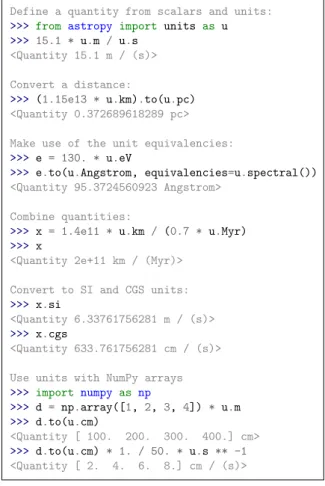
This sub-package includes the concept of “equivalencies” in units, which is intended to be used where there exists an equa-tion that provides a relaequa-tionship between two different physical quantities. A standard astronomical example is the relationships between the frequency, wavelength and energy of a photon – it is common practice to treat such units as equivalent even though they are not strictly comparable. Such a conversion can be car-ried out in astropy.units by supplying an equivalency list (see Fig.1). The inclusion of these equivalencies is an impor-tant improvement over existing unit-handling software, which typically does not have this functionality. Equivalencies are also included for monochromatic flux densities, which allows users to convert between Fν and Fλ, and users can easily implement their own equivalencies.
There are multiple string representations for units used in the astronomy community. The flexible image trans-port system (FITS) standard (Pence et al. 2010) defines a unit standard, as well as both the Centre de Données as-tronomiques de Strasbourg (CDS; Ochsenbein 2000) and NASA/Goddard’s Office of Guest Investigator Programs (OGIP;
George & Angelini 1995). In addition, the International Virtual
Observatory Alliance (IVOA) has a forthcoming VOUnit stan-dard (Derriere et al. 2012) in an attempt to resolve some of these differences. Rather than choose one of these, astropy.units supports most of these standards (OGIP support is planned for the next major release of astropy), and allows the user to se-lect the appropriate one when reading and writing unit string definitions to and from external file formats.
Define a quantity from scalars and units:
>>> from astropy import units as u
>>> 15.1 * u.m / u.s
<Quantity 15.1 m / (s)> Convert a distance:
>>> (1.15e13 * u.km).to(u.pc)
<Quantity 0.372689618289 pc> Make use of the unit equivalencies:
>>> e = 130. * u.eV
>>> e.to(u.Angstrom, equivalencies=u.spectral())
<Quantity 95.3724560923 Angstrom> Combine quantities:
>>> x = 1.4e11 * u.km / (0.7 * u.Myr)
>>> x
<Quantity 2e+11 km / (Myr)> Convert to SI and CGS units:
>>> x.si
<Quantity 6.33761756281 m / (s)>
>>> x.cgs
<Quantity 633.761756281 cm / (s)> Use units with NumPy arrays
>>> import numpy as np >>> d = np.array([1, 2, 3, 4]) * u.m >>> d.to(u.cm) <Quantity [ 100. 200. 300. 400.] cm> >>> d.to(u.cm) * 1. / 50. * u.s ** -1 <Quantity [ 2. 4. 6. 8.] cm / (s)>
Fig. 1.Quantity conversion using the astropy.units sub-package.
2.1.2. Quantities and physical constants
While the previous section described the use of the astropy.units sub-package to manipulate the units themselves, a more common use-case is to attach the units to quantities, and use them together in expressions. The astropy.units package allows units to be attached to Python scalars, or NumPy arrays, producing Quantity objects. These objects support arithmetic with other numbers and Quantity objects while preserving their units. For multiplication and division, the resulting object will retain all units used in the expression. The final object can then be converted to a specified set of units or decomposed, effectively canceling and combining any equivalent units and returning a Quantity object in some set of base units. This is demonstrated in Fig.1.
Using the .to() method, Quantity objects can easily be converted to different units. The units must either be dimen-sionally equivalent, or users should pass equivalencies through the equivalencies argument (cf. Sect.2.1.1or Fig.1). Since Quantity objects can operate with NumPy arrays, it is very sim-ple and efficient to convert the units on large datasets.
The Quantity objects are used to define a number of useful astronomical constants included in astropy.constants, each with an associated unit (where applicable) and additional meta-data describing their provenance and uncertainties. These can be used along with Quantity objects to provide a convenient framework for computing any quantity in astronomy. Figure2
includes a simple example that shows how the gravitational force between two bodies can be calculated in Newtons using physical constants and user-specified quantities.
Access physical constants:
>>> from astropy importunits as u >>> from astropy importconstants as c >>> print c.G
Name = Gravitational constant Value = 6.67384e-11
Error = 8e-15 Units = m3 / (kg s2) Reference = CODATA 2010
Combine quantities and constants:
>>> F = (c.G * (3 * c.M_sun) * (2 * u.kg) / ... (1.5 * u.au) ** 2)
>>> F.to(u.N)
<Quantity 0.0158179542881 N>
Fig. 2.Using the astropy.constants sub-package. Table 1. Supported time scales for astropy.time
Scale Description
TAI International atomic time TCB Barycentric coordinate time TCG Geocentric coordinate time TDB Barycentric dynamical time TT Terrestrial time
UT1 Universal time
UTC Coordinated universal time
2.2. Time
The astropy.time package provides functionality for manipu-lating times and dates. Specific emphasis is placed on supporting time scales (e.g. UTC, TAI, UT1) and time formats or repre-sentations (e.g. JD, MJD, ISO 8601) that are used in astronomy
(Guinot & Seidelmann 1988;Kovalevsky 2001;Wallace 2011).
Examples of using this sub-package are provided in Fig.3. The most common way to use astropy.time is to create a Time object by supplying one or more input time values as well as the time format or representation and time scale of those values. The input time(s) can either be a single scalar such as "2010-01-01 00:00:00" or 2455348.5 or a sequence of such values; the format or representation specifies how to interpret the input values, such as ISO, JD, or Unix time; and the scale specifies the time standard used for the values, such as coordi-nated universal time (UTC), terrestial time (TT), or international atomic time (TAI). The full list of available time scales is given in Table1. Many of these formats and scales are used within astronomy, and it is especially important to treat the different time scales properly when converting between celestial coordi-nate systems. To facilitate this, the Time class makes the con-version to a different format such as Julian Date straightforward, as well as the conversion to a different time scale, for instance from UTC to TT. We note that the Time class includes support for leap seconds in the UTC time scale.
This package is based on a derived version of the Standards of Fundamental Astronomy (SOFA) time and calendar library4
(Wallace 2011). Leveraging the robust and well-tested SOFA
routines ensures that the fundamental time scale conversions are being computed correctly. An important feature of the SOFA time library which is supported by astropy.time is that each time is represented as a pair of double-precision (64-bit) floating-point values, which enables extremely high precision
A&A 558, A33 (2013)
Parse a date/time in ISO format and on the UTC scale
>>> from astropy.time import Time >>> t = Time("2010-06-01 00:00:00", ... format="iso", scale="utc") >>> t
<Time object: scale=’utc’ format=’iso’ vals=2010-06-01 00:00:00.000> Access the time in Julian Date format
>>> t.jd
2455348.5
Access the time in year:day:time format
>>> t.yday
’2010:152:00:00:00.000’ Convert time to the TT scale
>>> t.tt
<Time object: scale=’tt’ format=’iso’ vals=2010-06-01 00:01:06.184> Find the Julian Date in the TT scale
>>> t.tt.jd
2455348.5007660184
Fig. 3. Time representation and conversion using the astropy.time sub-package.
time computations. Using two 64-bit floating-point values allows users to represent times with a dynamic range of 30 orders of magnitude, providing for example times accurate to better than a nanosecond over timescales of tens of Gyr. All time scale con-versions are done by vectorized con-versions of the SOFA routines using Cython (Behnel et al. 2011), a Python package that makes it easy to use C code in Python.
2.3. Celestial coordinates
An essential element of any astronomy workflow is the manipulation, parsing, and conversion of astronomical co-ordinates. This functionality is provided in Astropy by the astropy.coordinates sub-package. The aim of this pack-age is to provide a common application programming inter-face (API) for Python astronomy packages that use coordinates, and to relieve users from having to (re)implement extremely common utilities. To achieve this, it combines API and im-plementation ideas from existing Python coordinates packages. Some aspects, such as coordinate transformation approaches from kapteyn (Terlouw & Vogelaar 2012) and class structures resembling astropysics (Tollerud 2012), have already been implemented. Others, such as the frames of palpy (Jenness &
Berry 2013) and pyast (Berry & Jenness 2012) or the ephemeris
system of pyephem (Rhodes 2011), are still under design for astropy. By combining the best aspects of these other pack-ages, as well as testing against them, astropy.coordinates seeks to provide a high-quality, flexible Python coordinates library.
The sub-package has been designed to present a natural Python interface for representing coordinates in computations, simplify input and output formatting, and allow straightforward transformation between coordinate systems. It also supports im-plementation of new or custom coordinate systems that work consistently with the built-in systems. A future design goal is to seamlessly support arbitrarily large data sets.
Parse coordinate string
>>> import astropy.coordinates as coords
>>> c = coords.ICRSCoordinates("00h42m44.3s +41d16m9s")
Access the RA/Dec values
>>> c.ra <RA 10.68458 deg> >>> c.dec <Dec 41.26917 deg> >>> c.ra.degrees 10.68458333333333 >>> c.ra.hms (0.0, 42, 44.299999999999784) Convert to Galactic coordinates
>>> c.galactic.l
<Angle 121.17431 deg>
>>> c.galactic.b
<Angle -21.57280 deg>
Create a separate object in Galactic coordinates
>>> from astropy importunits as u
>>> g = c.transform_to(coords.GalacticCoordinates) >>> g.l.format(u.degree, sep=":", precision=3)
’121:10:27.499’
Set the distance and view the cartesian coordinates
>>> c.distance = coords.Distance(770., u.kpc) >>> c.x 568.7128882165681 >>> c.y 107.30093596881028 >>> c.z 507.8899092486349
Query SIMBAD to get coordinates from object names
>>> m = coords.ICRSCoordinates.from_name("M32") >>> m
<ICRSCoordinates RA=10.67427 deg, Dec=40.86517 deg> Two coordinates can be used to get distances
>>> m.distance = coords.Distance(765., u.kpc) >>> m.separation_3d(c)
<Distance 7.36865 kpc>
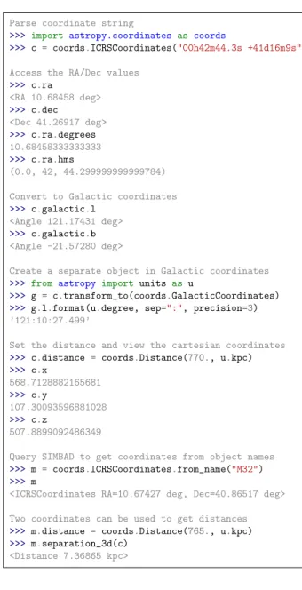
Fig. 4.Celestial coordinate representation and conversion.
Figure 4 shows some typical usage examples for astropy.coordinates. Coordinate objects are created using standard Python object instantiation via a Python class named after the coordinate system (e.g., ICRSCoordinates). Astronomical coordinates may be expressed in a myriad of ways: the classes support string, numeric, and tuple value specification through a sophisticated input parser. A design goal of the input parser is to be able to determine the angle value and unit from the input alone if a person can unambiguously determine them. For example, an astronomer seeing the input string 12h53m11.5123s would understand the units to be in hours, minutes, and seconds, so this value is alone sufficient to pass to the angle initializer. This functionality is built around the Angle object, which can be instantiated and used on its own. It provides additional functionality such as string formatting and mechanisms to specify the valid bounds of an angle. As a convenience, it is also possible to query the online SIMBAD5
database to resolve the name of a source (see Fig. 4 for an example showing how to find the ICRS coordinates of M 32).
5 http://simbad.u-strasbg.fr
The coordinate classes represent different coordinate sys-tems, and provide most of the user-facing functionality for astropy.coordinates. The systems provide customized ini-tializers and appropriate formatting and representation defaults. For some classes, they also contain added functionality spe-cific to a subset of systems, such as code to precess a coordi-nate to a new equinox. The implemented systems include a va-riety of equatorial coordinate systems (ICRS, FK4, and FK5), Galactic coordinates, and horizontal (Alt/Az) coordinates, and modern (IAU 2006/200A) precession/nutation models for the relevant systems. Coordinate objects can easily be transformed from one coordinate system to another: Fig.4illustrates the most basic use of this functionality to convert a position on the sky from ICRS to Galactic coordinates. Transformations are pro-vided between all coordinate systems built into version v0.2 of Astropy, with the exception of conversions from celestial to horizontal coordinates. Future versions of Astropy will in-clude additional common systems, including ecliptic systems, supergalactic coordinates, and all necessary intermediate coor-dinate systems for the IAU 2000/2006 equatorial-to-horizontal mapping (e.g.,Soffel et al. 2003;Kaplan 2005).
A final significant feature of astropy.coordinates is support for line-of-sight distances. While the term “celestial coordinates” can be taken to refer to only on-sky angles, in astropy.coordinates a coordinate object is conceptually treated as a point in three dimensional space. Users have the option of specifying a line of sight distance to the object from the origin of the coordinate system (typically the origin is the Earth or solar system barycenter). These distances can be given in physical units or as redshifts. The astropy.coordinates sub-package will in the latter case transparently make use of the cosmological calculations in astropy.cosmology (cf. Sect. 2.7) for conversion to physical distances. Figure 4 illus-trates an application of this information in the form of computing three-dimensional distances between two objects.
The astropy.coordinates sub-package was designed such that it should be easy for a user to add new coordinate systems. This flexibility is achieved in astropy.coordinates through the internal use of a transformation graph, which keeps track of a network of coordinate systems and the transforma-tions between them. When a coordinate object is to be trans-formed from one system into another, the package determines the shortest path on the transformation graph to the new system and applies the necessary sequence of transformations. Thus, implementing a new coordinate system simply requires imple-menting one pair of transformations to and from a system that is already connected to the transformation graph. Once this pair is specified, astropy.coordinates can transform from that coordinate system to any other in the graph. An example of a user-defined system is provided in the documentation6,
illustrat-ing the definition of a coordinate system useful for a specific scientific task.
2.4. Tables and Gridded data
Tables and n-dimensional data arrays are the most common forms of data encountered in astronomy. The Python community has various solutions for tables, such as NumPy structured ar-rays or DataFrame objects in Pandas (McKinney 2012) to name only a couple. For n-dimensional data the NumPy ndarray is the most popular.
6 http://docs.astropy.org/en/v0.2.4/coordinates/
sgr-example.html
Create an empty table and add columns
>>> from astropy.table import Table, Column >>> t = Table() >>> t.add_column(Column(data=["a", "b", "c"], ... name="source")) >>> t.add_column(Column(data=[1.2, 3.3, 5.3], ... name="flux")) >>> print t source flux -- ----a 1.2 b 3.3 c 5.3
Read a table from a file
>>> t1= Table.read("catalog.vot")
>>> t1= Table.read("catalog.tbl", format="ipac") >>> t1= Table.read("catalog.cds", format="cds")
Select all rows from t1 where the flux column is greater than 5
>>> t2= t1[t1["flux"] > 5.0]
Manipulate columns
>>> t2.remove_column("J_mag")
>>> t2.rename_column("Source", "sources")
Write a table to a file
>>> t2.write("new_catalog.hdf5", path=’/table’) >>> t2.write("new_catalog.rdb")
>>> t2.write("new_catalog.tex")
Fig. 5.Table input/output and manipulation using the astropy.table sub-package.
However, for use in astronomy all of these implementa-tions lack some key features. The data that is stored in ar-rays and tables often contains vital metadata: the data is as-sociated with units, and might also contain additional arrays that either mask or provide additional attributes to each cell. Furthermore, the data often includes a set of keyword-value pairs and comments (such as FITS headers). Finally, the data comes in a plethora of astronomy specific formats (FITS, spe-cially formatted ASCII tables, etc.), which are not recognized by the pre-existing packages.
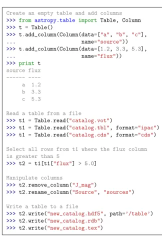
The astropy.table and astropy.nddata sub-packages contain classes (Table and NDData) that try to alleviate these problems. They allow users to represent astronomical data in the form of tables or n-dimensional gridded datasets, including all metadata. Examples of usage of astropy.table are shown in Fig.5.
The Table class provides a high-level wrapper to NumPy structured arrays, which are essentially arrays that have fields (or columns) with heterogeneous data types, and any number of rows. NumPy structured arrays are however difficult to mod-ify, so the Table class makes it easy for users to create a ta-ble from columns, add and remove columns or rows, and mask values from the table. Furthermore, tables can be easily read from and written to common file formats using the Table.read and Table.write methods. These methods are connected to sub-packages in astropy.io such as astropy.io.ascii (Sect. 2.5.2) and astropy.io.votable (Sect. 2.5.3), which allow ASCII and VO tables to be seamlessly read or written respectively.
In addition to providing easy manipulation and input or output of table objects, the Table class allows units to be
A&A 558, A33 (2013) specified for each column using the astropy.units framework
(Sect.2.1), and also allows the Table object to contain arbitrary metadata (stored in Table.meta).
Similarly, the NDData class provides a way to store n-dimensional array data easily and builds upon the NumPy ndarray class. The actual data is stored in an ndarray, which allows for easy compatibility with other scientific packages. In addition to keyword-value metadata, the NDData class can store a boolean mask with the same dimensions as the data, several sets of flags (n-dimensional arrays that store attributes for each cell of the data array), uncertainties, units, and a transforma-tion between array-index coordinate system and other coordinate systems (cf. Sect.2.6). In addition, the NDData class intends to provide methods to arithmetically combine the data in a mean-ingful way. NDData is not meant for direct user interaction but more for providing a framework for higher-level subclasses that can represent for example spectra or astronomical images.
2.5. File formats 2.5.1. FITS
Support for reading and writing FITS files is provided by the astropy.io.fits sub-package, which at the time of writing is a direct port of the PyFITS7project (Barrett & Bridgman 1999).
Users already familiar with PyFITS will therefore feel at home with this package.
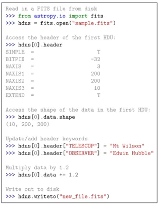
The astropy.io.fits sub-package implements all fea-tures from the FITS standard (Pence et al. 2010) such as images, binary tables, and ASCII tables, and includes common compres-sion algorithms. Header-data units (HDUs) are represented by Python classes, with the data itself stored using NumPy arrays, and with the headers stored using a Header class. Files can eas-ily be read and written, and once in memory can be easeas-ily mod-ified. This includes support for transparently reading from and writing to gzip-compressed FITS files as well as files using the tiled image compression standard. Figure6shows a simple ex-ample of how to open an existing FITS file, access and modify the header and data, and write a new file back to disk.
Creating new FITS files is also made simple. Since the code in this sub-package has been developed over more than a decade, it has been made to work with an extensive variety of FITS files, including ones that deviate from the FITS standard. This includes support for deprecated formats such as GROUPS HDUs as well as more obscure non-standard HDU types such as FITS HDUs which allow encapsulating multiple FITS files within FITS files. Support is also included for common but non-standard header conventions such as CONTINUE cards and ESO HIERARCH cards. Two command-line utilities for working with FITS files are packaged with Astropy: fitscheck can be used to validate FITS files against the standard. fitsdiff can be used to compare two FITS files on a number of criteria, and also in-cludes a powerful API for programmatically comparing FITS files.
Because the interface is exactly the same as that of PyFITS, users may directly replace PyFITS with Astropy in existing code by changing import statements such as import pyfits to from astropy.io import fits as pyfits without any additional code changes. Although PyFITS will continue to be released as a separate package in the near term, the long term plan is to discontinue PyFITS releases in favor of Astropy. It is expected that direct support of PyFITS will end mid-2014, so
7 http://www.stsci.edu/institute/software_hardware/
Read in a FITS file from disk
>>> from astropy.io import fits >>> hdus = fits.open("sample.fits")
Access the header of the first HDU:
>>> hdus[0].header SIMPLE = T BITPIX = -32 NAXIS = 3 NAXIS1 = 200 NAXIS2 = 200 NAXIS3 = 10 EXTEND = T
Access the shape of the data in the first HDU:
>>> hdus[0].data.shape
(10, 200, 200)
Update/add header keywords
>>> hdus[0].header["TELESCOP"] = "Mt Wilson"
>>> hdus[0].header["OBSERVER"] = "Edwin Hubble"
Multiply data by 1.2
>>> hdus[0].data *= 1.2
Write out to disk
>>> hdus.writeto("new_file.fits")
Fig. 6.Accessing data in FITS format.
users of PyFITS should plan to make suitable changes to support the eventual transition to Astropy.
Becoming integrated with Astropy as the astropy.io. fits sub-package will greatly enhance future development on the existing PyFITS code base in several areas. First and per-haps foremost is integration with Astropy’s Table interface (Sect. 2.4) which is much more flexible and powerful than PyFITS’ current table interface. We will also be able to inte-grate Astropy’s unit support (Sect.2.1) in order to attach units to FITS table columns as well as header values that specify units in their comments in accordance with the FITS standard. Finally, as the PyWCS package has also been integrated into Astropy as astropy.wcs (Sect.2.6), tighter association between data from FITS files and their WCS will be possible.
2.5.2. ASCII table formats
The astropy.io.ascii sub-package (formerly the standalone project asciitable8) provides the ability to read and write tab-ular data for a wide variety of ASCII-based formats. In addi-tion to generic formats such as space-delimited, tab-delimited or comma-separated values, astropy.io.ascii provides classes for specialized table formats such as CDS9, IPAC10, IRAF
DAOphot (Stetson 1987), and LaTeX. Also included is a flexible class for handling a wide variety of fixed-width table formats. Finally, this sub-package is designed to be extensible, making it easy for users to define their own readers and writers for any other ASCII formats.
8 https://asciitable.readthedocs.org 9 http://vizier.u-strasbg.fr/doc/catstd.htx 10 http://irsa.ipac.caltech.edu/applications/DDGEN/
2.5.3. Virtual Observatory (VO) tables
The astropy.io.votable sub-package (formerly the stan-dalone project vo.table) provides full support for reading and writing VOTable format files versions 1.1, 1.2, and the pro-posed 1.3 (Ochsenbein et al. 2004,2009). It efficiently stores the tables in memory as NumPy structured arrays. The file is read using streaming to avoid reading in the entire file at once and greatly reducing the memory footprint. VOTable files com-pressed using the gzip and bzip2 algorithms are supported trans-parently, as are VOTable files where the table data is stored in an external FITS file.
It is possible to convert any one of the tables in a VOTable file to a Table object (Sect.2.4), where it can be edited and then written back to a VOTable file without any loss of data.
The VOTable standard is not strictly adhered to by all VOTable file writers in the wild. Therefore, astropy.io.votable provides a number of tricks and workarounds to support as many VOTable sources as possible, whenever the result would not be ambiguous. A validation tool (volint) is also provided that outputs recommendations to improve the standard compliance of a given file, as well as validate it against the official VOTable schema.
2.6. World coordinate systems
The astropy.wcs sub-package contains utilities for managing WCS transformations in FITS files. These transformations map the pixel locations in an image to their real-world units, such as their position on the celestial sphere. This library is specific to WCS as it relates to FITS as described in the FITS WCS papers
(Greisen & Calabretta 2002;Calabretta & Greisen 2002;Greisen
et al. 2006) and is distinct from a planned Astropy package that
will handle WCS transformations in general, regardless of their representation.
This sub-package is a wrapper around the wcslib library11.
Since all of the FITS header parsing is done using wcslib, it is assured the same behavior as the many other tools that use wcslib. On top of the basic FITS WCS support, it adds support for the simple imaging polynomial (SIP) convention and table lookup distortions (Calabretta et al. 2004; Shupe et al. 2005). Each of these transformations can be used independently or to-gether in a fixed pipeline. The astropy.wcs sub-package also serves as a useful FITS WCS validation tool, as it is able to re-port on many common mistakes or deviations from the standard in a given FITS file.
As mentioned above, the long-term plan is to build a “gen-eralized” WCS for mapping world coordinates to image coordi-nates (and vice versa). While only in early planning stages, such a package would aim to not be tied to the FITS representation used for the current astropy.wcs. Such a package would also include closer connection to other parts of Astropy, for example astropy.coordinates (Sect.2.3).
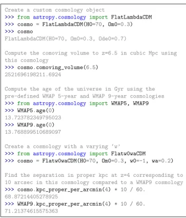
2.7. Cosmology
The astropy.cosmology sub-package contains classes for rep-resenting widely used cosmologies, and functions for calculat-ing quantities that depend on a cosmological model. It also con-tains a framework for working with less frequently employed cosmologies that may not be flat, or have a time-varying pres-sure to density ratio, w, for dark energy. The quantities that can
11 http://www.atnf.csiro.au/people/mcalabre/WCS/
Create a custom cosmology object
>>> from astropy.cosmology import FlatLambdaCDM >>> cosmo= FlatLambdaCDM(H0=70, Om0=0.3) >>> cosmo
FlatLambdaCDM(H0=70, Om0=0.3, Ode0=0.7)
Compute the comoving volume to z=6.5 in cubic Mpc using this cosmology
>>> cosmo.comoving_volume(6.5)
2521696198211.6924
Compute the age of the universe in Gyr using the pre-defined WMAP 5-year and WMAP 9-year cosmologies
>>> from astropy.cosmology import WMAP5, WMAP9 >>> WMAP5.age(0)
13.723782349795023
>>> WMAP9.age(0)
13.768899510689097
Create a cosmology with a varying ‘w’
>>> from astropy.cosmology import Flatw0waCDM
>>> cosmo= Flatw0waCDM(H0=70, Om0=0.3, w0=-1, wa=0.2)
Find the separation in proper kpc at z=4 corresponding to 10 arcsec in this cosmology compared to a WMAP9 cosmology
>>> cosmo.kpc_proper_per_arcmin(4) * 10 / 60.
68.87214405278925
>>> WMAP9.kpc_proper_per_arcmin(4) * 10 / 60.
71.21374615575363
Fig. 7.Cosmology utilities.
be calculated are generally taken from those described byHogg
(1999). Some examples are the angular diameter distance, co-moving distance, critical density, distance modulus, lookback time, luminosity distance, and Hubble parameter as a function of redshift.
The fundamental model for this sub-package is that any given cosmology is represented by a class. An instance of this class has attributes giving all the parameters required to specify the cosmology uniquely, such as the Hubble parameter, CMB temperature and the baryonic, cold dark matter, and dark energy densities at z = 0. One can then use methods of this class to perform calculations using these parameters.
Figure7shows how the FlatLambdaCDM class can be used to create an object representing a flatΛCDM cosmology, and how the methods of this object can be called to calculate the co-moving volume, age and transverse separation at a given red-shift. Further calculations can be performed using the many methods of the cosmology object as described in the Astropy documentation. For users who are more comfortable using a procedural coding style, these methods are also available as functions that take a cosmology class instance as a keyword argument.
The sub-package provides several pre-defined cosmology in-stances corresponding to commonly used cosmological parame-ter sets. Currently parameparame-ters from the WMAP 5-year (Komatsu
et al. 2009), 7-year (Komatsu et al. 2011) and 9-year results
(Hinshaw et al. 2012) are included (the WMAP5, WMAP7, and
WMAP9 classes). The parameters from the Planck results (Planck
Collaboration 2013) will be included in the next release of
Astropy. There are several classes corresponding to non-flat cos-mologies, and the most common dark energy models are sup-ported: a cosmological constant, constant w, and w(a) = w0+
wa(1 − a) (e.g.Chevallier & Polarski 2001;Linder 2003, here a
is the scale factor). Figure7gives examples showing how to use the pre-defined cosmologies, and how to define a new cosmology
A&A 558, A33 (2013) with a time-varying dark energy w(a). Any other arbitrary
mology can be represented by sub-classing one of the basic cos-mology classes.
All of the code in the sub-package is tested against the web-based cosmology calculator by Wright (2006) and two other widely-used calculators12,13. In cases when these calculators are
not precise enough to enable a meaningful comparison, the code is tested against calculations performed with M. 3. Development approach
A primary guiding philosophy of Astropy is that it is developed for and (at least in part) by the astronomy user community. This ensures the interface is designed with the workflow of working astronomers in mind. At the same time, it aims to make use of the expertise of software developers to design code that encour-ages good software practices such as a consistent and clean API, thorough documentation, and integrated testing. It is also ded-icated to remaining open source to enable wide adoption and render input from all users easier, and is thus released with a 3-clause BSD-style license (a license of this sort is “permis-sive” in that it allows usage of the code for any purposes as long as notice of the Astropy copyright and disclaimers of warranty are given). Achieving these aims requires code collaboration be-tween over 30 geographically-distributed developers, and here we describe our development workflow with the hope that it may be replicated by other astronomy software projects that are likely to have similar needs.
To enable this collaboration, we have made use of the GitHub14 open source code hosting and development platform.
The main repository for astropy is stored in a git15repository
on GitHub, and any non-trivial changes are made via pull re-quests, which are a mechanism for submitting code for review by other developers prior to merging into the main code base. This workflow aids in increasing the quality, documentation and testing of the code to be included in astropy. Not all contribu-tions are necessarily accepted – community consensus is needed for incorporating major new functionality in astropy, and any new feature has to be justified to avoid implementing features that are only useful to a minority of users, but may cause issues in the future.
At the time of writing, astropy includes several thousand tests, which are small units of code that check that functions, methods, and classes in astropy are behaving as expected, both in terms of scientific correctness and from a programming inter-face perspective. We make use of continuous integration, which is the process of running all the tests under various configura-tions (such as different versions of Python or NumPy, and on dif-ferent platforms) in order to ensure that the package is held to the highest standard of stability. In particular, any change made via a pull request is subject to extensive testing before being merged into the core repository. For the latter, we make use of Travis16, while for running more extensive tests across Linux, MacOS X, and Windows, we make use of Jenkins17 (both are examples of continuous integration systems).
This development workflow has worked very well so far, al-lowing contributions by many developers, and blurring the line
12 http://www.kempner.net/cosmic.php 13 http://www.icosmos.co.uk 14 http://www.github.com 15 http://git-scm.com 16 https://travis-ci.org 17 http://jenkins-ci.org
between developers and users. Indeed, users who encounter bugs and who know how to fix them can submit suggested changes. We have also implemented a feature that means that anyone reading the documentation athttp://docs.astropy.orgcan suggest improvements to the documentation with just a few clicks in a web browser without any prior knowledge of the git version control system.
4. Planned functionality
Development on the Astropy package is very active, and in ad-dition to some of the incremental improvements to existing sub-packages described in the text, we are focusing on implement-ing major new functionality in several areas for the next (v0.3) release (some of which have already been implemented in the publicly-available developer version):
– improving interoperability between packages, which includes for example seamlessly integrating the astropy.units framework across all sub-packages; – adding support for NumPy arrays in the coordinates
sub-package, which will allow the efficient representation and conversions of coordinates in large datasets;
– supporting more file formats for reading and writing Table and NDData objects;
– implementing a VO cone search tool (Williams et al. 2011); – implementing a generalized model-fitting framework; – implementing statistical functions commonly used in
Astronomy.
In the longer term, we are already planning the following major functionality:
– image analysis tools, including aperture and point spread function (PSF) photometry;
– spectroscopic analysis tools;
– generalized WCS transformations beyond the FITS WCS standard;
– a SAMP server/client (ported from the SAMPy18package);
– support for the Simple Image Access Protocol (SIAP;Tody
et al. 2011);
– support for the Table Access Protocol (TAP; Louys et al. 2011) is under consideration.
and undoubtedly the core functionality will grow beyond this. In fact, the astropy package will likely remain a continuously-evolving package, and will thus never be considered “complete” in the traditional sense.
5. Summary
We have presented the first public release of the Astropy pack-age (v0.2), a core Python packpack-age for astronomers. In this paper we have described the main functionality in this release, which includes:
– Units and unit conversions (Sect.2.1). – Absolute dates and times (Sect.2.2). – Celestial coordinate systems (Sect.2.3). – Tabular and gridded data (Sect.2.4).
– Support for common astronomical file formats (Sect.2.5). – WCS transformations (Sect.2.6).
– Cosmological calculations (Sect.2.7).
18 http://pythonhosted.org/sampy
We also briefly described our development approach (Sect. 3), which has enabled an international collaboration of scientists and software developers to create and contribute to the pack-age. We outlined our plans for the future (Sect. 4) which in-cludes more interoperability of sub-packages, as well as new functionality.
We invite members of the community to join the effort by adopting the Astropy package for their own projects, reporting any issues, and whenever possible, developing new functionality.
Acknowledgements. We thank the referee, Igor Chiligarian, for suggestions that helped improve this paper. We would like to thank the NumPy, SciPy (Jones et al. 2001), IPython and Matplolib communities for providing their packages which are invaluable to the development of Astropy. We thank the GitHub (http: //www.github.com) team for providing us with an excellent free develop-ment platform. We also are grateful to Read the Docs (https://readthedocs. org/), Shining Panda (https://www.shiningpanda-ci.com/), and Travis (https://www.travis-ci.org/) for providing free documentation hosting and testing respectively. Finally, we would like to thank all the astropy users that have provided feedback and submitted bug reports. The contribution by T. Aldcroft and D. Burke was funded by NASA contract NAS8-39073. The name resolution functionality shown in Fig.4makes use of the SIMBAD database, operated at CDS, Strasbourg, France.
References
Barrett, P. E., & Bridgman, W. T. 1999, in Astronomical Data Analysis Software and Systems VIII, ASP Conf. Ser., 172, 483
Behnel, S., Bradshaw, R., Citro, C., et al. 2011, Computing in Science Engineering, 13, 31
Berry, D. S., & Jenness, T. 2012, in Astronomical Data Analysis Software and Systems XXI, eds. P. Ballester, D. Egret, & N. P. F. Lorente, ASP Conf. Ser., 461, 825
Calabretta, M. R., & Greisen, E. W. 2002, A&A, 1077
Calabretta, M. R., Valdes, F., Greisen, E. W., & Allen, S. L. 2004, in Astronomical Data Analysis Software and Systems (ADASS) XIII, eds. F. Ochsenbein, M. G. Allen, & D. Egret, ASP Conf. Ser., 314, 551
Chevallier, M., & Polarski, D. 2001, Int. J. Mod. Phys. D, 10, 213
Derriere, S., Gray, N., Louys, M., et al. 2012, Units in the VO, Version 1.0, IVOA Proposed Recommendation 20 August 2012 ed.
George, I., & Angelini, L. 1995, Specification of Physical Units within OGIP (Office of Guest Investigator Programs) FITS files
Greenfield, P. 2011, in Astronomical Data Analysis Software and Systems XX, eds. I. N. Evans, A. Accomazzi, D. J. Mink, & A. H. Rots, ASP Conf. Ser., 442, 425
Greisen, E. W., & Calabretta, M. R. 2002, A&A, 1061
Greisen, E. W., Calabretta, M. R., Valdes, F. G., & Allen, S. L. 2006, A&A, 747
Guinot, B., & Seidelmann, P. K. 1988, A&A, 194, 304
Hinshaw, G., Larson, D., Komatsu, E., et al. 2012 [arXiv:1212.5226] Hogg, D. W. 1999, ArXiv Astrophysics e-prints [arXiv:astro-ph/9905116] Jenness, T., & Berry, D. S. 2013, in ADASS XXII, eds. D. Friedel, M. Freemon,
& R. Plante (San Francisco: ASP), ASP Conf Ser., TBD, in press Jones, E., Oliphant, T., & Peterson, P. 2001,http://www.scipy.org/ Kaplan, G. H. 2005, US Naval Observatory Circulars, 179
Komatsu, E., Dunkley, J., Nolta, M. R., et al. 2009, ApJS, 180, 330 Komatsu, E., Dunkley, J., Nolta, M. R., et al. 2011, ApJS, 192, 18
Kovalevsky, J. 2001, in Journées 2000 – systèmes de référence spatio-temporels. J2000, a fundamental epoch for origins of reference systems and astronomical models, ed. N. Capitaine, 218
Linder, E. V. 2003, Phys. Rev. Lett., 90, 091301
Louys, M. Bonnarel, F., Shade, D., et al. 2011 [arXiv:1111.1758]
McKinney, W. 2012, Python for Data Analysis (O’Reilly Media, Incorporated) Ochsenbein, F. 2000, Astronomical Catalogues and Tables Adopted Standards,
Version 2.0
Ochsenbein, F., et al. 2004, VOTable Format Definition, Version 1.1, International Virtual Observatory Alliance (IVOA)
Ochsenbein, F., Davenhall, C., Durand, D., et al. 2009, VOTable Format Definition, Version 1.2, International Virtual Observatory Alliance (IVOA) Oliphant, T. 2006, A Guide to NumPy, 1 (Trelgol Publishing USA)
Pence, W. D., Chiappetti, L., Page, C. G., Shaw, R. A., & Stobie, E. 2010, A&A, 524, A42
Planck Collaboration 2013, A&A, submitted [arXiv:1303.5076]
Pontzen, A., Roškar, R., Stinson, G. S., et al. 2013, Pynbody: Astrophysics Simulation Analysis for Python (Astrophysics Source Code Library, ascl:1305.002)
Rhodes, B. C. 2011, PyEphem: Astronomical Ephemeris for Python (Astrophysics Source Code Library, ascl:1112.014)
Shupe, D. L., Moshir, M., Li, J., et al. 2005, in Astronomical Data Analysis Software and Systems XIV, eds. P. Shopbell, M. Britton, & R. Ebert, ASP Conf. Ser., 347, 491
Soffel, M., Klioner, S. A., Petit, G., et al. 2003, AJ, 126, 2687 Stetson, P. B. 1987, PASP, 99, 191
Terlouw, J. P., & Vogelaar, M. G. R. 2012, Kapteyn Package, version 2.2, Kapteyn Astronomical Institute, Groningen
Tody, D., Plante, R., & Harrison, P. 2011 [arXiv:1110.0499]
Tollerud, E. 2012, Astropysics: Astrophysics utilities for python (Astrophysics Source Code Library, ascl:1207.007)
Van Der Walt, S., Colbert, S., & Varoquaux, G. 2011, Computing in Science & Engineering, 13, 22
Wallace, P. T. 2011, Metrologia, 48, 200
Williams, R., Hanisch, R., Szalay, A., & Plante, R. 2011 [arXiv:1110.0498] Wright, E. L. 2006, PASP, 118, 1711