HAL Id: hal-01946507
https://hal.archives-ouvertes.fr/hal-01946507
Submitted on 27 Nov 2020
HAL is a multi-disciplinary open access
archive for the deposit and dissemination of
sci-entific research documents, whether they are
pub-lished or not. The documents may come from
teaching and research institutions in France or
abroad, or from public or private research centers.
L’archive ouverte pluridisciplinaire HAL, est
destinée au dépôt et à la diffusion de documents
scientifiques de niveau recherche, publiés ou non,
émanant des établissements d’enseignement et de
recherche français ou étrangers, des laboratoires
publics ou privés.
house mouse hybrid zone
Nathalie Raufaste, Annie Orth, Khalid Belkhir, David Senet, Carole Smadja,
Stuart Baird, François Bonhomme, Barbara Dod, Pierre Boursot
To cite this version:
Nathalie Raufaste, Annie Orth, Khalid Belkhir, David Senet, Carole Smadja, et al.. Inferences of
selection and migration in the Danish house mouse hybrid zone. Biological Journal of the Linnean
Society, Linnean Society of London, 2005, 84 (3), pp.593-616. �hal-01946507�
Biological Journal of the Linnean Society
, 2005,
84
, 593–616. With 5 figures
Blackwell Science, LtdOxford, UKBIJBiological Journal of the Linnean Society0024-4066The Linnean Society of London, 2005? 2005 843
593616 Original Article
SELECTION IN THE HOUSE MOUSE HYBRID ZONE N. RAUFASTE
Et al.
*Corresponding author. E-mail: [email protected]
†Present address: INRA CBGP, Campus de Baillarguet, 34988
Montferrier sur Lez, France
The genus Mus as a model for evolutionary studies
Edited by J. Britton-Davidian and J. B. Searle
Inferences of selection and migration in the Danish house
mouse hybrid zone
NATHALIE RAUFASTE
1
, ANNIE ORTH
1
, KHALID BELKHIR
1
, DAVID SENET
1
,
CAROLE SMADJA
2
, STUART J. E. BAIRD
1†
, FRANÇOIS BONHOMME
1
, BARBARA DOD
1
and PIERRE BOURSOT
1
*
1
Laboratoire Génome Populations Interactions Adaptation (UMR 5171 IFREMER-CNRS-UMII), and
2
Institut des Sciences de l’Evolution (UMR 5554 CNRS-UMII), Université Montpellier II, France
Received 30 October 2003; accepted for publication 7 October 2004
We analysed the patterns of allele frequency change for ten diagnostic autosomal allozyme loci in the hybrid zone
between the house mouse subspecies
Mus musculus domesticus
and
M. m. musculus
in central Jutland. After
deter-mining the general orientation of the clines of allele frequencies, we analysed the cline shapes along the direction of
maximum gradient. Eight of the ten clines are best described by steep central steps with coincident positions and an
average width of 8.9 km (support limits 7.6–12.4) flanked by tails of introgression, indicating the existence of a
bar-rier to gene flow and only weak selection on the loci studied. We derived estimates of migration from linkage
dise-quilibrium in the centre of the zone, and by applying isolation by distance methods to microsatellite data from some
of these populations. These give concordant estimates of
s
=
0.5–0.8 km generation
–. The barrier to gene flow is of
the order of 20 km (support limits 14–28), and could be explained by selection of a few per cent at 43–120
under-dominant loci that reduces the mean fitness in the central populations to 0.45. Some of the clines appear
symmet-rical, whereas others are strongly asymmetsymmet-rical, and two loci appear to have escaped the central barrier to gene flow,
reflecting the differential action of selection on different parts of the genome. Asymmetry is always in the direction
of more introgression into
musculus
, indicating either a general progression of
domesticus
into the
musculus
terri-tory, possibly mediated by differential behaviour, or past movement of the hybrid zone in the opposite direction,
impeded by potential geographical barriers to migration in
domesticus
territory.
© 2005 The Linnean Society of
London,
Biological Journal of the Linnean Society
, 2005,
84
, 593–616.
ADDITIONAL KEYWORDS:
gene flow – genetic barrier – hybridization –
Mus musculus domesticus
–
Mus
musculus musculus
– speciation.
1
/
2INTRODUCTION
Hybrid zones have been referred to as ‘windows on
the evolutionary process’ (Harrison, 1990) because
they allow us to study the interplay between
migra-tion and selecmigra-tion on the evolumigra-tion of genetic
differen-tiation and adaptation. When parapatric taxa meet
and hybridize, selection against unfit hybrids can
counteract the homogenizing effect of migration and
lead to the establishment of frequency clines of
diag-nostic characters at the boundary between their
dis-tribution areas. A detailed population genetics theory
has been developed to model the expected patterns of
allele frequency changes in such situations (e.g. for
reviews see Barton & Hewitt, 1985; Barton & Gale,
1993), showing that they can constitute barriers to
gene flow between the taxa, of increasing intensity
with the number of loci involved in hybrid unfitness,
and with the spread of these loci in the genome.
594
N. RAUFASTE
ET AL
.
Briefly, this is because migration brings parental
gen-otypes to the centre of the hybrid zone where neutral
loci are thus in linkage disequilibrium with loci under
selection in hybrids, which impedes free introgression
of these neutral loci and causes an abrupt change of
their allele frequency in the centre. However, these
loci can eventually extricate themselves from this
negative genetic background by recombination, and
form long tails of introgression into the foreign
terri-tory. The resulting clines (described by the shapes of
the central step and of the tails of introgression) are
relatively independent of the type of selection against
hybrids (which is usually unknown), and can be used
to quantify the intensity of the selection maintaining
the zone and of the resulting barrier to gene flow.
Their estimation can also provide some information
about the number of loci involved in the selection of
hybrids, an important characteristic of the
mecha-nisms leading to incompatibilities between
differenti-ating genomes.
Since the pioneering work of Hunt & Selander
(1973), several authors have studied the genetics of
the hybrid zone between the two European subspecies
of the house mouse,
Mus musculus domesticus
and
M. m. musculus
, that are thought to have come into
secondary contact in Europe after a period of
indepen-dent geographical expansion from the Middle East,
with
M. m. domesticus
colonizing the Mediterranean
basin and Western Europe while
M. m. musculus
was
expanding across central Europe (e.g. see Boursot
et al
., 1993, for a review). In previous studies, cline
widths were roughly quantified by visually inspecting
the variations of synthetic morphological or genetic
hybrid indexes: 90% of the genetic transition occurs
over 20 km in Denmark (Hunt & Selander, 1973), 75%
over 20 km in southern Germany (Sage, Whitney &
Wilson, 1986b), 80% over 36 km in Bulgaria
(Vanler-berghe
et al
., 1988), and 60% of genetic and
morpho-logical variation in 20–40 km in East Holstein (Prager
et al.
, 1993). The first attempt to estimate cline widths
involved the application of a simple sigmoid model on
the south German transect (Tucker
et al
., 1992). They
found narrower cline widths for the sex chromosome
markers (Y chromosome, 4 km; X chromosome
mark-ers from 4 to 10 km) compared with autosomal
alloz-ymes (from 6.4 to 21.2
km). A similar contrast
between the sex chromosomes and autosomal loci was
also found in Denmark and Bulgaria (Vanlerberghe
et al
., 1986; Dod
et al
., 1993). However, none of these
studies had enough samples both in the centre and in
the tails of introgression for a detailed analysis of the
cline shape to be realistic. In addition, sampling was
often carried out in a linear fashion in an arbitrary
direction across the transect, allowing comparisons
between markers, but not the calculation of cline
parameters along the line of maximum slope.
Further-more, none of these studies included estimations of
migration, nor of linkage disequilibrium that could be
combined with cline widths to estimate the intensity
of selection against hybrid mice. Here we analyse a
large dataset on the Danish hybrid zone characterized
for ten diagnostic allozyme loci, and derive
indepen-dent estimates of migration using microsatellite loci.
MATERIAL AND METHODS
M
ICE
Mice were live trapped inside buildings using
multi-capture wire traps, during several field trips from
1984 to 2000. The location of the sampling sites in the
Jutland peninsula is indicated on Figure 1 and the list
of localities with their Universal Transverse Mercator
(UTM) coordinates are given in Appendix 1.
P
ROTEIN
ELECTROPHORESIS
Mice were killed and dissected in the field, and liver,
kidney, heart, plasma and blood cells were kept in
liq-uid nitrogen for further preparations. Protein
extrac-tions, separation by starch gel electrophoresis (or
acrylamide gels in the case of Amylase) and detection
of enzyme activity in the gels followed standard
pro-tocols, such as described in Pasteur
et al
. (1987). The
loci were chosen for their ability to distinguish
between the two subspecies in previous studies on
house mice in the Jutland peninsula and on a broader
geographical scale (Hunt & Selander, 1973;
Bonho-mme
et al
., 1984; Britton-Davidian, 1990; Din
et al
.,
1996). The alleles were identified by comparison with
standards obtained from mice of known genotypes,
and each locality was characterized by the frequency
of
M. m. musculus
alleles.
O
RIENTATION
OF
THE
CLINES
The general orientation of the maximum gradient of
allele frequency across the hybrid zone was
deter-mined by fitting the allele frequency data to a simple
sigmoid model, where the logit transform of the allele
frequencies is a linear function of the
two-dimen-sional (2D) geographical coordinates. The model was
fitted by maximum likelihood, assuming a binomial
error on the estimations of allele frequencies, using
the computer package GLIM4 (the Numerical
Algo-rithm Group). This orientation procedure determined
the direction of maximum gradient of allele
fre-quency, assuming the centre of the hybrid zone is a
straight line, and that the frequency change is
sig-moid. The coordinate of each locality was then
calcu-lated by projection on this direction of maximum
gradient.
SELECTION IN THE HOUSE MOUSE HYBRID ZONE
595
F
ITTING
CLINE
SHAPE
The
musculus
allele frequencies for each locus in the
different localities along the 1D transect were fitted to
various models of cline shapes by maximum likelihood
estimation, using the computer package Analyse
(by N. Barton & S. Baird, http://helios.bto.ed.ac.uk/
evolgen/Mac/Analyse/).
Sample sizes were corrected according to:
(1)
(adapted from Szymura & Barton, 1986, 1991), where
N
is the number of individuals sampled in the locality.
F
ISis the deficit of heterozygotes (set to zero if not
pos-itive) and is used to correct for the non-independence
between sampling of alleles when there is inbreeding.
F
STrepresents the fluctuations of allele frequencies
between loci that are not accounted for by differences
in their cline shapes. It represents the residual
varia-tion around the regression of allele frequencies at
individual loci in each locality against the average of
all loci, and was estimated using the ‘concordance’
procedure in the Analyse package. The above
correc-tion is designed for a single locus. When data for
sev-Ne
N
N
Fst
Fis
=
+
+
2
2
*
1
eral loci were pooled, the effective sample size was
taken as the sum of effective sample sizes for the
dif-ferent loci.
The Analyse package is then used to compare the
likelihood of the allele frequency data under three
dif-ferent models of cline shape: a sigmoid cline, and
clines in three parts, with a central sigmoid part and
two exponential tails of introgression, either identical
on both sides or different. The first model has two
parameters,
w
, the width of the cline (inverse of the
maximum slope), and
c
, the geographical position of
the centre. The second model has two additional
parameters (four in total) describing the shape of the
exponential tails, and the last model has two such
parameters for each tail (six parameters in total). As
the models are nested, a likelihood ratio test can be
applied to choose the model that best explains the data
with a minimum of parameters, by assuming that
twice the difference of log-likelihood between two
mod-els follows a chi-squared distribution with the number
of degrees of freedom equal to the difference in the
number of parameters between the two models.
The Analyse program uses a Metropolis random
exploration algorithm to find the maximum likelihood
Figure 1.
Location of the sampling sites are shown by open triangles on the map, and the axes give their UTM coordinates.
Inset: the location of the study area in the Jutland Peninsula. The grey line running across the map is the position of the
centre of the hybrid zone that ends in the east at the head of the Vejle Fjord. The rivers are drawn on this map, and some
are highlighted by thicker lines (see text).
6120
6140
6160
6180
6200
6220
475
495
515
535
555
575
10 km
N
596
N. RAUFASTE
ET AL
.
estimate of the parameters, so it was run many times
on each dataset, with different starting conditions and
different settings of the parameters controlling the
exploration algorithm, in order to explore the
param-eter space as thoroughly as possible. Two
log-likelihood support limits of parameter estimates were
determined by inspecting the results of 10 000–50 000
explorations of the parameter space with the
algo-rithm. The likelihood profiles (Hilborn & Mangel,
1997) for position and width were explored using the
‘crossection’ option of Analyse, as described in
Phil-lips, Baird & Moritz (2004): the parameter of interest
(
c
or
w
) is set to a fixed value, and the other
parame-ters are searched until the maximum likelihood of the
data is found for this value of
c
(
w
). The procedure is
repeated for a range of values of
c
(
w
) until the range
of relevant values is covered, and the likelihood profile
can thus be generated for the parameter of interest.
E
STIMATING
SELECTION
PARAMETERS
The parameters of the fitted cline shapes can be used
to infer some population parameters of interest, using
the existing theory of tension zones, as detailed in a
number of papers (Barton & Hewitt, 1985; Szymura &
Barton, 1986, 1991; Barton & Gale, 1993; Kruuk
et al
.,
1999; Barton & Shpak, 2000). We will summarize here
the part of this complex theory that was used.
As we will see, a cline shape in three parts, with a
central sigmoid part and two exponential tails, best
describes most loci studied. This is the shape expected
for a locus under weak selection (creating the
expo-nential tails of introgression) submitted to the
influ-ence of several loci under stronger selection, creating
the central barrier to gene flow, and the central step in
the clines. Although some of the theory summarized
below is derived for neutral loci, the hypothesis of
weak selection on the studied loci needs to be
intro-duced to derive equilibrium cline shapes (the only
equilibrium for neutral loci would be even frequency,
e.g. Szymura & Barton, 1986, 1991).
The central sigmoid step can be described by two
parameters,
c
, the position of the centre, and
w
, the
width of the cline (inverse of the maximum slope). The
following relation relates the total selection acting on
the locus to the width of the cline:
(2)
where
s
2is the migration parameter (variance of
dis-tance from parent to offspring). This is a nuisance
parameter, but it is possible to estimate it by
compar-ing the clines for different loci and their linkage
dise-quilibria. It is expected to be proportional to the
linkage disequilibrium and the rate of recombination
between the loci, and to the gradients of allele
fre-s
w
* =
8
2 2s
quencies for these loci. Standardized linkage
disequi-libria (linkage disequilibrium standardized by the
maximum possible value given allele frequencies)
between pairs of loci were estimated by maximum
likelihood with the program Analyse, in localities from
the centre of the hybrid zone, where linkage
disequi-librium is expected to be maximum, and where the
gradient of allele frequencies is estimated as the
inverse of cline width. The migration parameter was
estimated for each locality and each pair of loci. The
estimates obtained are then averaged over pairs of loci
and localities to obtain a single estimate of the
migra-tion parameter. Because the statistical properties of
such an average are not known, we also used the
vari-ance of the individual hybrid index to estimate the
average linkage disequilibrium between loci (Barton
& Gale, 1993),
—
D
.
The equations of the exponential tails of
introgres-sion allow the inference of other important
parame-ters. The equation of the left tail of the cline is:
(3)
and that of the right tail
(4)
It can be seen that parameters
q
represent the
square of the ratio between the expected rate of decay
in the tails without a barrier and the actual rate of
decay. They can thus be used to estimate the ratio
between the selection on the locus under study itself
and the total selection experienced by this locus,
including the influence of other loci:
(5)
The program Analyse does not give estimates of the
a
parameters but of parameters
B
/
w
, the ratio of the
barrier to gene flow to the width of the clines. The
rela-tionship between these parameters is:
(6)
and similarly for
B
1.
By making the hypothesis that selection on the loci
studied is weak, that the number of loci under
selec-tion is not too small (1/
n
<<
1) and that selection acts
against heterozygotes, one can derive approximate
estimates of the number of loci under selection
creat-ing the barrier and the intensity of the selection on
each locus using the two following relationships (e.g.
Barton & Shpak, 2000):
(7)
p x
x
c
w
( ) =
a
0Ê
Ë
(
-
)
q
0ˆ
¯
2
exp
,
p x
x
c
w
( ) = -
1
a
1exp
Ê
Ë
-
2
(
-
)
q
1¯
ˆ
.
q =
s
s
locus*
.
B
0w
0 0 1 02
1
=
-
-q
a
a
a
.
,
s
B
B
w u
=
8
Ê
Ë
ˆ
¯
2 2 2s
ln
and
D
(8)
where Du is the height of the central step of allele
quency, and is estimated as the difference in the
fre-quencies of the two exponential tails taken at the
centre (x = c). We thus have Du = 1 - a
0- a
1, which
becomes:
(9)
Note that in the literature, Du is sometimes omitted,
supposing that selection is strong and that it is close to
1 (Szymura & Barton, 1986, 1991).There remains one
nuisance parameter in the equations above, which is
r¯, the average recombination rate between the neutral
(or quasi-neutral in that case) locus and the loci under
selection. Several methods have been suggested to
estimate r¯ (Barton & Hewitt, 1985; Barton &
Bengts-son, 1986). Here we take the conservative value of 0.5
that gives the upper limit of n, the number of loci
under selection. In the framework of this
underdomi-nance model, the average fitness of the central
popu-lations can be estimated (taking the fitness of the
parental populations arbitrarily at 1):
(10)
M
ICROSATELLITE
TYPING
Genomic DNA was extracted from the spleen using
standard proteinase K/phenol-chloroform methods.
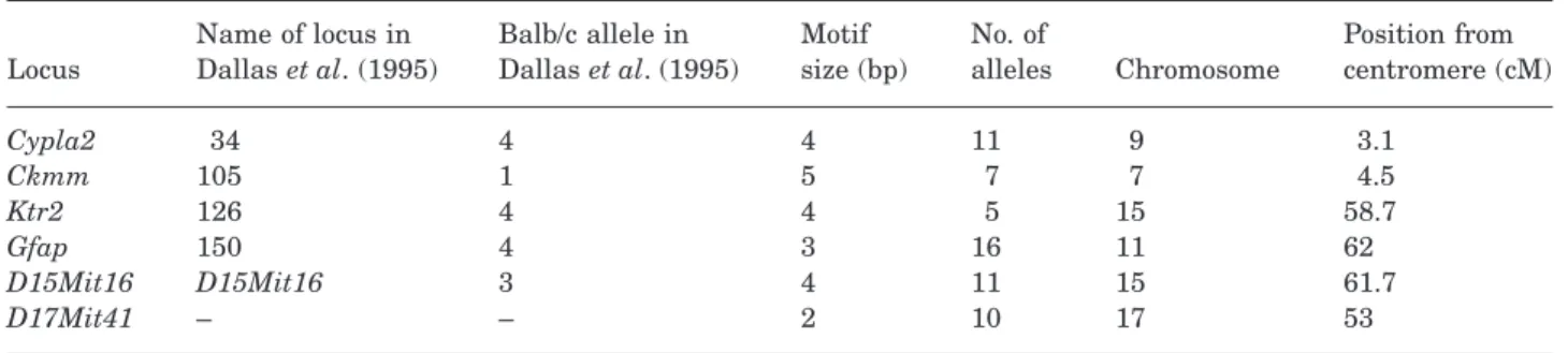
Polymorphism was studied at six microsatellite loci
that are described in Table 1. Five of them are
com-mon with the previous study of Dallas et al. (1995).
The loci were amplified by PCR. One of the
amplifica-tion primers was fluorescently labelled (Cy5) and
allele sizes were measured after migration in a
dena-turing acrylamide gel on an automated sequencer
n
r
B
B
w u
=
Ê
Ë
ˆ
¯
2s ln
D
Du
w
B
B
B
B
w
B
B
=
+
+
2
2
0 0 1 1 0 0 1 1 0 0 1 1q
q
q
q
q
q
.
W
H=
exp
Ê
Ë
-
ns
ˆ
¯
2
.
(Pharmacia). Allele sizes for all loci were measured
relative to the corresponding allele of the Balb/c
mouse laboratory strain, which was arbitrarily
attrib-uted size 50. We intentionally selected loci with 3–5-bp
repeats (except D17Mit41, 2 bp, Table 1), because
allele size determination is more reliable than for 2-bp
repeats.
E
STIMATION
OF
MIGRATION
FROM
MICROSATELLITE
ALLELE
FREQUENCIES
We estimated the migration parameter s under
isola-tion by distance models, using three different methods
applied to the microsatellite data. The first method
calculates the regression between FST
/(1 - FST) and
the logarithm of geographical distance between
lations, r (Rousset, 1997). It applies to pairs of
popu-lations in a 2D habitat, and the slope of the regression
gives an estimate of 1/4pDs
2, where D is the local
pop-ulation density, and s
2is the dispersion parameter. We
chose F
STrather than R
ST(Slatkin, 1995) because it is
thought to be more conservative when sample sizes
are small, and only a few loci are used (Gaggiotti et al.,
1999), but also because of its small variance and of the
uncertainties about the mutation model underlying
the justification of RST. The second method calculates
the regression of statistic
over the logarithm of
geo-graphical distance, r (Rousset, 2000b), the slope of
which also provides an estimate of 1/4pDs
2. Here,
however, pairs of individuals rather than of
popula-tions are compared, and statistic
is given by (Qw
Qr)/(1 - Qw), where Qr is the probability of identity by
state of two alleles separated by a distance r, and Q
wis
the probability of identity by state of the two alleles
from the same individual. The third method used here
calculates the regression of a spatial autocorrelation
statistic, Moran’s I, over the logarithm of geographical
distance r (Hardy & Vekemans, 1999). It also applies
to pairs of individuals, and the slope of the regression
can be used as an estimate of (1 - FIT)/2pDs
2(1 + FIT).
Computer software GENETIX
(http://www.univ-montp2.fr/~genetix/genetix/genetix.htm) was used to
)
a
r)
a
rTable 1. Description of the microsatellite loci studied
Locus
Name of locus in
Dallas et al. (1995)
Balb/c allele in
Dallas et al. (1995)
Motif
size (bp)
No. of
alleles
Chromosome
Position from
centromere (cM)
Cypla2
34
4
4
11
9
3.1
Ckmm
105
1
5
7
7
4.5
Ktr2
126
4
4
5
15
58.7
Gfap
150
4
3
16
11
62
D15Mit16
D15Mit16
3
4
11
15
61.7
D17Mit41
–
–
2
10
17
53
calculate FST and convert data files between different
formats, while GENEPOP (ver. 3.3, Raymond &
Rous-set, 1995) allowed the calculation of
. A program
was written to calculate Moran’s I, according to the
formula in Hardy & Vekemans (1999).
RESULTS
A
LLOZYME
ANALYSES
A total of 170 localities, listed in Appendix 1 with their
geographical coordinates, were studied here and their
location is indicated in Figure 1. Most yielded five
mice or fewer (see Appendix 1 and the distribution of
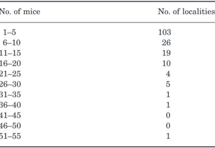
sample sizes in Table 2). The results of the genetic
analysis at the ten enzymatic autosomal loci (Amy,
Es1, Es10, Es2, Gpd, Idh, Mpi, Np, Pgm and Sod) are
given in Appendix 2. A total of 1233 mice were studied,
but only 996–1187 were successfully typed, depending
on the locus.
Samples from the same locality but different
collec-tion years were treated separately. An independent
study (to be published elsewhere) failed to find any
evidence that this hybrid zone has moved since it was
sampled in the late 1960s by Hunt & Selander (1973)
and our sampling period which extended from 1984 to
2000. We therefore considered here that the zone was
stable enough for us to analyse all sampling years
together, in order to increase the quality of the
sam-pling along the transect.
O
RIENTATION
OF
THE
TRANSECT
When fitting a sigmoid cline to the data in two
dimen-sions, the centre of the hybrid zone was found to run
west-north-west to east-south-east, at a 7∞ angle
clock-wise from the west–east direction (as drawn on the map
of Fig. 1). We will see below that most loci do not fit the
simple sigmoid cline model used here, but rather more
complex models with a central step of allele frequency.
)
a
rWe were thus concerned that the use of this simple
model could lead to an erroneous determination of the
direction of the clines. Using the more complex models,
we tested several orientations with angles from 0 to 20∞
and found in all cases that the 7∞ orientation gave the
best likelihood (data not shown). The coordinates of the
localities along the transect were thus calculated by
projecting them onto an axis perpendicular to this
cen-tral line. However, as can be seen on the map, the centre
of the hybrid zone reaches at its eastern end the head
of a deep fjord (the Vejle Fjord). For localities further
east of this point our standard procedure would
cer-tainly underestimate their distance to the centre of the
hybrid zone. Thus, the straight line distance between
the locality considered and the head of the fjord was
added to (north of the hybrid zone centre) or subtracted
from (south of the hybrid zone centre) the transect
coor-dinate of the head of the fjord. The amended transect
coordinates are listed in Appendix 1, and are used in
the following analyses.
C
LINE
SHAPES
The 1D coordinates of the localities calculated as
described above were used to analyse the shape of the
cline of allele frequency along the transect. The three
models implemented by the computer program
Anal-yse were fitted successively: sigmoid cline (two
param-eters), symmetric stepped cline (four parameters) and
asymmetric stepped cline (six parameters). The
likeli-hood ratio test was used to compare the models and
the choice was made at the 5% significance level.
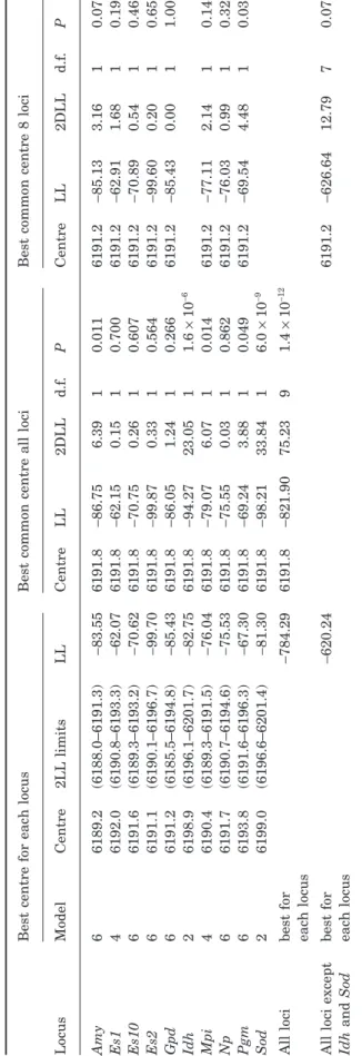
Table 3 shows the type of model retained for each
locus using this criterion. The sigmoid model (two
parameters) could not be rejected for Idh and Sod,
while a stepped symmetric model (four parameters)
was retained for Es1 and Mpi, but the stepped
asym-metric model (six parameters) provided the best fit for
the six remaining loci. The best positions of the
cen-tres for each locus and their 2 Log-Likelihood (LL)
support limits are given in Table 3. We then tested
whether an acceptable common centre for all loci could
be found. To do this, we calculated the best LL of each
locus dataset for a range of centres spanning the
con-fidence intervals of all loci, leaving all the other
parameters free to vary. We then summed the best LLs
over loci for each of the centres tested, and determined
the position that provides the best summed LL
(method described in Phillips et al., 2004). This model,
with a common centre at position 6191.8 (Table 3), is
significantly worse than that where the centre is free
to vary at each locus (P = 1.4 ¥ 10
-12). Inspection of the
individual tests for each locus between the free and
constrained centre models identifies two clear outliers
(Table 3): Idh and Sod, the two loci for which sigmoid
clines were retained. We reiterated the above
proce-Table 2. The distribution of sample sizes
No. of mice
No. of localities
1–5
103
6–10
26
11–15
19
16–20
10
21–25
4
26–30
5
31–35
1
36–40
1
41–45
0
46–50
0
51–55
1
T
able 3.
Maximum likelihood position of the centre for eac
h locus
, and the likelihood searc
h of a common centre
Locus
Best centre for eac
h locus
Best common centre all loci
Best common centre 8 loci
Model
Centre
2LL limits
LL
Centre
LL
2DLL
d.f
.
P
Centre
LL
2DLL
d.f
.
P
Amy
6
6189.2
(6188.0–6191.3)
-83.55
6191.8
-86.75
6.39
1
0.011
6191.2
-85.13
3.16
1
0.076
Es1
4
6192.0
(6190.8–6193.3)
-62.07
6191.8
-62.15
0.15
1
0.700
6191.2
-62.91
1.68
1
0.195
Es10
6
6191.6
(6189.3–6193.2)
-70.62
6191.8
-70.75
0.26
1
0.607
6191.2
-70.89
0.54
1
0.462
Es2
6
6191.1
(6190.1–6196.7)
-99.70
6191.8
-99.87
0.33
1
0.564
6191.2
-99.60
0.20
1
0.656
Gpd
6
6191.2
(6185.5–6194.8)
-85.43
6191.8
-86.05
1.24
1
0.266
6191.2
-85.43
0.00
1
1.000
Idh
2
6198.9
(6196.1–6201.7)
-82.75
6191.8
-94.27
23.05
1
1.6
¥
10
-6Mpi
4
6190.4
(6189.3–6191.5)
-76.04
6191.8
-79.07
6.07
1
0.014
6191.2
-77.11
2.14
1
0.143
Np
6
6191.7
(6190.7–6194.6)
-75.53
6191.8
-75.55
0.03
1
0.862
6191.2
-76.03
0.99
1
0.320
Pgm
6
6193.8
(6191.6–6196.3)
-67.30
6191.8
-69.24
3.88
1
0.049
6191.2
-69.54
4.48
1
0.034
Sod
2
6199.0
(6196.6–6201.4)
-81.30
6191.8
-98.21
33.84
1
6.0
¥
10
-9All loci
best for
each locus
-784.29
6191.8
-821.90
75.23
9
1.4
¥
10
-12All loci except
Idh
and
Sod
best for
each locus
-620.24
6191.2
-626.64
12.79
7
0.077
dure for all loci except these two, and found an
accept-able common centre for these loci (at position 6191.2,
P = 0.077, Table 3).
Using this common centre we determined the best
cline shapes for these eight loci. The data points and
the fitted cline shapes are plotted on Figure 2, and the
cline parameters are given in Table 4. A variety of
shapes are observed among the clines with a central
step. The height of this step in allele frequency varies,
the highest being for Amy. Although two loci, Es1 and
Mpi, have relatively symmetric introgression
pat-terns, all the other loci show an asymmetry that is
always in the same direction. They are characterized
by a steep central change in allele frequency that
occurs mostly on the domesticus side, where
introgres-sion past this barrier is less extensive than on the
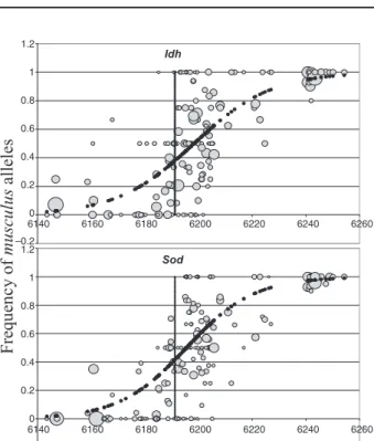
musculus side (this is particularly pronounced for
Es10, Gpd and Pgm). The most pronounced
asymme-try of introgression is seen at the Idh and Sod loci,
whose centre is displaced almost 8 km into the
mus-culus territory as compared with the common centre of
the other loci. For these two loci, no model with a
cen-tral step (around frequency 0.5) fitted the data better
than the simpler sigmoid model (see Fig. 3).
It can also be seen in Figure 2 that there is
consid-erable dispersion of the data points around the model.
This is reflected in the poor precision of the parameter
estimates, given in Table 4 with their two LL support
limits. The variations between loci and the support
limits of the parameters are particularly large for the
left side, with the left barrier parameter absurdly
large for several loci. The parameters defining the
right side of the cline are generally better estimated
and more consistent across loci, but the support limits
still remain rather wide. When the average of the
eight loci with a common centre is used (average
hybrid indices reported in Appendix 1), more reliable
parameter estimates with reasonably narrow support
intervals are obtained (Table
4). The parameters
defining the right and left sides are similar to each
other, and the average cline for these eight loci is
shown graphically in Figure 4. The Y chromosome
data for the same samples (data from Dod et al., 2005,
this issue) are also reported in this figure, showing
that the centre of the allozyme clines corresponds to
the major and abrupt change for this chromosome.
E
STIMATING
SELECTION
PARAMETERS
FROM
CLINE
SHAPES
Given the estimates of cline widths derived above for
the different loci, it is theoretically possible to
esti-mate the migration parameter s using linkage
dise-quilibria between loci in the centre of the hybrid zone.
We estimated the standardized linkage disequilibria
between pairs of loci in each locality for the eight loci
that have coincident centres (Amy, Es1, Es2, Es10,
Gpd, Mpi, Np and Pgm) using the maximum
likeli-hood procedure in the Analyse package. With the
esti-mated cline width for each locus given in Table 4, we
then obtained estimates of the migration parameter.
All pairs of loci are unlinked on the genetic map,
except Es1 and Es2, at 9 cM on chromosome 8, and
Es10 and Np, at 22 cM on chromosome 14, and these
Figure 2. Variations of Mus musculus musculus allele frequencies along the transect across the hybrid zone, for eight
autosomal loci. Shaded circles represent the real data, and the area of the circles is proportional to the effective number
of alleles sampled (after correction for F
ISand F
ST, see text). The filled circles represent the best fit with a common centre
for the eight loci, the position of which is shown by the thin vertical line.
Amy
Es1
Es10
Es2
Gpd
Np
Pgm
Mpi
Geographical coordinate along transect (km)
f
o
yc
ne
u
qe
r
F
sul
ucs
u
m
se
le
ll
a
1.2
1
0.8
0.6
0.4
0.2
0
–0.2
1.2
1
0.8
0.6
0.4
0.2
0
–0.2
1.2
1
0.8
0.6
0.4
0.2
0
–0.2
1.2
1
0.8
0.6
0.4
0.2
0
–0.2
6140
6160
6180
6200
6220
6240
6260
1.2
1
0.8
0.6
0.4
0.2
0
–0.2
6140
6160
6180
6200
6220
6240
6260
1.2
1
0.8
0.6
0.4
0.2
0
–0.2
6140
6160
6180
6200
6220
6240
6260
1.2
1
0.8
0.6
0.4
0.2
0
–0.2
6140
6160
6180
6200
6220
6240
6260
1.2
1
0.8
0.6
0.4
0.2
0
–0.2
6140
6160
6180
6200
6220
6240
6260
6140
6160
6180
6200
6220
6240
6260
6140
6160
6180
6200
6220
6240
6260
6140
6160
6180
6200
6220
6240
6260
values of recombination were used to estimate s. The
results were then averaged over pairs of loci and
local-ities. We chose localities from the centre of the hybrid
zone with more than ten mice in the sample (localities
numbers 102, 106, 120 and 142: Appendix 1). This led
to an average estimate of the migration parameter s of
0.75 km generation
–. We also applied the other
method based on the variance of the hybrid index
(Barton & Gale, 1993) to 145 mice from the 24 most
central populations. The variance of hybrid index was
0.021, and the part due to heterozygosity 0.014. The
excess variance is attributed to linkage
disequilib-1
/
2rium, and with an average cline width of 8.9 km, we
get D = 0.015 and s = 0.77 and 0.63 km generation
–(whether sampling occurred before or after migration,
Barton & Gale, 1993), in good agreement with the
pre-vious estimate.
In order to calculate the intensity of selection
needed to balance dispersal against selection and
recombination, cline shape has to be estimated. To do
this we used the parameters of the average cline for
1/
2Table 4. Maximum likelihood estimates of cline parameters, and their two log-likelihood support limits, for eight loci with
a common centre at position 6191.2
Locus
w
B0/w
q
0B1/w
q
1Amy
20.6 (15.2–26.4)
123.51 (2.27–inf)
0.002 (0.000–0.284)
9.67 (2.74–108.45)
0.037 (0.001–0.157)
Es1
11.0 (2.2–25.2)
0.67 (0.03–5.57)
0.172 (0.010–0.999)
Es10
6.4 (4.9–11.7)
5.15 (1.16–332.67)
0.085 (0.004–0.457)
3.95 (1.81–7.54)
0.016 (0.008–0.055)
Es2
3.8 (1.3–9.2)
14.35 (1.91–123.26)
0.004 (0.000–0.058)
6.50 (1.66–23.25)
0.003 (0.000–0.019)
Gpd
6.3 (3.4–13.0)
2.59 (0.92–27.71)
0.029 (0.002–0.138)
1.09 (0.68–3.05)
0.032 (0.009–0.135)
Mpi
6.2 (2.2–18.9)
2.16 (0.35–9.01)
0.041 (0.004–0.453)
Np
5.9 (3.8–44.6)
0.91 (0.15–inf)
0.045 (0.000–1.000)
2.39 (0.39–7.05)
0.009 (0.002–0.715)
Pgm
6.8 (4.0–9.1)
146.49 (9.98–inf)
0.016 (0.001–0.098)
2.19 (1.91–5.04)
0.035 (0.010–0.061)
Eight loci
8.9 (7.7–12.4)
2.25 (1.09–3.76)
0.072 (0.043–0.163)
2.22 (1.31–3.05)
0.033 (0.023–0.063)
Figure 3. Allele frequency variations along the transect
for two autosomal loci that do not fit the general cline
position and shape of the eight loci in Fig. 2. Symbols are
as in Fig. 2.
Idh
Sod
0
Geographical coordinate along transect (km)
f
o
yc
ne
u
qe
r
F
sul
ucs
u
m
se
le
ll
a
1.2
1
0.8
0.6
0.4
0.2
0
–0.2
6140
6160
6180
6200
6220
6240
6260
1.2
1
0.8
0.6
0.4
0.2
0
–0.2
6140
6160
6180
6200
6220
6240
6260
Figure 4. Allele frequency variations along the transect,
for the average of eight autosomal loci (Amy, Es1, Es2,
Es10, Gpd, Mpi, Np and Pgm), and the Y chromosome (data
from Dod et al., 2005, this issue). Symbols are as in Fig. 2.
Eight allozymes
Y chromosome
Geographical coordinate along transect (km)
musculus
alleles
f
o
yc
ne
u
qe
r
F
1.2
1
0.8
0.6
0.4
0.2
0
–0.2
6140
6160
6180
6200
6220
6240
6260
1.2
1
0.8
0.6
0.4
0.2
0
–0.2
6140
6160
6180
6200
6220
6240
6260
the eight coincident loci. We have seen above that,
individually, most of the clines are asymmetrical, but
that this asymmetry is tempered when the average
introgression over the eight loci is considered. Using
either the right or the left parameters of this cline fit
gives consistent estimates of selection parameters.
The barrier to gene flow on both sides is of the order of
B
~
20 km (2LL support limits 12–33 km on the left
side and 14–28 on the right side), and the height of the
central step in allele frequency equals 0.45. The total
selection acting on the loci studied is estimated as
s* =
0.040–0.059 (eqn
2, with s = 0.63–0.77, see
above). The selection acting on each of the loci causing
the genetic barrier is estimated as s = 0.021–0.030
(eqn 7). The number of loci under selection creating
the central barrier is estimated to be n
~
52–78 by
assuming that the average recombination between the
loci studied and the selected loci is r = 0.5 (eqn 8). This
is thus an overestimate of the number of loci. The
average fitness of hybrid central populations is
esti-mated to be WH = 0.45 (eqn 10). Finally, the selection
acting on the loci under study is estimated using
eqn (5) to be on average of the order of slocus = 0.003–
0.004, or 0.001–0.002 depending on whether the left or
right cline parameters, respectively, are considered.
These low values are in agreement with the
hypothe-sis that was made of weak selection on these loci in
order to apply the approximations needed for the
above parameter estimations.
E
STIMATING
MIGRATION
FROM
MICROSATELLITE
DATA
In order to estimate migration independently of the
cline analyses, we typed some of the populations at six
microsatellite loci and applied various methods of
esti-mation of migration under isolation by distance. We
selected the two sampling years with the largest
sam-ples (1992 and 1998) and analysed the results for each
year separately. Here we are interested in the part of
the genetic differentiation between populations and
individuals that results from migration and drift
alone, so we want to remove the effect of selection in
the hybrid zone. Ideally, this could be done by
analys-ing the residual variation of allele frequencies around
the cline fits for polymorphic, yet diagnostic, markers.
However, most microsatellites tested did not meet
these criteria. We thus chose to study allele frequency
variation among groups of populations more or less
aligned in a direction perpendicular to that of the
cli-nal gradient of the hybrid zone, by restricting the
com-parisons to pairs of populations whose average index
of hybridization for the allozymes differed by less than
10% (Appendix 1).
The 1992 sample consisted of 185 individuals from
14 different localities. For 1998 we used 436 mice from
64 localities. Only 113 mice could be typed for locus
D17Mit14 in the 1992 sample (381 in the 1998
sam-ple), but from 171 to 184 were typed at the five other
loci (from 421 to 436 in 1998). The number of different
alleles found at each locus is indicated in Table 1. The
genotypes of these 621 mice at the six loci are given in
Appendix 3. They include some 1992 data already
reported in Dallas et al. (1995). We retyped a fraction
of the mice from the earlier study to establish the
cor-respondence of allele sizes between the two studies.
For the isolation by distance methods, we not only
restricted the comparisons to pairs of populations with
similar hybridization indexes, as argued above, but
also to pairs not too far from each other, because it is
recommended that pairs be generally separated by no
more than 10s (Rousset, 2000b), and in no case by
more than 20s (Rousset, 2000a). We chose a cut-off at
15 km. By using the FST method on pairs of
popula-tions selected in this way, we derived an estimate of
Ds
2of 3.7 individuals on the 1992 dataset, and of 2.7
individuals for 1998. This method relies on estimates
of population frequencies, and in the regression, data
points are not weighted according to sample sizes, so
these values must be considered with caution. The
and Moran I methods do not have this drawback,
because they are based on comparisons between
indi-viduals, but they appear to be less adapted to the
hab-itat structure of mice, which is fragmented rather
than continuous. They gave consistent estimates of
Ds
2, but showed differences between 1992 (Ds
2= 1.4
and 1.7 for the two methods, respectively) and 1998
(Ds
2= 3.7 and 3.9). The 1998 estimate is presumably
more reliable because many more localities were
sam-pled, so that the range of pairwise distances between
individuals is covered much better.
In order to derive estimates of s, we must now
attempt to estimate the density of mice, which we can
do by using our trapping data. In 1998, the year with
most intense trapping, we underwent a random
pros-pecting of farms, and found that 25% of them had mice.
The average number of mice trapped per farm with
mice was 7.2 (with a large variance, see Table 2).
Because we intensively trapped in all cases, and
stopped the effort only after several unsuccessful
trap-ping nights, we believe this is a reasonable estimate of
the mouse population present. It necessarily provides
a lower limit of the number of mice existing at the time
of trapping, but it includes at least two generations (we
counted both adults and young), and so probably
over-estimates population densities per generation. The
density of farms in the prospected areas was
accu-rately determined by counting them on a map, leading
to an average of 3.1 farms km
-2. This gives an
esti-mated density D of 5.8 mice km
-2. The average Ds
2estimated using the three different isolation by
distance methods ranged from 1.4 to 3.9, which gives
s = 0.51–0.82 km generation
–. If our density
esti-)
a
rmates are really lower limits these estimates of s are
upper limits, but they are compatible with the
esti-mates derived from the cline analyses. With the lowest
value, s = 0.51 km generation
–, we estimate that
the barrier would be created by a larger number
(n = 120) of loci under weaker selection (s = 0.013) than
what is found when estimating migration from linkage
disequilibrium. The highest value of s = 0.82 gives
n = 46 loci with s = 0.035. The results of the two
approaches are comparable, given the numerous
sources of uncertainty associated with these estimates.
DISCUSSION
For eight of the ten allozyme loci studied, the changes
in allele frequencies can be best described by steep
central steps of allele frequency that are coincident
and flanked by smooth tails of introgression on either
side. This indicates the presence of a barrier to gene
flow in the centre of the zone. We assumed that this
barrier is caused by selection against hybrids, creating
a tension zone, and applied the existing theory to
esti-mate the selection and migration parameters shaping
this hybrid zone.
As quantifying migration is essential to infer
selec-tion, we also estimated migration independently from
the cline analysis, using microsatellites and
compar-ing populations of similar positions in the overall
gra-dient of the hybrid zone. The results we obtained using
the different approaches are in good agreement (s =
0.5–0.8 km generation
–). There are few relevant
data in the literature with which to compare this
esti-mate. Many capture–recapture experiments give
dis-cordant results (Lidicker & Patton, 1987), and often
such studies concern small study areas and would
miss long-distance migrants (Baker, 1981; see Pocock,
Hauffe & Searle, 2005, this issue). Myers (1974)
wit-nessed colonization events between grids separated by
92 m. According to Berry & Jakobson (1974) 25% of
the mice on an island mate within 50–100 m from
their birthplace. Carlsen (1993) captured mice in
farms and surrounding fields and reports movements
of up to 130 m. A few studies were able to detect longer
distance migrants. Walkowa, Adamczyk &
Chelkowska (1989) trapped 6.5% of the mice living in
an enclosure in surrounding fields, up to 300 m away.
Cassaing & Croset (1985) recaptured most mice
within 50–480 m in outdoor populations. Auffray et al.
(1990a) report on mice that had covered distances of
up to 700 m, and detected immigration from
popula-tions up to 820 m apart. Berry (1968) describes more
than 30 mice moving 500 m and 14 moving 1500 m.
Migrations over 1000 m are also reported by other
authors (Pearson, 1963; Tomich, 1970). Although most
mice probably reproduce close to their birthplace, they
can apparently easily reach regions several hundreds
1
/
21 2
/
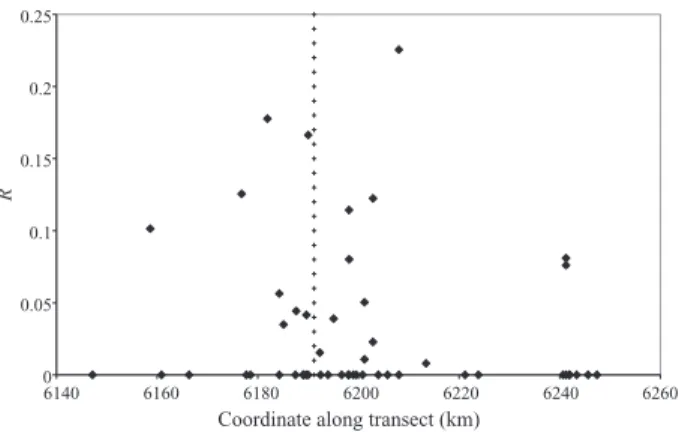
of metres away. In addition, humans can passively
transport them over much longer distances. In
Figure 5 it can be seen that substantial linkage
dis-equilibrium is sometimes found rather far from the
centre of the hybrid zone, and it could be due to such
long-distance migrations. However, we found no
mouse heterozygous at all loci in our dataset, and thus
no F
1mice that could result from such long-distance
migrations. Potential first-generation backcrosses,
heterozygous at half of their loci, were rare: only one
was found on the domesticus side of the zone (among
151 mice from localities with a coordinate lower than
6182 and with data available at eight loci or more). Six
such mice were found on the musculus side (among
359 mice from localities with a coordinate above 6200),
but only from the localities closest to the central step
of the hybrid zone (coordinates from 6200–6205).
The average barrier to gene flow appears relatively
moderate (20 km) compared with migration (0.5–
0.8 km generation
–), but varies considerably
between loci in our estimates, as well as the level of
introgression and degree of asymmetry. Two of the loci
we studied (Idh and Sod) did not show the typical
cen-tral step, but rather wide clines with extensive
intro-gression into musculus, which could be an indication
that they have escaped the central barrier. The delay
to introgression of neutral alleles across such a barrier
is expected to be of the order of 500–1600 generations
(B
2/s
2; Barton & Hewitt, 1985, and references
therein). There are presumably two reproduction
peri-ods per year, one indoors in autumn that we observed
during our trapping campaigns and a second one in
spring, mostly in the fields. This would, however,
rep-resent only one generation a year in terms of
migra-tion. According to what is believed about the patterns
of expansion of these subspecies (reviewed in Boursot
1