HAL Id: ird-01920130
https://hal.ird.fr/ird-01920130
Submitted on 11 Jul 2019
HAL is a multi-disciplinary open access
archive for the deposit and dissemination of sci-entific research documents, whether they are pub-lished or not. The documents may come from teaching and research institutions in France or abroad, or from public or private research centers.
L’archive ouverte pluridisciplinaire HAL, est destinée au dépôt et à la diffusion de documents scientifiques de niveau recherche, publiés ou non, émanant des établissements d’enseignement et de recherche français ou étrangers, des laboratoires publics ou privés.
Multidimensional scaling with very large datasets
Emmanuel Paradis
To cite this version:
Emmanuel Paradis. Multidimensional scaling with very large datasets. Journal of Computational and Graphical Statistics, Taylor & Francis, 2018, pp.1 - 5. �10.1080/10618600.2018.1470001�. �ird-01920130�
Multidimensional scaling with very large
data sets
Emmanuel Paradis
April 6, 2018
ISEM, IRD, Univ. Montpellier, CNRS, EPHE, Montpellier, France
E-mail: [email protected]
Abstract: Multidimensional scaling has a wide range of applications when observa-tions are not continuous but it is possible to define a distance (or dissimilarity) among them. However, standard implementations are limited when analyzing very large data sets
3
because they rely on eigendecomposition of the full distance matrix and require very long computing times and large quantities of memory. Here, a new approach is developed based on projection of the observations in a space defined by a subset of the full data set. The
6
method is easily implemented. A simulation study showed that its performance are satis-factory in different situations and can be run in a short time when the standard method takes a very long time or cannot be run because of memory requirements.
9
1
Introduction
Multidimensional scaling (MDS) aims to find a set of coordinates in one or several
dimen-12
sions, so that the distances derived from these coordinates are the closest possible to the observed distances. By contrast to principal component analysis (PCA), MDS (also called principal coordinates analysis, PCoA) does not require a set of original coordinates. This
15
is a very attractive feature since a distance can naturally be defined for many types of data whereas these data do not easily define a system of coordinates (e.g., DNA sequences, graphs, psychological profiles). A search of the string “multidimensional scaling” in the
18
Web of Science returned 7313 hits (accessed 2017-07-31) with the highest proportions of publications in the fields of environmental sciences & ecology (15.9%), psychology (14.9%), and computer science (14.7%).
21
MDS is basically done through a decomposition of the symmetric distance matrix among observations. This matrix as thus has many rows and columns than there are observations, and its decomposition with standard eigenvalue analysis algorithm can be a limiting factor
24
when this number is large. In a context where many scientific fields collect large amounts of data, this is clearly a severe limitation. Some examples include genomic analyses from high throughput sequencing technologies which typically handle millions of DNA sequences,
27
or environmental data from high-resolution remote sensing which represent variables for millions of localities on the Earth’s surface.
In this paper, I present an approach to avoid the limitations of the standard procedure
30
of MDS. In the next section, I present the different computational procedures considered in this paper. Section 3 reports the results from a simulation study. The last section discusses these results and presents some perspectives.
33
2
Computational procedures
Section 2.1 below describes the standard MDS procedure; Section 2.2 explains how this procedure can be extended with random matrix algorithms. Sections 2.3 and 2.4 introduce
36
2.1
Standard multidimensional scaling
Let us denote n the number of observations, and ∆ the n × n symmetric matrix of distances
39
with δij (= δji) being the distance between observations i and j. MDS proceeds by doing
an eigendecomposition of the doubly-centred distance matrix:
−1 2J ∆
2J, (1)
with J = I − n111T. The matrix of coordinates Z are calculated with:
42
Z = V Λ1/2,
where V is an n × k matrix with the first k eigenvectors extracted from (1), and Λ is a diagonal k × k matrix with the first k eigenvalues (λ1, . . . , λk). Z has therefore n rows and
k columns. The value of k is the number of dimensions of the projected space and is chosen
45
by the investigator, usually depending on the values of λ.
This procedure involves manipulating matrices with n2elements which is very expensive in terms of memory requirements and computing times when n is large.
48
2.2
Eigendecomposition with random matrices
Halko et al. (2011) presented several algorithms to decompose very large matrices. These algorithms are based on random matrices and can extract several eigenvalues in a few
51
seconds while it would take several hours to perform the same operation with classical eigendecomposition. The eigenvalues are extracted sequentially, by contrast to the standard MDS where all eigenvalues are calculated at once, even if only some of them are used to
54
calculate the coordinates in Z. Therefore, random matrix algorithms make possible to decompose very large matrices which could not be analyzed with the standard approach because of memory limitations. Here, we use the implementation from Abraham & Inouye
57
and their package flashpcaR (Abraham & Inouye 2014).
2.3
1-D projection
The principle of this method is quite simple. In a first step, m observations are selected
60
coordinate of the ith observation (i = 1, . . . , m). In a second step, for each observation j not among the m selected in step 1, the coordinate zj is found by minimizing:
63 f = m X i=1 (δij − dij)2, (2)
with dij = |zi− zj|. We may write the latter as:
dij = γi(zi− zj) γi = +1 zj < zi −1 zj ≥ zi,
A simple algebraic development leads to:
f = m X i=1 δ2ij − 2 m X i=1 (δijγizi− δijγizj) + m X i=1 zi2− 2zj m X i=1 zi+ mzj2.
We can now write the partial derivative of f with respect to zj:
66 ∂f ∂zj = 2 m X i=1 δijγi− 2 m X i=1 zi+ 2mzj. Writing ¯z = m1 Pm
i=1zi and solving the last expression leads us to find the value zj that
minimizes f : 1 m m X i=1 δijγi− ¯z + zj = 0.
Given that there are only m distances δij to calculate, and that ¯z is calculated only once,
69
this equation can be solved numerically relatively easily. During the first step, m(m − 1)/2 distances are computed for the classical MDS. Thus, the memory requirements of this method are very small. Overall, instead of calculating n(n − 1)/2 distances for a full MDS,
72
this method requires to calculate nm − m(m + 1)/2 distances.
The choice of the m observations is important for this projection procedure to work as best as possible. They should represent as much as possible the distribution of the n
75
observations. This is not straightforward since the projection of these n points in the MDS space is not known a priori. In order to solve this issue, the following algorithm selects m observations so their distances are representative of the whole set of distances:
78
1. Select one observation i at random among the n ones; store i.
3. Find j0 so that δij0 is max of the distances calculated at step 2; store j0. 81
4. Compute the distances δj0j with j among the values not yet stored.
5. Select i so that δj0i is median of the distances calculated at step 4; store i.
6. Repeat steps 2–5 until m values are stored.
84
This algorithm may be used whatever the number of dimensions k. There could be some variants of this algorithm: for instance, instead of the median in step 5, one could select a random distance δj0i so that the observations will be represented in proportion of their 87
relative frequencies (somehow similar to an MCMC procedure).
2.4
Higher dimension projection
The method developed above can be generalized to more than one dimension in a
straight-90
forward way. The distances dij in (2) would then be calculated as Euclidean distances in
the projection space:
dij = v u u t k X l=1 (zil− zjl)2
In this case, the partial derivatives can be derived but are too complicated to be useful,
93
so it is more efficient to rely on a standard minimization procedure to minimize (2). Two procedures were tested here: the classical BFGS method (Broyden 1970, Fletcher 1970, Goldfarb 1970, Shanno 1970) and the PORT routine (Gay 1990).
96
3
Simulation study
A simulation study was conducted to answer two questions: What are the computing times of the different procedures described above? and, What are their respective accuracy? The
99
data were simulated from a standard normal distribution with one or two dimensions and with different samples sizes n (1000, 5000, 10,000, and 50,000). The projection procedures were performed with m = 100 points chosen randomly. To assess the accuracy of the results,
102
two quantities were calculated. First, the classical stress was calculated with Kruskal’s formula (Kruskal 1964):
S = v u u u u u u u t n X i,j (δij − dij)2 n X i,j δij2 .
This quantity varies between 0 (complete mismatch of the distances) and 1 (perfect match).
105
Second, a measure of the accuracy of the inferred distances was calculated with:
S0 = n X i,j (δij − dij)2 δij .
This second quantity is similar to Sammon’s criterion (Sammon 1969) and gives more emphasis on the precision of each distance whereas Kruskal’s stress puts emphasis on the
108
overall precision of the distances. In addition, in order to assess whether the observed results were better than simply randomly positioning the points in the MDS space, both quantities were calculated after randomizing the simulated data.
111
The simulations were run with k = 1 and k = 2. In the second case, the two variables were either independent or with a correlation of 0.7. Additionally, skewed distributions were generated with k = 1 in order to simulate aggregation of points. Two cases were
114
considered: an exponential distribution with rate equal to one, and a mixture of two normal distributions with means −5 and 5 and proportions 0.9 and 0.1, respectively. In these two cases, the analyses were performed with m = 100 observations selected randomly
117
like previously, and using the algorithm described above. All simulations were replicated 100 times and run on a computer equipped with a duo-core, 2.1 GHz processor and 16 GB of RAM, and running Ubuntu 16.04. All computations were implemented in R version 3.4.1
120
(R Core Team 2017); the code is available as supplementary material with this article.
3.1
1-D MDS
With a moderate sample size n = 1000, the three methods considered here completed in less
123
than one second (Table 1). However, with n = 10,000, the standard MDS took almost dour minutes while the same procedure with a random decomposition took slightly more than eleven seconds, and the projection method took less than one second. Most importantly,
126
the computing times of the latter appeared to be linearly related with n whereas the two others seemed to run proportionally to n3 for the standard MDS, or to n2 for the random
Table 1: Computing times of different 1-D MDS methods (in seconds). Method n 1000 5000 10,000 50,000 Standard MDS 0.33 26.47 220.94 – Random eigendecomposition 0.09 1.09 11.66 – 1-D Projection (m = 100) 0.11 0.41 0.79 3.91
Table 2: Stress (S) from different 1-D MDS methods.
Method n 1000 5000 10,000 50,000 Standard MDS 1.6 × 10⁻¹⁵ 2.7 × 10⁻¹⁵ 3.6 × 10⁻¹⁵ – Random eigendecomposition 1.7 × 10⁻² 7.6 × 10⁻³ 6.9 × 10⁻³ – 1-D Projection (m = 100) 9.1 × 10⁻⁶ 9.5 × 10⁻⁶ 9.3 × 10⁻⁶ 9.7 × 10⁻⁶ “random” 9.5 × 10⁻¹ 8.5 × 10⁻¹ 8.5 × 10⁻¹ 8.5 × 10⁻¹
decomposition. The computing time of the two decomposition-based methods was not
129
assessed with n = 50,000.
Unsurprisingly, the standard MDS performed the best considering either the stress S (Table 2) or the accuracy of the inferred distances S0 (Table 3). The projection method
132
performed the second best and better than the random decomposition method. All methods performed better than randomly projecting the points.
Table 3: Accuracy of inferred distances (S0) from different 1-D MDS methods.
Method n 1000 5000 10,000 50,000 Standard MDS 6.7 × 10⁻²⁴ 1.3 × 10⁻²¹ 9.2 × 10⁻²¹ – Random eigendecomposition 2.8 × 10² 1.4 × 10³ 3.7 × 10³ – 1-D Projection (m = 100) 3.8 × 10⁻⁴ 9.7 × 10⁻³ 3.8 × 10⁻² 9.8 × 10⁻¹ “random” 8.7 × 10⁶ 4.3 × 10⁸ 1.1 × 10⁹ 3.4 × 10¹⁰
Table 4: Computing times of different 2-D MDS methods (in seconds). Method n 1000 5000 10,000 50,000 Standard MDS 0.32 26.32 221.60 – Random eigendecomposition 0.07 1.13 12.35 – 2-D Projection (m = 100) with BFGS 0.59 3.01 6.06 33.58 with PORT 0.33 1.58 3.20 17.62
Table 5: Stress (S) from different 2-D MDS methods.
Method n 1000 5000 10,000 50,000 Standard MDS 1.6 × 10⁻¹⁵ 2.4 × 10⁻¹⁵ 4.5 × 10⁻¹⁵ – Random eigendecomposition 2.0 × 10⁻² 9.2 × 10⁻³ 6.1 × 10⁻³ – 2-D Projection (m = 100) with BFGS 5.4 × 10⁻⁸ 5.7 × 10⁻⁸ 5.7 × 10⁻⁸ 5.7 × 10⁻⁸ with PORT 4.5 × 10⁻¹⁰ 4.9 × 10⁻¹⁰ 4.5 × 10⁻¹⁰ 4.7 × 10⁻¹⁰ “random” 6.6 × 10⁻¹ 6.5 × 10⁻¹ 6.5 × 10⁻¹ 6.5 × 10⁻¹
3.2
2-D MDS
135The two methods based on matrix decomposition showed similar computing times than in one dimension (Table 4). On the other hand, the projection method was slower but its computing times still scaled proportionally to n. The PORT-based projection method was
138
almost twice faster than the BFGS-based one.
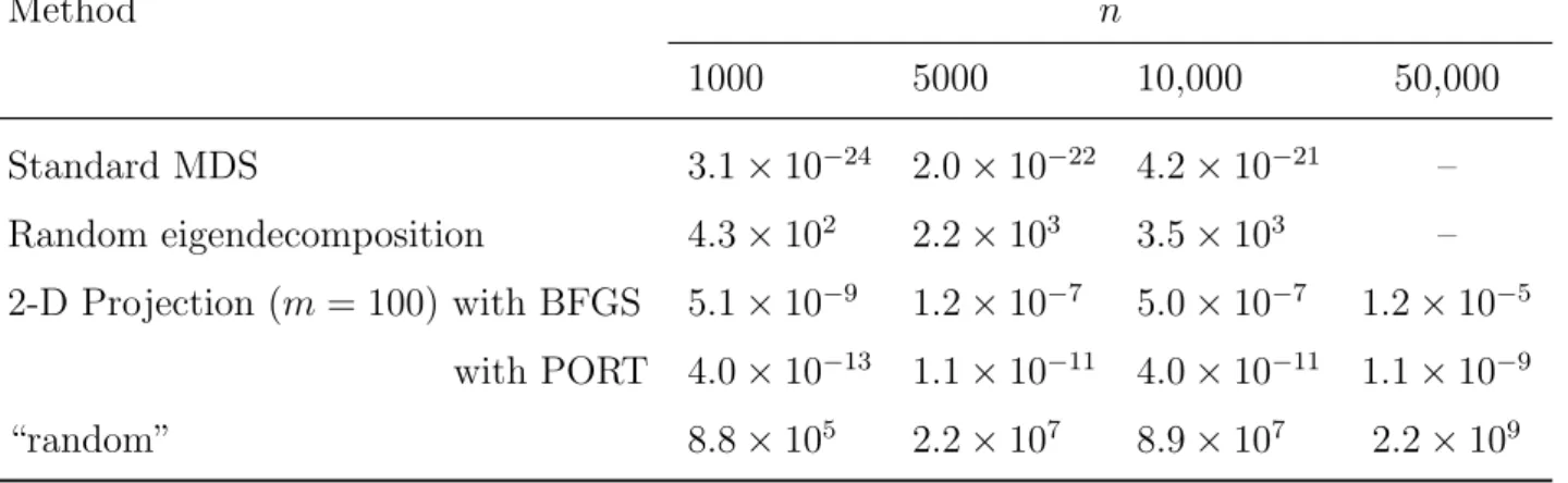
With two independent variables, the accuracy of the projection methods were less than the standard MDS but these methods appeared still accurate (Tables 5 and 6). The
PORT-141
based variant was more accurate than the BFGS-based one. By constrast, the random decomposition method performed poorly. When the two variables were correlated, the performance of the standard MDS and the projection methods were similar to the previous
144
situation; however, the performance of the random decomposition method deteriorated considerably and were only slightly better than randomly positioning the data (Tables 7 and 8).
Table 6: Accuracy of inferred distances (S0) from different 2-D MDS methods. Method n 1000 5000 10,000 50,000 Standard MDS 3.1 × 10⁻²⁴ 2.0 × 10⁻²² 4.2 × 10⁻²¹ – Random eigendecomposition 4.3 × 10² 2.2 × 10³ 3.5 × 10³ – 2-D Projection (m = 100) with BFGS 5.1 × 10⁻⁹ 1.2 × 10⁻⁷ 5.0 × 10⁻⁷ 1.2 × 10⁻⁵ with PORT 4.0 × 10⁻¹³ 1.1 × 10⁻¹¹ 4.0 × 10⁻¹¹ 1.1 × 10⁻⁹ “random” 8.8 × 10⁵ 2.2 × 10⁷ 8.9 × 10⁷ 2.2 × 10⁹
Table 7: Stress (S) from different 2-D MDS methods with correlated variables.
Method n 1000 5000 10,000 50,000 Standard MDS 1.4 × 10⁻¹⁵ 2.2 × 10⁻¹⁵ 2.7 × 10⁻¹⁵ – Random eigendecomposition 5.5 × 10⁻¹ 5.5 × 10⁻¹ 5.5 × 10⁻¹ – 2-D Projection (m = 100) with BFGS 5.4 × 10⁻⁸ 5.9 × 10⁻⁸ 5.5 × 10⁻⁸ 6.0 × 10⁻⁸ with PORT 1.9 × 10⁻¹⁰ 2.1 × 10⁻¹⁰ 2.0 × 10⁻¹⁰ 2.1 × 10⁻¹⁰ “random” 7.4 × 10⁻¹ 7.4 × 10⁻¹ 7.5 × 10⁻¹ 7.4 × 10⁻¹
Table 8: Accuracy of inferred distances (S0) from different 2-D MDS methods with corre-lated variables. Method n 1000 5000 10,000 50,000 Standard MDS 3.3 × 10⁻²⁴ 2.7 × 10⁻²² 1.6 × 10⁻²¹ – Random eigendecomposition 2.9 × 10⁵ 7.0 × 10⁶ 2.9 × 10⁷ – 2-D Projection (m = 100) with BFGS 8.9 × 10⁻⁹ 2.5 × 10⁻⁷ 7.7 × 10⁻⁷ 2.3 × 10⁻⁵ with PORT 1.1 × 10⁻¹⁴ 2.8 × 10⁻¹² 1.0 × 10⁻¹¹ 2.8 × 10⁻¹⁰ “random” 1.5 × 10⁶ 3.7 × 10⁷ 1.5 × 10⁸ 3.7 × 10⁹
Table 9: Results of simulations with an exponential variable. CT: computing times (in seconds). Sampling m = 100 observations with the algorithm presented in this paper (A) or uniformly (U). n Sampling 1000 5000 10,000 50,000 CT A 0.06 0.35 0.72 3.86 U 0.06 0.36 0.73 3.93 S A 8.3 × 10⁻⁶ 8.6 × 10⁻⁶ 8.9 × 10⁻⁶ 8.6 × 10⁻⁶ U 1.0 × 10⁻⁵ 1.1 × 10⁻⁵ 1.1 × 10⁻⁵ 1.1 × 10⁻⁵ S0 A 5.6 × 10⁻⁴ 1.4 × 10⁻² 6.0 × 10⁻² 1.33 U 8.7 × 10⁻⁴ 2.1 × 10⁻² 8.3 × 10⁻² 2.16
3.3
Skewed Distributions
For the two methods based on matrix decomposition, the results with the skewed distri-butions were very similar to the previous ones, and are thus not reported here. For the
150
1-D projection method, the analyses were performed with a uniform random sample and using the algorithm described above. Both algorithms resulted in similar computing times; however, the uniform sampling resulted in decreased accuracy while the above algorithm
153
yielded performance comparable to the previous ones with non-aggregated data. This difference in accuracy was small for the data simulated from an exponential distribution (Table 9) whereas it was important for the mixture of normal variables where the skewness
156
of the data was much more pronounced (Table 10).
4
Discussion
This article presents a method to perform MDS on very large data sets in short times and
159
with small memory requirements. The objective of the present study was to develop a method easily implemented and generally applicable. One initial motivation was to avoid the need to perform a matrix decomposition of the full distance matrix as used in standard
162
MDS.
Two approaches were considered in this study: the first one used matrix decomposition algorithms based on random matrices, and the second one used a projection algorithm
Table 10: Results of simulations with a mixture of two random variables. CT: computing times (in seconds). Sampling m = 100 observations with the algorithm presented in this paper (A) or uniformly (U).
n Sampling 1000 5000 10,000 50,000 CT A 0.06 0.35 0.70 3.68 U 0.07 0.36 0.73 3.85 S A 2.9 × 10⁻⁶ 3.0 × 10⁻⁶ 3.0 × 10⁻⁶ 2.9 × 10⁻⁶ U 4.1 × 10⁻² 4.3 × 10⁻² 4.2 × 10⁻² 4.2 × 10⁻² S0 A 3.0 × 10⁻⁴ 7.4 × 10⁻³ 2.9 × 10⁻² 7.3 × 10⁻¹ U 9.8 × 10³ 2.1 × 10⁵ 7.8 × 10⁵ 1.8 × 10⁷
based on a subset of points. The first approach did not appear as a viable solution to handle large data sets: it was too slow for sample sizes larger than 10,000 and was very inacurrate in some situations. This method performed poorly with correlated variables,
168
which was an unexpected result. It is unclear whether this a pathological specific case or a more general problem with random decomposition of distance matrices. Further tests will be needed to clarify this point.
171
One issue not treated in depth in the present work is how to select the number of dimen-sions (k). In standard MDS, this value is selected depending on the eigenvalues extracted from the decomposition of the distance matrix. Typically, in practical applications of MDS
174
two dimensions are selected in order to provide an interpretable graphical display. With the projection method proposed in this paper, since the number of dimensions determines the algorithm used, this number may be selected with respect to the eigenvalues of the
177
standard MDS done on the subset of size m.
Another issue not explored here is the choice of the size of the subset (m). It was found that a value m = 100 is appropriate in the situations considered here: it makes possible
180
to perform the projection easily since a larger value would make this procedure slower and more complicated. An interesting result was the good performance of the selection algorithm presented in this paper, particularly if the data were aggregated. This also
183
deserves further study.
researchers need to analyze increasingly larger data sets, such as in ecological habitat
186
modeling based on remote sensing (Hansen et al. 2008) or in genomic analysis (Erlich 2015). It will thus be interesting to see how the present method behaves and performs in practical applications.
189
Acknowledgments
I am grateful to an anonymous reviewer for helpful comments on a previous version of this paper. This is publication ISEM 2017-201.
192
SUPPLEMENTARY MATERIAL
functions MDS.R: R functions used to perform the methods described in this paper. sim.R: R functions used to perform the simulations reported in this paper.
195
References
Abraham, G. & Inouye, M. (2014), ‘Fast principal component analysis of large-scale genome-wide data’, PLoS ONE 9(4), e93766.
198
Broyden, C. G. (1970), ‘The convergence of a class of double-rank minimization algorithms 1. General considerations’, Journal of the Institute of Mathematics and its Applications 6(1), 76–90.
201
Erlich, Y. (2015), ‘A vision for ubiquitous sequencing’, Genome Research 25(10), 1411– 1416.
Fletcher, R. (1970), ‘A new approach to variable metric algorithms’, Computer Journal
204
13(3), 317–322.
Gay, D. M. (1990), Usage summary for selected optimization routines, Technical Report Computing Science Technical Report No. 153, AT&T Bell Laboratories, Murray Hill, NJ
207
07974, USA.
URL: http://netlib.bell-labs.com/netlib/port/
Goldfarb, D. (1970), ‘A family of variable metric updates derived by variational means’,
210
Mathematics of Computation 24, 23–26.
probabilistic algorithms for constructing approximate matrix decompositions’, SIAM
Re-213
view 53(2), 217–288.
Hansen, M. C., Stehman, S. V., Potapov, P. V., Loveland, T. R., Townshend, J. R. G., DeFries, R. S., Pittman, K. W., Arunarwati, B., Stolle, F., Steininger, M. K., Carroll,
216
M. & DiMiceli, C. (2008), ‘Humid tropical forest clearing from 2000 to 2005 quantified by using multitemporal and multiresolution remotely sensed data’, Proceedings of the National Academy of Sciences USA 105(27), 9439–9444.
219
Kruskal, J. B. (1964), ‘Multidimensional scaling by optimizing goodness of fit to a nonmetric hypothesis’, Psychometrika 29(1), 1–27.
R Core Team (2017), R: A Language and Environment for Statistical Computing, R
Foun-222
dation for Statistical Computing, Vienna, Austria. URL: http://www.R-project.org
Sammon, Jr, J. W. (1969), ‘A nonlinear mapping for data structure analysis’, IEEE
Trans-225
actions on Computers C-18(5), 401–409.
Shanno, D. F. (1970), ‘Conditioning of quasi-Newton methods for function minimization’, Mathematics of Computation 24, 647–656.