Adaptive array processing for multiple microphone hearing aids

Adaptive Array Processing for Multiple Microphone

Hearing Aids

RLE Technical Report No. 541

February 1989

Patrick M. Peterson

Research Laboratory of Electronics Massachusetts Institute of Technology

Adaptive Array Processing for Multiple Microphone

Hearing Aids

RLE Technical Report No. 541

February 1989

Patrick M. Peterson

Research Laboratory of Electronics Massachusetts Institute of Technology

Cambridge, MA 02139 USA

This work has been supported in part by a grant from the National Institute of Neurological and Communicative Disorders and Stroke of the National Institutes of Health (Grant R01-NS21322).

Adaptive Array Processing for

Multiple Microphone Hearing Aids

by

Patrick M. Peterson

Submitted to the Department of Electrical Engineering and Computer Science on February 2, 1989 in partial fulfillment of the

requirements for the degree of Doctor of Science

Abstract

Hearing-aid users often have difficulty functioning in acoustic environments with many sound sources and/or substantial reverberation. It may be possible to improve hearing aids (and other sensory aids, such as cochlear implants or tactile aids for the deaf) by using multiple microphones to distinguish between spatially-separate sources of sound in a room. This thesis examines adaptive beamforming as one method for combining the signals from an array of head-mounted microphones to form one signal in which a particular sound source is emphasized relative to all other sources.

In theoretical work, bounds on the performance of adaptive beamformers are calculated for head-sized line arrays in stationary, anechoic environments with isotropic and multiple-discrete-source interference. Substantial performance gains relative to a single microphone or to conventional, non-adaptive beamforming are possible, depending on the interference, allowable sensitivity to sensor noise, array orientation, and number of microphones. Endfire orientations often outperform broadside orientations and using more that about 5 microphones in a line array does not improve performance.

In experimental work, the intelligibility of target speech is measured for a two-microphone beamformer operating in simulated environments with one interference source and different amounts of reverberation. Compared to a single microphone, beamforming improves the effective target-to-interference ratio by 30, 14, and 0 dB in anechoic, moderate, and severe reverberation. In no case does beamforming lead to worse performance than human binaural listening.

Thesis Supervisor: Nathaniel Durlach Title: Senior Scientist

ACKNOWLEDGEMENTS

Although I must accept full responsibility for the contents of this thesis, it is only part of a larger "Multi-Mike" collaboration among members of the MIT Sensory Communication Group, in particular, Pat Zurek, Bill Rabinowitz, Nat Durlach, Roel Hammerschlag, Su-Min Wei, and Julie Greenberg. I use the first-person plural throughout the thesis to acknowledge the innumerable contributions of these coworkers. Nat Durlach supervised the thesis and William Siebert, Bruce Musicus, and Arthur Baggeroer served as readers. Most of the work was supported under grant R01-NS21322 from the National Institute of Neurological and Communicative Disorders and Stroke. On a personal level, I would also like to acknowledge the help and encouragement of my family and all my friends in the Sensory Communication Group and elsewhere (You know who you are!).

Contents

Abstract 2

1 Introduction

1.1 A Deficiency in Monaural Hearing-Aids ... 1.2 A Strategy for Improvement ...

2 Background

2.1 Human Speech Reception in Rooms ... 2.2 Present Multi-microphone Aids ... 2.3 Multi-microphone Arrays ... 2.3.1 Received Signals. 2.3.2 Signal Processing . 2.3.3 Response Measures . 6 6 7 11 11 14 15 16 24 28

3 Optimum Array Processing 37

3.1 Frequency-Domain Optimum Processors ... 37

3.1.1 Maximum A Posteriori Probability ... 40

3.1.2 Minimum Mean Squared Error ... 42

3.1.3 Maximum Signal-to-Noise Ratio ... ... 43

3.1.4 Maximum-Likelihood . . . ... 44

3.1.5 Minimum-Variance Unbiased ... 46

3.1.6 Summary ... 47

3.2 Time-Domain Optimum Processors . ... 49

3.2.1 Minimum Mean-Square Error . . . ... 50

3.2.2 Minimum Variance Unbiased ... 51

3.2.3 Summary ... 53 3.3 Comparison of Frequency- and Time-Domain Processing . 54

4

_~~~~~~~~~~~~~~~~~~~~~~~~~~~~~~~~~~~~~~~~~~~~~~~~~~~~~~--4 Optimum Performance

4.1 Uncorrelated Noise ... 4.2 Isotropic Noise ...

4.2.1 Fundamental Performance Limits ...

4.2.2 Performance Limits for Hearing-Aid Arrays . . 4.3 Directional Noise ...

4.3.1 Performance against One Directional Jammer 4.3.2 Performance against Multiple Jammers 4.4 Directional Noise in Reverberation ... 4.5 Head Shadow and Other Array Configurations

5 Adaptive Beamforming 5.1 Frost Beamformer. 5.2 Griffiths-Jim Beamformer. 5.3 Other Methods. 6 Experimental Evaluation 6.1 Methods.

6.1.1 Microphone Array Processing .... 6.1.2 Simulated Reverberant Environments 6.1.3 Intelligibility Tests. 6.2 Results . ... 6.2.1 Intelligibility Measurements. 6.2.2 Response Measurements. 56 58 .. . . . 60 61 63 71 73 80 88 89 93 COI . . . ... 95 .. .. ... . .. . .. . .98 99 . . . .99 . . . 99 ... 100 ... . . . 102 ... . . . 104 ... . . . 104 ... . . . 105 109

7 Summary and Discussion

A Useful Matrix Identities 114

B Equivalence of Two Optimum Weights

. . . . . . . . . . . . . . . . . . . . . . . . . . . . 115

Chapter 1

Introduction

1.1

A Deficiency in Monaural Hearing-Aids

Hearing-impaired listeners using monaural hearing aids often have difficulty under-standing speech in noisy and/or reverberant environments (Gelfand and Hochberg, 1976; Nabelek, 1982). In these situations, the fact that normal listeners have less difficulty, due to a phenomenon of two-eared listening known as the "cocktail-party effect" (Koenig, 1950; Kock, 1950; Moncur and Dirks, 1967; MacKeith and Coles, 1971; Plomp, 1976), indicates that impaired listeners might do better with aids on both ears (Hirsh, 1950). Unfortunately, this strategy doesn't always work, possibly because hearing impairments can degrade binaural as well as monaural abilities (Jerger and Dirks, 1961; Markides, 1977; Siegenthaler, 1979). Furthermore, it is often impossible to provide binaural aid, as in the case of a person with no hearing at all in one ear, or in the case of persons with tactile aids or cochlear implants, where sensory limitations, cost, or risk preclude binaural application. All of these effectively-monaural listeners find themselves at a disadvantage in understanding speech in poor acoustic environments. A single output hearing aid that enhanced "desired" signals in such environments would be quite useful to these impaired listeners.

Such an aid could be built with a single microphone input if a method were available for recovering a desired speech signal from a composite signal containing interfering speech or noise. Although much research has been devoted to such single-channel speech enhancement systems (Frazier, Samsam, Braida and Oppenheim, 1976; Boll, 1979; Lim and Oppenheim, 1979), no system has been found effective in increasing speech intelligibility (Lim, 1983) 1. Fundamentally, single-microphone 1Recent adaptive systems proposed for single-channel hearing aids apply adaptive linear bandpass

6

-systems cannot provide the direction-of-arrival information which two-eared listen-ers use to discriminate among multiple talklisten-ers in noisy environments (Dirks and Moncur, 1967; Dirks and Wilson, 1969; Blauert, 1983).

1.2

A Strategy for Improvement

This thesis will explore the strategy of using multiple microphones and adaptive combination methods to construct adaptive multiple-microphone monaural aids (AMMAs). For spatially-separated sound sources in rooms, multiple microphones in a spatially-extended array will often receive signals with intermicrophone differences that can be exploited to enhance a desired signal for monaural presentation. The effectiveness of this "spatial-diversity" strategy is indicated by the fact that it is employed by almost all natural sensory systems. In human binaural hearing, the previously mentioned cocktail-party effect is among the advantages afforded by spatial diversity (Durlach and Colburn, 1978).

To truly duplicate the abilities of the normal binaural hearing system, a monau-ral aid should enable the listener to concentrate on a selected source while mon-itoring, more or less independently, sources from other spatial positions (Durlach and Colburn, 1978). In principle, these abilities could be provided by first resolving spatially-separate signal sources and then appropriately coding the separated infor-mation into one monaural signal. While other researchers (Corbett, 1986; Durlach, Corbett, McConnell, et al., 1987) investigate the coding problem, this thesis will concentrate on the signal separation problem. The immediate goal is a processor that enhances a signal from one particular direction (straight-ahead, for example). filtering to the composite signal by either modifying the relative levels of a few different frequency bands (Graupe, Grosspietsch and Basseas, 1987), or by modifying the cutoff-frequency of a high-pass filter (Ono, Kanzaki and Mizoi, 1983). As we will discuss in more detail later, speech intelligibility depends primarily on speech-to-noise ratio in third-octave-wide bands, with slight degradations due to "masking" when noise in one band is much louder than speech in an adjacent band. Since the proposed adaptive filtering systems cannot alter the within-band speech-to-noise ratio, we would expect no intelligibility improvement except in the case of noises with pronounced spectral peaks. Careful evaluations of these systems (Van Tassell, Larsen and Fabry, 1988; Neuman and Schwander, 1987) confirm our expectations about intelligibility. Of course, hearing-aid users also consider factors beyond intelligibility, such as comfort, that may well be improved with adaptive filtering.

CHAPTER 1. INTRODUCTION

Many of these processors, each enhancing signals from different directions and all operating simultaneously, would form a complete signal separation system for the ultimate AMMA. However, even a single, straight-ahead directional processor could provide useful monaural aid in many difficult listening situations.

The existence of the cocktail party effect indicates that information from multi-ple, spatially-separated acoustic receivers can increase a selected source's intelligi-bility. Unfortunately, we do not understand human binaural processing well enough to duplicate its methods of enhancing desired speech signals. Certain phenomena, such as the precedence effect (Zurek, 1980), indicate that this enhancement involves non-linear processing, which can be difficult to analyze and may not be easy to synthesize.

Linear processing, on the other hand, which simply weights and combines signals from a receiver array, can be easily synthesized to optimize a mathematical perfor-mance criterion, such as signal-to-noise ratio (SNR). Although linear processing may ultimately prove inferior to some as-yet-unknown non-linear scheme, and although improving SNR does not necessarily improve intelligibility (Lim and Oppenheim, 1979), the existence of a well-defined mathematical framework has encouraged research and generated substantial insight into linear array processing techniques. Techniques based on antenna theory (Elliott, 1981) can be used to design fixed weightings that have unity gain in a desired direction with minimum average gain in all other directions. However, if we restrict microphone placement (for cosmetic or practical reasons) t locations on a human head, then the array size will be small relative to acoustic wavelengths and overall improvements will be limited. On the other hand, adaptive techniques developed in radar, sonar, and geophysics can provide much better performance by modifying array weights in response to the actual interference environment (Monzingo and Miller, 1980). The existence of a substantial literature and the success of adaptive arrays in other applications make them an attractive approach to developing AMMAs.

To date, only a few attempts have been made to apply adaptive array techniques to the hearing aid problem (Christiansen, Chabries and Lynn, 1982; Brey and Robinette, 1982; Foss, 1984). These attempts have generally proven inconclusive,

---··11·1--·11)·11111(_·__ls ----· I _I __ _I_

either because they used unrealistic microphone placements (i.e., near the sound sources) or because they used real-time hardware that severely limited performance. In no case has the potential problem of reverberation been addressed and there has been no effort to compare alternative methods.

This thesis will focus on determining the applicability of adaptive array pro-cessing methods to hearing aids and to the signal separation problem in particular. We will not look at fixed array weighting systems or non-linear processing schemes, although other researchers should not overlook these alternate approaches. Fur-thermore, we will not directly address the issue of practicality. Our primary goal is to determine the potential benefits of adaptive array processing in the hearing aid environment, independent of the practicality of realizing these benefits with current technology.

We will determine the potential of array processing both theoretically and ex-perimentally. Theoretical limits on signal-to-noise ratio (SNR) improvement can be calculated for particular environments and array geometries independent of the processing algorithm. Experimentally, specific algorithms can be implemented and actual improvements in SNR and intelligibility can then be measured and related to the theoretical limits.

The effects of reverberation will be investigated empirically by measuring perfor-mance in simulated reverberant environments with precisely known and modifiable characteristics. We will not include the effects of head-mounting on our microphone arrays. This makes the theoretical analysis tractable and reflects our intuition that, while the amplitude and phase effects introduced by the head are substantial and may change the magnitude of our calculated limits, they will not alter the general

pattern of results.

Research areas which might benefit from this work include: hearing aids and sensory substitution aids, human binaural hearing, human speech perception in reverberant environments, and adaptive array signal processing.

We believe that the combination of theoretical and experimental approaches to the AMMA problem is especially significant, and that the experimental work reported in this thesis is at least equal in importance to the theoretical work. The

CHAPTER 1. INTRODUCTION 10

simulation methods and experiments of Chapters 5 and 6 may have been presented in less depth only because they are the subjects of previous publications (Peterson,

1986; Peterson, 1987; Peterson, Durlach, Rabinowitz and Zurek, 1987).

Background

Before describing adaptive multi-microphone hearing aids (AMMAs), we will dis-cuss three separate background topics: (1) performance of non-impaired listeners in noisy, reverberant environments, (2) principles of operation and capabilities of currently-available microphone aids, and (3) principles governing multi-microphone aids based on linear combination, whether those aids are adaptive or

not.

2.1

Human Speech Reception in Rooms

The speech reception abilities of human binaural listeners provide at least three valuable perspectives on AMMAs. Firstly, the fact that listening with two ears helps humans to ignore interference demonstrates that multiple acoustic inputs can be useful in interference reduction. Secondly, the degree to which humans reject interference provides a point of comparison in evaluating AMMA performance. Finally, knowing something about how the human system works may be useful in designing AMMAs.

Considerable data are available on the ability of human listeners to understand a target speaker located straight-ahead in the presence of an interference source, or jammer, at various azimuth angles in anechoic environments (Dirks and Wilson, 1969; Tonning, 1971; Plomp, 1976; Plomp and Mimpen, 1981). Zurek has con-structed a model of human performance in such situations that is consistent with much of the available experimental data (Zurek, 1988 (in revision)). The model is based primarily on two phenomena: head shadow and binaural unmasking (Durlach

and Colburn, 1978).

Figure 2.1 shows the predicted target-to-jammer power ratio (TJR) required to 11

CHAPTER 2. BACKGROUND

TARGET SPEECH

0o

180'

Figure 2.1: Human sensitivity to interference in an anechoic environment as pre-dicted by Zurek's model. Target-to-Jammer ratio (TJR) needed for constant intel-ligibility is plotted as a function of interference angle and listening condition (left, right, or both ears).

maintain constant target intelligibility as a function of interference azimuth for three different listening conditions: right ear only, left ear only, and two-eared listening. (Better performance corresponds to smaller target-to-jammer ratio.) At 0° interfer-ence azimuth, the interferinterfer-ence and target signal coincide and monaural and binaural listening are equivalent1. At any other interference angle, one ear will give better monaural performance than the other due to the head's shadowing of the jammer. At 90° _{for instance, the right ear picks up less interference than the left ear and thus} performs better. Simply choosing the better ear would enable a listener to perform 1Although this equivalence may seem necessary, there is some experimental evidence (MacK-eith and Coles, 1971; Gelfand and Hochberg, 1976; Plomp, 1976) that binaural listening can be advantageous for coincident signal and interference.

I __ __ _ _ _ _ _ _ __ _ _

at the minimum of the left and right ear curves. For a particular interference angle, the difference between these curves, which Zurek calls the head-shadow advantage, can be as great as 10 dB. The additional performance improvement represented by the binaural curve, called the binaural-interaction advantage, comes from binaural unmasking and amounts to 3 dB at most in this particular situation. The maximum interference rejection occurs for a jammer at 1200 and amounts to about 9 db relative to the rejection of a jammer at 00. It should be emphasized that even a 3 dB increase in effective TJR can dramatically improve speech reception since the relationship between speech intelligibility and TJR can be very steep (Kalikow, Stevens and Elliott, 1977). 0 -2 -o `0 0 -cl_co 0 'O F-I a) o CU -4 -6 -8 -10 -12

Jammer Azimuth Angle (degrees)

Figure 2.2: Plomp's measurements of human sensitivity to a single jammer as a function of jammer azimuth and reverberation time RT.

For reverberant environments, there is no comparable intelligibility model and experimental measurements are fewer and more complex (Nabelek and Pickett,

CHAPTER 2. BACKGROUND

1974; Gelfand and Hochberg, 1976; Plomp, 1976). Plomp measured the intelligibil-ity threshold of a target source at 0° azimuth as a function of reverberation time and azimuth of a single competing jammer. Figure 2.2 summarizes his data on TJR at the threshold of intelligibility for binaural listening and shows that the maximum interference rejection relative to coincident target and jammer drops to less than 2 dB for long reverberation times.

Plomp's data also indicate that, even for coincident target and jammer, intel-ligibility decreases as reverberation time increases. This effect could be explained if target signal arriving via reverberant paths acted as interference. Lochner and Burger (Lochner and Burger, 1961) and Santon (Santon, 1976) have studied this phenomenon in detail and conclude that target echoes arriving within a critical time of about 20 milliseconds may actually enhance intelligibility while late-arriving echoes do act as interference.

2.2

Present Multi-microphone Aids

Although it seems desirable that the performance of an AMMA approach that of a human binaural listener (or, perhaps, even exceed it), to be significant such an aid need only exceed the performance of presently available multiple-input hearing aids. These devices fall into two categories: true multimicrophone monaural aids (often called CROS-type aids) and directional-microphone aids.

The many CROS-type aids (Harford and Dodds, 1974) are all loosely based on the idea of sampling the acoustic environment at multiple locations (usually at the two ears) and presenting this information to the user's one good ear. In particular, the aid called BICROS combines two microphone signals (by addition) into one monaural signal. Unfortunately, there are no normal performance data on BICROS or any other CROS-type aid. Studies with impaired listeners have shown that CROS aids can improve speech reception for some interference configurations but may also decrease performance in other situations (Lotterman, Kasten and Revoile, 1968; Markides, 1977). Overall, performance has not improved. For this reason, commercial aids are sometimes equipped with a user-operated switch to control the

·-···IIIIICrm-l---r- ---r--· -a

combination of microphone signals (MULTI-CROS). An AMMA which achieved any automatic interference reduction would represent an improvement over all but the user-operated CROS-type aids.

Directional microphones also sample the sound field at multiple points, but the sample points are very closely spaced and the signals are combined acoustically rather than electrically. These microphones can be considered non-adaptive arrays and can be analyzed using the same principles from antenna theory (Baggeroer, 1976; Elliott, 1981) that are covered more fully in the next section. In particular, they depend on "superdirective" weighting schemes to achieve directivity superior to simple omnidirectional microphones. Ultimately, the sensitivity of superdirective arrays to weighting errors and electronic noise limit the extent to which directional microphones can emphasize on-axis relative to off-axis signals (Newman and Shrote, 1982). This emphasis is perhaps 10 dB at most for particular angles and about 3 dB averaged over all angles (Knowles Electronics, 1980). Nonetheless, directional-microphones seem to be successful additions to hearing aids (Madison and Hawkins, 1983; Mueller, Grimes and Erdman, 1983) and an AMMA should perform at least as well to be considered an improvement.

Recent work on higher-order directional microphones that use more sensing elements indicates that overall gains of 8.5 dB may be practical without excessive noise sensitivity (Rabinowitz, Frost and Peterson, 1985). Clearly, as improvements are made to directional microphones, the minimum acceptable AMMA performance will increase.

2.3

Multi-microphone Arrays

To describe the design and operation of multiple-microphone arrays, whether adap-tive or not, we will need some mathematical notation and a few basic concepts. Figure 2.3 shows a generic multi-microphone monaural hearing aid in a typical listening situation. The listener is in a room with one target or desired sound source, labelled So, and J jammers or interfering sound sources, S1 through S. For the example in the figure, J = 2. The sound from each source travels through the

CHAPTER 2. BACKGROUND

Figure 2.3: The generic multiple microphone hearing aid.

room to each of M microphones, M1 through MM, that are mounted somewhere on the listener's head, not necessarily in a straight line. The multiple microphone signals are then processed to form one output signal that is presented to the listener.

2.3.1

Received Signals

Let the continuous-time signal from Sj be

sj(t),

J m(t) =

j hmj(t)

0

sj(t)

+

(t)

(2.1)

E

hmj(T)

j(t - ')

d +

im(t)

_II__ ----llllyll__l -· -- -- -.·-1_1 I ·I I

where 0 denotes continuous-time convolution. If we define the Fourier transform of a continuous-time signal s(t) as

8(f) =

j

-oo

then the frequency domain equivalent of Equation (2.1) can be written

Xm(f)

j

7,j(f)

j=O

The signal processing schemes that we will consider are all sampled-data, digital, linear systems. Thus, the microphone signals will always be passed through anti-aliasing low-pass filters and sampled periodically with sampling period Ts. The resulting discrete-time signal, or sequence of samples, from microphone m will be defined by

xm[]

T

(,)

,

(2.3)

where we use brackets for the index of a discrete-time sequence and parentheses for the argument of a continuous-time signal. The scaling factor, Ts, is necessary to preserve the correspondence between continuous- and discrete-time convolution (Oppenheim and Johnson, 1972). That is, if

f(t) =

g() (t - r)d,

if f(), (), and h() are all bandlimited to frequencies less than 1/2T8, and if we define the corresponding discrete-time sequences as in equation (2.3), then we can write

[n]= g[l] h[n-o1] .

=-oo

This makes it possible to place all of our derivations in the discrete-time context with the knowledge that, if necessary, we can always determine the appropriate correspondence with continuous-time (physical) signals.

In particular, we can view the sampled input signal, x,,,[n], as arising from a multiple-input discrete-time system with impulse responses h,j[n] operating on

CHAPTER 2. BACKGROUND 18

discrete-time source signals, sj[n], and corrupted by sensor noise u,,[n]. That is, if we use * to denote discrete-time convolution,

J Xm[n] = E hmj[n] * sj[n] + um[n] (2.4) j=o J 00oo = E E hj[l] sj[n-] + m[nl]. j=0 1=-oo

If the corresponding continuous-time signals in (2.1) are bandlimited to frequencies less than 1/2T, then

hmj[n] = Ts. hj(nT.),

sj[n] = T. j(nT.),

and um[n] = T m(nTs).

Defining the Fourier transform of a discrete-time signal s[n] as

f'-00

we can express equation (2.4) in the frequency domain as

J

Xm(f) = E tHmj(f) Sj(f) + Um(f) (2.5)

j=O

and, as long as the continuous-time signals are bandlimited to half the sampling rate,

Xm(f) = Xmf)

Xlmj(f) = Im,(f)

sj(f) = Sj(f)

Um(f) = ur(f)

Note that the bandlimited signal assumption is not very restrictive. Since the source-room-microphone system is linear and time-invariant (LTI), the order of the room and anti-aliasing filters can be reversed without altering the sampled microphone signals. Thus, low-pass filtering of the microphone signals prior to

-.---sampling is functionally equivalent to using low-pass filtered source signals. Since the room response at frequencies above 1/2T, either cannot be excited or cannot be observed, we are free to assume that it is zero.

Since we will be concerned exclusively with estimating the target signal, so[n], we can simplify notation by defining:

s[n] so[n] J vm[n] - hj[n] * sj[n] j=1 and z[n] a v,[n] + um[n], (2.6) (2.7) (2.8) so that sn] is the target signal, v,[n] is the total received interference at microphone m, and Zm[n] is the total noise from external and internal sources at microphone m. The received-signal equations can now be rephrased as

Xm[n] = hmo[n] * s[n] + v,[n] + m,[n] = hmo[n] * s[n] + zm[n] (2.9)

in the time-domain or, in the frequency domain,

Xm(f) = lmo(f) S(f) + Vm(f) + Um(f) = imo(f) S(f) + Zm(f) . (2.10) The received microphone signals can be combined into one observation vector and the time-domain convolution can be expressed as a matrix multiplication, giving rise to the following matrix equation for the observations:

Xl [n] hlo[O] h1o[1] hlo[2] ... s[n] z[n] X2[n] h20[0] h2 0[1] h2 [2] ... s[n - 11

z2[

:

i

- 2]

xM[n] hMo[O] hMo[l] h hMo[2] ZM[n]

If we use boldface to denote vectors, we can write the time-domain equation more compactly as

s[n] sin - 1]

.s~n-2 + ,z[n] = Hs[n] +- +=n] , (2.12)

...-CHAPTER 2. BACKGROUND

where x[n] is the vector of M microphone samples at sampling instant n and z[n] is the vector of M total noise values. Each h[i] is the vector of microphone responses i sample times after emission of an impulse from the desired source, and s[n] is a vector of (possibly many) past samples of the desired source signal.

The frequency-domain version of the matrix observation equation is simpler because convolution can be expressed as a multiplication of scalar functions:

=

](f)

+

[

(2.13)

XM(f) tM(f) zM(f)

where the elements of each vector are identical to the elements of equation (2.10). Using an underscore to denote vectors in the frequency-domain, this equation can be condensed to

x(f)

2t(f)

In developing the target estimation equations, the signals s[n] (target), vm[n] (received interference), and u,[n] (sensor noise) will usually be treated as zero-mean random processes, so that signals derived from them by linear filtering, such as the received-target signal,

rm[n] = hmO[k] s[n-k] (2.15)

k=-oo

will also be zero-mean random processes. We will also usually assume that these random processes are wide-sense stationary so that, for any two such processes, p and q, we can define the correlation function

Rpq[k] E p[n] q[n - k]} , (2.16)

and its Fourier transform, the cross-spectral-density function

00

Spq(f) _ Rpq[n] e-i2rfnTs. (2.17)

n=-oo

If p = q, of course, these functions become the autocorrelation and spectral-density functions, respectively.

111 1 _ _I_·__I_ __·_ _ -C- ___1___1 _11__111__1_1_1_____ 20

In the most general case, p and q may be complex, vector-valued random processes and have a correlation matrix

Rpq[k] - E {p[n] qt[n - k]} , (2.18)

where t indicates the complex-conjugate transpose. The related

cross-spectral-density matrix is then

00

Spq(f) - ] Rpq [k]e - j2rf kT.

k=-oo

(2.19) where the elements of Spq are the Fourier transforms of the elements of Rpq.

If the p and q processes are derived from a common process, say r, the correla-tion and spectral-density matrices can be expressed in terms of the corresponding matrices for r. If p, q, and r are related by the convolutions

p[n] = a[n] * r[n] q[n] = b[n] *r[n], (2.20) (2.21) then Rpq [k] = E {p[n] q[n - k]} = E E a[l] r[n-1] r[n - k + mbT[m] -= ] E a[l] R,,rr[k - I - m] bT[-m] m=-oo =-oo oo --

Z

convolu-CHAPTER 2. BACKGROUND 22

tions (2.20) and (2.21) as matrix multiplications, in the style of (2.11) and (2.12),

p[n] = Ar[n] =

[a[0] a[l]

-..

r[n- 1]

(2.24)

q[n] = B r[n]. (2.25)

In this case,

Rpq[k] = E {A r[n] rT[n - k] BT} = A Rrr[k] BT , (2.26) where it should be noted that Rrr is a matrix function of k:

R

r[n]

r[n - k]

Rrr

[k]

Rrr[k

+

1]

]..

Rrr[k] = E .[,-

] ,Irn-

-

1]

Rrr[k-

1]

.

Rrr[k]

(2.27) When a derivation depends only on the value of Rpq[0], we will use the shortened notation Rpq to denote this value.

In our application we will always assume that s[n], v,[n], and u,[n] are mutually uncorrelated so that

Rsv[k] = Ru[k] = 0 (2.28)

and

Rvu[k]=

..

.

..

(2.29)

We will also assume that the sensor noise is white, uncorrelated between micro-phones, with an energy per sample of a2 at each microphone. That is,

'7_u 0 ... 0 0 o2 ... 0 o o [] Ruul·6[k]aIm6[k], (2.30) 0 0 ... au ._*-_. I__ _I ___ __ ___

_---·11--·1----where IM is the M x M identity matrix and S[n] is the discrete-time delta function, b[n]

1 ifn=O, (2.31)

= 0otherwise.

We will usually not make any assumptions about the structure of the received interference, v[n], so that Rvv[k] can be arbitrary.

The target autocorrelation function, R,,[k], if needed, must be determined from properties of the particular source signal, either using a priori knowledge or by estimation. Similarly, the received-interference autocorrelation matrix, Rvv[k], will depend on the properties of the particular interference signals and on the propagation (room) configuration.

It is now a simple matter to specify the statistical properties of the received microphone signals. Using a vector form of (2.9), the convolutional definition of Xm[n],

x[n] = h[n] * s[n] + z[n], (2.32) and following (2.22) and (2.23), we can determine that

SzX(f) = l(f) S(f) t(f)) + Szz(f) (2.33)

SX(f) = Ss,(f)it(f) (2.34)

sX

(f) = H(f)s.(f).

(2.35)

Using the multiplicative definition of x[n] in (2.12), x[n] = Hs[n] + z[n], and using (2.26), it also follows that

Rx[k] = HRs [k] HT + Rzz[k] (2.36)

R.x[k] = Rss[k] HT (2.37)

R,,[k] = HRsS[k]. (2.38)

When necessary, we can express the total noise statistics in terms of received interference and sensor noise:

Rzz[k] = Rvv[k] + a 2IM [k] (2.39)

Sz(f) = Svv(f) + ~2IM (2.40)

CHAPTER 2. BACKGROUND

2.3.2

Signal Processing

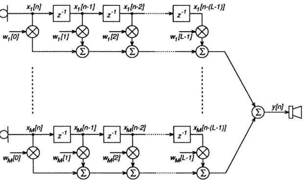
After the received signals have been sampled, they are converted from analog to digital form for subsequent digital processing2_{. The processing schemes under} con-sideration form output samples, y[n], by weighting and combining a finite number of present and past input samples. If the weights are fixed, the processing amounts to LTI FIR (linear-time-invariant finite-impulse-response) filtering. In our case, however, the weights are adaptive and depend on the input and/or output signals. Strictly speaking, then, the processing will be neither linear, time-invariant, nor even finite-impulse-response (when the weights depend on the output samples). If the adaptation is slow enough, however, the system will be almost LTI FIR over short intervals. After the output samples are computed, they are converted from digital to analog form and passed through a low-pass reconstruction filter that produces y(t) for presentation to the listener.

There are at least two ways, shown in Figures 2.4 and 2.5, to view the operation of the digital processing section. Figure 2.4 shows the processing in full detail. Each discrete-time microphone signal passes through a string of L - 1 unit delays, making the L most recent input values available for processing. The complete set of ML values are multiplied by individual weights, w,[l] (where m = 1 ... M and I = 0... L - 1), and added together to form the output y[n]. This processing can be expressed in algebraic terms by the equation

x [n]

y[n] = Tx[n] = [ T[0] wT[] .. WT[L - 11] n , (2.41)

x-[n-L + 1]

where w[l] is the vector of weights at delay 1, and x[n], as defined in the previous section (equation (2.12)), is the vector of sampled microphone signals at time index

2

Although this conversion process introduces quantization errors, we will usually assume that the errors are small enough to ignore and use Equation (2.3) to describe both digital and analog samples.

·IIlllll··-·lll(·C- -I_ -·II I ___C_ ·- I · __ __

w1loJ

xM[n-(L-1)]

WM[Ol

Figure 2.4: Detailed view of signal processing operations.

n. Specifically,

w

[]

xl[n]

[I] = 21 and z[n] [n

WM[] XM [n]

If the weights, w, are adaptive, they will, of course, depend on the time index,

n. We have not expressed this dependence in our notation because changes in

w are normally orders of magnitude slower than changes in x and, therefore, the weights comprise a quasi-LTI system over short intervals. The notation was chosen to emphasize the interpretation of the weighting vector as a filter.

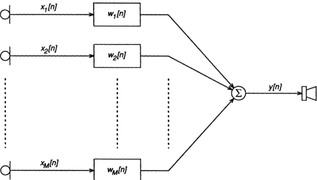
If we consider the weights for each channel as a filter, then we can view the processing more abstractly, as shown in Figure 2.5, where each microphone signal passes through a filter with impulse response w,[n]. In this view, the output is

CHAPTER 2. xl n] BACKGROUND I S ! e ! ! S S * S * S * S S S S S S S * S S S S S e S! I !~~~~~~~~~~~~~ r . ( ! e xM[ln]

Figure 2.5: Filtering view of signal processing operations. simply the sum of M filtered input signals,

y[n] M = E wm[n] * xm[n] m=l M L-1 = Z wm[l] m[n - I] m=l 1=0 L-1 M = E E wm[] m[n - ] 1=0 m=l1 L-1 W= wT [l]x[n-l] 1=0 = wT[n]* [n]

or, in the frequency domain,

M

Y(f)

Z

m=1

If the xm[n] are stationary random processes, we can use (2.43) and, follow-ing (2.22) and (2.23), determine the output autocorrelation and spectral-density 26 (2.42) (2.43) (2.44) 1 1_1_1_ _11__ I_ _I _ · _ 1·11 1 __I_ ___ 1__ I I I I I I I I I

functions:

Ryy[k] = wT[k] * Rz[k] * w[-k] (2.45)

S,,(f) = W T (f(f)S(f) W*(f) . (2.46) We can also use (2.41) and (2.26) to derive the multiplicative form of the output autocorrelation function:

Ryy[k] = E {y[n]y[n n-k]}

= E {wT x[n] xT[n k] w}

- wT Rxx[k ]w, (2.47)

where Rxx[k] is an ML x ML matrix of correlations among all the delayed mi-crophone samples in the array, which can be expressed in terms of the M x M correlation matrix Rz[k].

R

x[nn

[k-

[n-k

RzR[]

R]

R[k

1]

--Rxx[k] = E [n - 1] xtn-k-1] Rzz[k-1] Rx[k] ..

(2.48) Rxx[k] can also be expressed in terms of target and interference statistics. The vector of ML array observations, x, can be modelled by extending (2.12):

x[n] x[n] = [n-1] x[n - L + 1] h[O] h[1] .

0

h[O] ...

CHAPTER 2. BACKGROUND

Using this model,

Rxx[k] = E {x[n]xT[n - k]} = H Rss[k] HT + Rzz[k], (2.50)

where Rss[k] and Rzz[k] are extended versions of Rss, [k] and R, [k].

2.3.3

Response Measures

Once an array processor (a set of microphone locations and weights) has been specified, we can evaluate the response of that processor in at least two ways. The array directional response, or sensitivity to plane-waves as a function of arrival direction, can be determined from the specification of the array processor alone. When we know, in addition, the statistics of a particular signal or noise field, we can determine the overall signal- or noise-field response of the array for that specific field.

Directional Response

An array's directional response can be defined as the ratio of the array processor's output to that of a nearby reference microphone as a function of the direction of a distant test source that generates the equivalent of a plane wave in the vicinity of the array. We will assume that our arrays are mounted in free space with no head present and that the microphones are omnidirectional, and small enough not

to disturb the sound field3. We will also assume that the microphones have poor

enough coupling to the field (due to small size and high acoustic impedance) that inter-microphone loading effects are negligible.

Let the location of microphone m be r, its three-dimensional coordinate vector relative to a common array origin; let a be a unit vector in the direction of signal propagation; let c be the velocity of propagation; and let ST(f) represent the test signal as measured by a reference microphone at the array origin. Then the

3_{The presence of a head or of microphone scattering will introduce direction- and}

frequency-dependent amplitude and phase differences from the simplified plane-wave field that we have as-sumed. The directional response is then harder to calculate and dependent on the specific head and/or microphone configuration.

-tlllll·-C I I--

amplitude and phase of the signal at microphone m will be given by

Xm(f, 5) = ST(f)ej2 fm(a) = ST(f)e-2" , (2.51)

where rm(a) = c'* rfm/c represents the relative delay in signal arrival at microphone m. The array output for the test signal is then

M M

YT(f, 5 ) = W,(f)X(f, 5) = W(f)(f)S~(f)e - j 2 rf Tm( a) (2.52)

m=l m=l

and the array's directional response (sometimes called the array factor) is given by M

g(f, a) Y= )

Z

ST(f) m_

Since a can be expressed in terms of azimuth angle, , and elevation angle, , we can also write the directional response as g(f, 0, /).

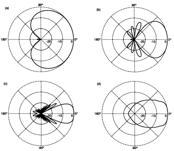
An array's directional response is often described by considering only sources in the horizontal plane of the array and plotting the magnitude of 9(f, 0, 0) at a particular frequency f as a function of arrival angle 9. To illustrate the utility of such beam patterns, Figure 2.6 shows patterns for an endfire array (whose elements are lined up in the target direction, 00) of 21 elements spaced 3 cm apart for a total length of 60 cm, or about 2 feet. The processor that gave rise to these patterns, a delay-and-sum beamformer, delayed the microphone signals to make target waveforms coincident in time and then summed all microphones with identical weights. That is, for a delay-and-sum beamformer,

Wm(f) = ej2fTm(0° ) (2.54) The single-frequency beam patterns of Figure 2.6 (a), (b), and (c) illustrate the fact that delay-and-sum beam patterns become more "directive" (preferentially sensitive to arrivals from 00) at higher frequencies. In quantitative terms, the 3 dB response beamwidth (Elliott, 1981, page 150) varies from about 160° at 250 Hz to 76 at 1 KHz to 38° at 4 KHz. Alternatively, directivity can be characterized by the directivity factor or directivity index, D, defined as the ratio of the response power

BACKGROUND

(d)

1800

-900

Figure 2.6: Beam patterns for a 21-element, 60 cm endfire array of equispaced microphones with delay-and-sum beamforming. Patterns are shown for (a) 250 Hz, (b) 1000 Hz, (c) 4000 Hz, and (d) the "intelligibility-weighted" average of the response at 257 frequencies spaced uniformly from 0 through 5000 Hz. Radial scale is in decibels.

at 0° to the average response power over all spherical angles (Schelkunoff, 1943; Elliott, 1981):

D(f)

(f,

=

1

J

(2.55)

For our 21-element array, we can use an equation for the directivity of a uniformly-weighted, evenly-spaced, endfire array (Schelkunoff, 1943, page 107), to calculate the directivities of patterns (a), (b), and (c) as 3.7, 9.3, and 16 dB, respectively.

The final pattern in Figure 2.6 presents a measure of the array's broadband (c)

180°

-900

I_ I_ _I·_ __ I_ I___ I 1_1 _II_·___ ·_ _ I

directional response, the "intelligibility-average" across frequency of the array's directional response function for sources in the horizontal plane. This average is designed to reflect the net effect of a particular frequency response on speech intelligibility and can be calculated as

()

=

0)l)

(s=

IH(v)1

rmsl/3(H(f)l= (21/6 - 2-1/6)f . (2.57)

This smoothing reflects the fact that, in human hearing, sound seems to be analyzed in one-third-octave-wide frequency bands, within which individual components are averaged together4. The smoothed magnitude response is then converted to decibels to reflect the ear's logarithmic sensitivity to the sound level in a band. Next, the smoothed frequency-response in decibels is multiplied by a weighting function, WAI(f), that reflects the relative importance of different frequencies to speech intelligibility. The weighting function is normalized to have an integral of 1.0 and is based on results from Articulation Theory (French and Steinberg, 1947; Kryter, 1962a; Kryter, 1962b; ANSI, 1969), which was developed to predict the intelligibility of filtered speech by estimating the audibility of speech sounds. Finally, the integral of the weighted, logarithmic, smoothed frequency-response gives the intelligibility-averaged gain, (), of the system. In the special case of frequency-independent directional response, i.e. (f, 0) = K(O), smoothing and weighting will have no effect and ((80)) I = 20 log1 0K(8).

Intelligibility-averaged gain can be described as the relative level required for a signal in the unprocessed condition to be equal in intelligibility to the processed

4

0f course, the presumed smoothing of human audition must operate on the array output signal, and smoothing the magnitude response function (which is only a transfer function), as in (2.56) will be exactly equivalent only when the input spectrum is flat. When the input spectrum is known, we could calculate ()I more precisely by comparing smoothed input and output spectra. However, the simplified formula of (2.56) gives very similar results as long as either the input spectrum or the response magnitude is relatively smooth, and can be used to compare array responses independent of input spectrum.

CHAPTER 2. BACKGROUND

signal. For the broadband beam pattern in Figure 2.6(d), the gain at 0° _{is 0 dB} because signals from 0° are passed without modification and intelligibility is not changed. At 450, the intelligibility-averaged broadband gain of -12 dB implies that processing has reduced the ability of the jammer to affect intelligibility to that of an unprocessed jammer of 12 dB less power.

The absolute effect of a given jammer on intelligibility will depend on the characteristics of the target. As an example, consider first a "reference" condition with target and jammer coincident at 00, equal in level, and with identical spectra. In this situation, Articulation Theory would predict an Articulation Index (the fraction of target speech elements that are audible) of 0.4, which is sufficient for 50% to 95% correct on speech intelligibility tests of varying difficulty. Now, if

that same jammer moves to 450, its level would have to be increased by 12 dB

to produce the same Articulation Index and target intelligibility as the reference condition5. Alternatively, the target could be reduced in power by 12 dB and still be as intelligible as it was in the reference condition. This implies one last interpretation of ({)I as that target-to-jammer ratio necessary to maintain constant target intelligibility (similar to the predictions of Zurek's binaural intelligibility model in section 2.1).

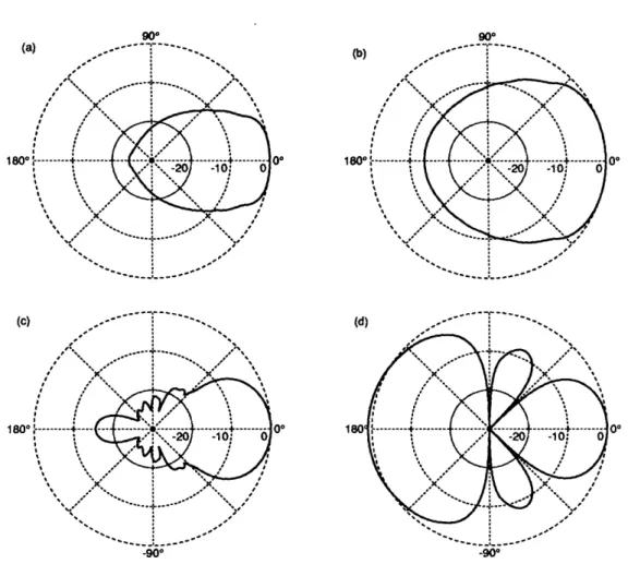
Based on intelligibility-averaged broadband gain, the four broadband beam patterns in Figure 2.7 can then be used to illustrate the rationale for adaptive beamforming. Pattern (a) is; once again, the average directional response of a 21-element 60-cm (2-foot) delay-and-sum endfire array. Although its directivity might be satisfactory for a hearing aid, its size is excessive. Pattern (b) is the result of reducing the delay-and-sum beamformer array to six elements over 15-cm (0.5 foot). Now the size is acceptable but directivity has decreased substantially. Patterns (c)

and (d) show the results of applying "optimum" beamforming (to be discussed in

5

Strictly speaking, (), only approximates the result of a search for the input Target-to-Jammer-Ratio that would give an A.I. of 0.4 if the A.I. calculation were performed in full (non-linear) detail. However, for a number of cases in which full calculations were made, the approximation error was less than 0.5 dB if the range of the frequency response was less than 40 dB. For frequency responses with ranges greater than 40 dB, the approximation was always conservative, underestimating the effective jammer reduction.

_____il__l __ __

_I 1______·1

(a 1800 (b) II \ 180- i.--· I II II (c) 180° 00 .900 -90

Figure 2.7: Broadband beam patterns for four equispaced, endfire arrays: (a) 21 elements, 60 cm, delay-and-sum beamforming; (b) 6 elements, 15 cm, delay-and-sum beamforming; (c) 6 elements, 15 cm, weights chosen to maximize directivity; (d) 6 elements, 15 cm, weights chosen to minimize jammers at 45° and -90° .

the next chapter) to the same 6-element, half-foot endfire array. In pattern (c), the processing weights have been optimized to maintain the target signal but minimize the response to isotropic noise or, equivalently, to maximize the directivity index (Duhamel, 1953; Bloch, Medhurst and Pool, 1953; Weston, 1986). This processing scheme provides directivity similar to that in pattern (a) with an array four times smaller. It should be noted, however, that endfire arrays designed to maximize directivity (so called "superdirective" arrays) are often quite sensitive to sensor noise and processing inaccuracies (Chu, 1948; Taylor, 1948; Cox, 1973a; Hansen, 1981). For hearing aid applications, this sensitivity may be reduced while significant

CHAPTER 2. BACKGROUND

directivity is retained by using "suboptimum" design methods (Cox, Zeskind and Kooij, 1985; Rabinowitz, Frost and Peterson, 1985; Cox, Zeskind and Kooij, 1986). In pattern (d), the processing weights have been optimized to minimize the array output power for the case of jammers at 450 and -90 ° _{in an anechoic environment} with a small amount of sensor noise. Although the beam pattern hardly seems directional and even shows excess response for angles around 180°_{, only the} re-sponses at angles of 0°_{, 45}°_{, and -90} ° _{are relevant because there are no signals} present at any other angles. Pattern (d) is functionally the most directive of all for this particular interference configuration because it has the smallest response in the jammer directions. If the interference environment changes, however, the processor that produced pattern (d) must adapt its weights to maintain minimum interference response. This is precisely the goal of adaptive beamformers.

Signal- and Noise-Field Response

When we know the characteristics of a specific sound field, such as the field generated by the two directional sources in the last example, we can define the array response to that particular field as the ratio of array output power to the average power received by the individual microphones. This response measure takes into account all the complexities of the sound field, such as the presence of multiple sources or correlated reverberant echoes from multiple directions.

We will use K,(f) to denote an array's noise-field response at frequency f to noise with an inter-microphone cross-spectral-density matrix of Snn(f). The noise-field response will depend on Snn(f) and on the processor weights, W(f), as follows. The average microphone power is the average of the diagonal elements of Snn(f) or trace(Snn(f))/M. The array output power, given by equation (2.46), is simply WT(f) Snn(f) W*(f). The array's noise-field response is then

K(f) = () trace(S) (f)) (2.58)

A similar array response can be defined for any signal or noise field. In particular,

-s-L--·lll·--- _-·1_11--_1_--- --11111 -·^I1 __ _ _

we will be most interested in the response to the total noise signal, z:

W T(f) Sz(f)

w*(f)

K(f)= !trace(Sz(f)) ; (2.59)

the response to sensor noise, u, whose cross-correlation matrix is o2 IM:

WT(f)a 2

=

(2.60)

Ku(f) _{9 trace(a} l t =

e(

)

w(f)

and the response to the received target signal, r[n] = h[n] * s[n], from (2.32): K( WT(f) r(f) W*(f) WT(f)

t(f)

(f)

t(f)

t

trace(Srr(f)) trace((f)S,,(f) (f))

wT(f) t(f)

Xt(f)

1 trace(2it(f) H(f)) 1 l(f)I2 (2.61)

where we have factored out the scalar signal power, S,,(f) and used the identity trace(AB) = trace(BA).

A measure of array performance that often appears in the literature, array gain GA, is the ratio of output to input signal-to-noise ratios (Bryn, 1962; Owsley, 1985; Cox, Zeskind and Kooij, 1986) and is easily shown to be

GA(f) = Kr(f) (2.62)

Note that array gain could be described as the gain against the total noise field and is opposite in sense to the total-noise response, K(f), but has the intuitive appeal that higher gains are better. We will extend the array gain notion by defining similar gains for particular noise-fields of interest. Specifically, if we use G,(f) to denote the ratio of output to input signal-to-noise ratios for noise n, then we can define a total-noise gain,

GK(f) = GA(f) (2.63)

K,(f)

which is identical to array gain; an isotropic-noise gain, or array gain against isotropic noise,

Gi(f) = K(f) = D(f) (2.64)

Ki(f)

CHAPTER 2. BACKGROUND 36

which is identical to the array directivity defined in (2.55); and a jammer-noise gain, or gain against received directional-jammer signals,

Gj(f) = K(f)I

Kj(f) '

where Ki(f) and Kj(f) are the array responses, defined as above, to isotropic and directional-jammer noise fields, respectively6.

6

This family of gain measures is missing one member that we will not use. A commonly-used measure of array insensitivity to errors, white noise gain, or gain against spatially- and temporally-uncorrelated noise is defined as

K. (f)

Gw(f) = G,(f) = Ku(f) (2.66) This measures the degree to which the signal is amplified preferentially to white noise and random errors (Cox, Zeskind and Kooij, 1986). Thus, larger values of Gw are better, although the signifi-cance of a small Gw will depend on the amount of white noise or the magnitude of error actually present. In fact, Gw predicts the ratio by which white noise would have to exceed the signal to produce equal power in the output. Note that white noise gain, Gw, is inversely proportional to the sensor-noise response, Ku. In the common special case where the signal gain, Kr, is unity,

1uIf

Gw(f) = K - W(f)1 _{(Kr = 1) .} (2.67)

We prefer to use Ku(f) directly as a measure of the sensitivity of a processor to sensor-noise.

I-Y--Optimum Array Processing

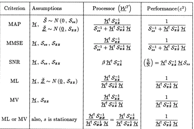
In the last chapter we described the signal-processing structure of our proposed multi-microphone monaural hearing aid and used response patterns to illustrate the potential benefit of processing that is matched to the received interference. In this chapter we derive specific processing methods that are, in various senses, "optimum" for removing stationary interference. In subsequent chapters we will analyze the performance of these optimum processors and describe adaptive process-ing methods that can approach optimum performance in non-stationary hearprocess-ing-aid environments.

Our investigation of optimum processing will proceed in three steps. First, we will consider various optimization criteria for processing based on unlimited observations (i.e., processing that uses data from all time) and show that the various criteria lead to similar frequency-domain processors. Second, we will consider a few of the same criteria for processing based on limited observations, which will lead to optimum time-domain processors. Third, we will try to relate the frequency- and time-domain results and discuss ways in which the different methods can be used.

3.1

Frequency-Domain Optimum Processors

Although our ultimate goal is an AMMA based on a limited number of micro-phone signal samples, as shown in Figure 2.4, we can gain considerable insight with relatively simple calculations by first considering the case in which samples from all time are available. If the sampled signal is stationary, it will have a spectral representation, similar to the Fourier transform of a deterministic signal, that depends on the signal samples over all time. Because the components of the signal's spectral representation at different frequencies will be uncorrelated, the

CHAPTER 3. OPTIMUM ARRAY PROCESSING

derivation and application of optimum processors in the frequency domain will be greatly simplified. The results of frequency-domain processing can then be used to bound the performance of realizable processors based on a limited number of samples.

Spectral Representation of a Random Process. To present a rigorously correct definition of the spectral representation of a stationary random process would involve mathematical issues beyond the scope of this thesis (Wiener, 1930; Doob, 1953; Van Trees, 1968; Gardner, 1986). We will use an approximation that is essentially correct but requires a bit of justification.

Over a finite interval, a function x[n] can be represented as a sum of orthonormal basis functions;

N-i

x[n] = Xk q lk[n] (-N/2 < n < N/2) (3.1)

k=O

where the basis functions, k[n], satisfy

N/2-1

ZE

n=-N/2

and the Xks can be determined by

N/2-1

Xk= E x[n]4[n] . (3.3)

n=-N/2

If the basis functions are known, then the set of XkS, {Xk I 0 < k < N}, and the values of x[n], {x[n] I - N/2 < n < N/2}, are equivalent representations of the same function.

When x[n] is a random process, its values will be random variables and the Xks will be linearly related random variables. Karhunen and Loive have shown that it is possible to choose a set of basis functions such that the Xks are uncorrelated (Van Trees, 1968), i.e.

E {Xj Xk} = Aj 6[j- k]

_II _·_II _I_ _I_ __I··__ I^·__·_^I __ ___ _ ___

38

Assuming that x[n] is stationary, this special set of basis functions will satisfy

N/2-1

E7

R[n

m=-N/2

in which

qk

oo,

this equation approaches the form of a convolution of Ok with R, which can be viewed as the impulse response of an LTI system, whose eigenfunctions must be complex exponentials.

In fact, it can be shown (Davenport and Root, 1958; Van Trees, 1968; Gray, 1972) that for large N,

Ok[n] N ej 2 k n / N -r 1 ej 2rfknT (3.6)

) \ = Sc(fk), (3.7)

where fk = k . (The previously mentioned mathematical issues arise in rigorously taking the limit of these expressions as N -- oo.) This leads to our approximate (for large N) spectral representation,

1 N/2-1

XN(f)

for which

E {XN(fj) (fk)} _ SZ(f/) 6[j - k] (3.9) The validity of this approximation will depend on N being much greater than the non-zero extent of Rx,[n] or, equivalently, greater than some function of the "sharpness" of features in Sx,(f).

We can now proceed to consider various optimizing criteria in the derivation of frequency-domain optimum processors.1 These derivations will all be based on a model of the received signal, generalized from Section 2.3.1, as

XN(f) = 21(f) SN(f) + gN(f) (3.10) 1The basic concept and many of the results of this section were originally presented by Cox in an excellent paper (Cox, 1968) and later expanded slightly by Monzingo and Miller (Monzingo and Miller, 1980).