Aeroelastic analysis and sensitivity calculations using the Newton method

Aeroelastic Analysis and Sensitivity

Calculations Using the Newton Method

by

Thomas Mead Sorensen

SUBMITTED TO THE DEPARTMENT OF AERONAUTICS AND ASTRONAUTICS

IN PARTIAL FULFILLMENT OF THE REQUIREMENTS FOR THE DEGREE OF

Doctor of Philosophy at the

Massachusetts Institute of Technology September, 1995

@1995, Massachusetts Institute of Technology

Signature of Author F - - ,FP

-Dep ent Aerona tic lAstronautics

, ' ' Of) June 8, 1995 Certified by Certified by Certified by Certified by Thesis Supervisor,

\IProf.

Mark Drela

\ - --- " f. Jaime Peraire

Associate Professor of Aeronautics and Astronautics

r-Prof. Hugh L.N. McManus Assistant Professor of A onajintn4.trautics

I rof. Anthony T. Patera

B. ofessor ofMeaanical Engineering Accepted by

Prof. Harold Y. Wachman

OF;A CHNL " , Depit'meit Giaiiate' Committee

OF TECHNOL

SEP

2 5

1995

.

Aerr

Aeroelastic Analysis and Sensitivity

Calculations Using the Newton Method

by

Thomas Mead Sorensen

Submitted to the Department of Aeronautics and Astronautics on June 22, 1995

in partial fulfillment of the requirements for the degree of Doctor of Philosophy in Aeronautics and Astronautics

A method is developed for calculating design sensitivities of an aeroelastic system using a Newton-based code. The Newton method provides a single framework: 1.) to solve the nonlinear steady aerodynamic problem, 2.) to solve the harmonic-unsteady aeroelastic eigenvalue problem, and 3.) to compute the solution sensitivities. The aerodynamic behavior is modeled using a Galerkin Finite Element discretization of the Full Potential equation. The Newton method is used to restrict the Unsteady Full Potential equation to small amplitude harmonic response. A modified wall transpiration boundary condition is derived which is not restricted to normal displacements, but still retains the ease of implementation of the traditional wall transpiration boundary condition. A two degree of freedom undamped typical section is used to model the structural response. Sensitivities are calculated with respect to steady and unsteady general shape design variables, nondimensional structural parameters, and aerodynamic design variables. The solutions from the steady and unsteady codes are compared with existing experimental and computational data. A comparative example between the eigenproblem sensitivities calculated by the Newton-base code and by finite differencing is presented.

Thesis Supervisor: Mark Drela,

Acknowledgments

With the completion of this thesis I have earned a Ph.D., but to my wife Dorene goes the much more difficult degree of Ph.T. (Pushing Hubby Through). I couldn't have made it this far without her constant love and support. I look forward to a lifetime of

trying to repay her for her six years of sacrifice.

I also owe a tremendous amount of thanks to my advisor and friend Mark Drela. I am especially grateful for the leeway he granted me to work on MIT's human powered hydrofoil, Decavitator. Building the hydrofoil was certainly the highlight of my time spent at MIT and I am proud to have worked with such a fine group of people.

Lastly, my sincere appreciation to all of the inmates of the CASL and its predecessor, the CFDL. Good luck to all of you in your future endeavors.

This research was supported by the Raytheon Company, with Dr. Peter Digiovanni as Technical Monitor and the Boeing Company, with Dr. Wen-Huei Jou as Technical Monitor.

Contents

ions of Present Work . . . .

f Thesis . . . .

2 The Newton Method

2.1 Introduction ...

2.2

2.3

Steady Analysis Newton System ...

2.4 Design Newton System . . . .

2.4.1 Special Case: Parameters Dependent on

2.4.2 Special Case: Linear Residuals . . . . .

2.5 Eigenproblem Newton System . . . .

2.6

2.7

2.8

the Design Variables

Jacobian Assembly Procedure . . . .

Matrix Equation Solver . . . .

Aeroelastic Analysis/Design Newton System

3 Governing Equations

3.1 Aerodynamic Equations ...

3.1.1 Unsteady Full Potential Equation . . .

3.1.2 Boundary Conditions (BC) ...

3.1.3 Linearized Steady and Unsteady Forms

3.1.4 Finite Element Method Discretization

3.2 Structural Equations ... 3.3 Validity ... 3.3.1 Aerodynamic Equations ... 3.3.2 Structural Equations ... 4 Design 4.1 Introduction ... ... .. .. ... .... 40 . . . . 40 S . . . . . 41 . . . . 43 S . . . . . 48 S . . . . . 49 . . . . 49 . . . . 51 . . . . 51 . . . . 52

. . . . 54

4.2.1 Linear Design Perturbations ... . 54

4.2.2 Nonlinear Design Perturbations . ... 55

4.2.3 Linear and Nonlinear Inverse-Design . ... 57

4.3 Shape Design Variables ... 60

4.3.1 Derivation ... .. 61

4.3.2 Use of Mode Shapes ... 65

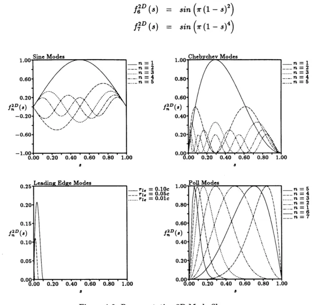
4.3.3 Creating 3D Mode Shapes ... ... 66

4.3.4 Examples of 2D Mode Shapes ... 67

4.4 Structural Design Variables ... 69

4.5 Aerodynamic Design Variables ... 69

4.6 Steady versus Unsteady Design Variables . ... 69

5 Results 71 5.1 Steady Examples ... ... 71

5.1.1 Steady Analysis ... 71

5.1.2 Steady Design Perturbations ... . 75

5.1.3 Steady Inverse-design ... 85

5.2 Unsteady Examples ... ... 87

5.2.1 Unsteady Analysis ... 87 4.2 Utilizing the Sensitivities

5.2.2 Unsteady Design Perturbations . . . .

5.3 Aeroelastic Examples ... ...

5.3.1 Aeroelastic Design Perturbation - Sensitivity Comparisons . . .

6 Conclusions

6.1 Newton System Benefits ...

6.2 Sensitivity Calculations ...

6.3 General Wall Motions ...

6.4 Code Development ...

6.5 Aeroelastic Calculations ...

6.6 Linearization ... ...

6.7 Uses for the Code ... ... . .. ...

7 Recommendations for Future Work

7.1 Boundary Layer Effects ...

7.2 Faster Sensitivity Calculations . . . .

7.3 Three-Dimensional Structural Model . . . . .

7.4 Adding Flutter Speed to the List of Unknowns

7.5 Complex Grids ...

7.6 Supersonic Freestreams . . . .

7.7 Full Aeroelastic Problem . . . .

93 96 96 99 99 100 100 101 101 102 102 105 105 106 107 108 109 109 109

7.7.1 Static Aeroelastic Response ...

7.7.2 Gust Response ...

Bibliography

A Model Problem Examples

A.1 Example 1: Harmonic-Unsteady Analysis ...

A.1.1 Small Amplitude Harmonic Response Derivation ...

A.1.2 Newton Method Derivation ...

A.2 Example 2: Design Sensitivity Calculation ...

A.2.1 Analytic Sensitivity Calculations ...

A.2.2 Newton Sensitivity Calculations . . . .

B Linearization of the Aerodynamic Equations

B.1 Linearization ...

B.1.1 Gust Response ...

C FEM Discretization of the Aerodynamic Equations

C.1 Hexahedral Mesh Element . . . .

C.2 FEM ...

C.3 Shape Function Gradients ...

* 110 . 110 111 116 116 116 . 117 118 119 119 121 121 . 126 127 . 127 128 . . .. ... ... . 129 C. ... . 130 C.4 Integration ...

D Harmonic-Unsteady Jacobian Matrix 131

D.1 Assembled Form ... 131

D.2 Quasi-steady Flow ... ... 132

E Design Variable Derivatives 133

E.1 Normal Vector Derivatives ... 133

E.2 Derivatives of Aerodynamic Equations ... ... 135

List of Figures

2.1 Three Uses for the Newton Method ... .. 26

3.1 Boundary Conditions ... 44

3.2 Wall Boundary Condition Parameters ... 47

3.3 Change in T and n Due to Wall Motion ... 48

3.4 Typical Section Model: Airfoil Constrained by Bending and Torsion Springs 50 4.1 Schematic Comparison of the Linear and Nonlinear Approximation Meth-ods versus the Exact Solution ... 56

4.2 Sensitivities Calculated After Each Newton Step . ... 59

4.3 Geometry Perturbations and Wing Surface Parameterization ... 62

4.4 Mode Shapes: a.) Normal Mode; b.) Breakdown of Normal Mode for Finite Displacement; c.) General Mode . ... 63

4.5 Wall Rotation ... 66

4.6 Representative 2D Mode Shapes ... 68

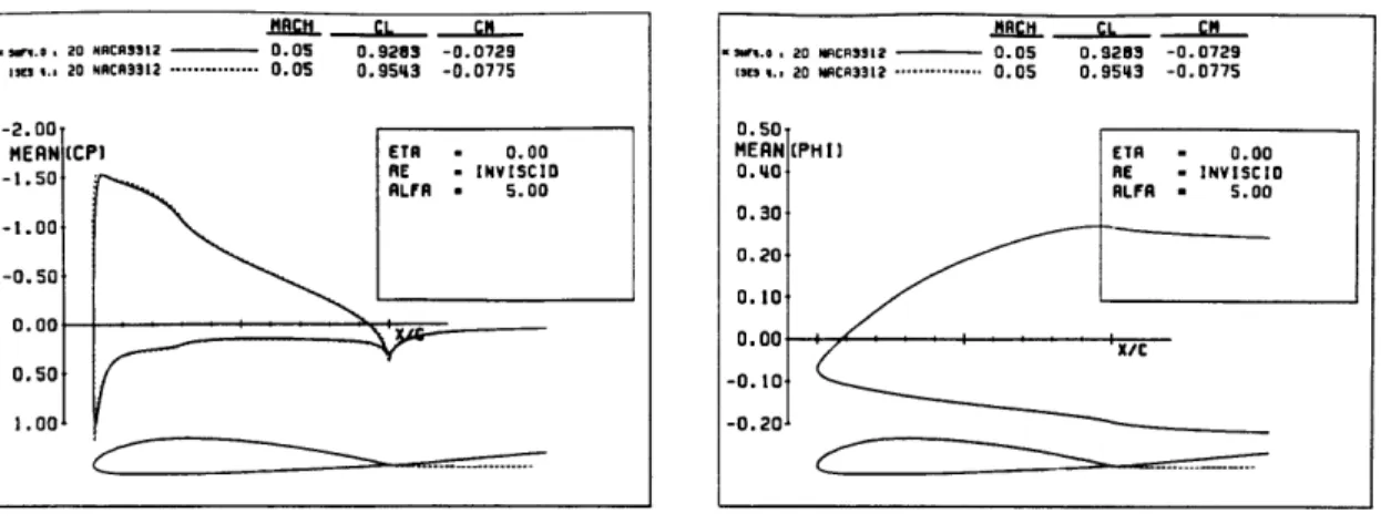
5.1 2D Steady Analysis - Incompressible: Comparison with ISES ... 72

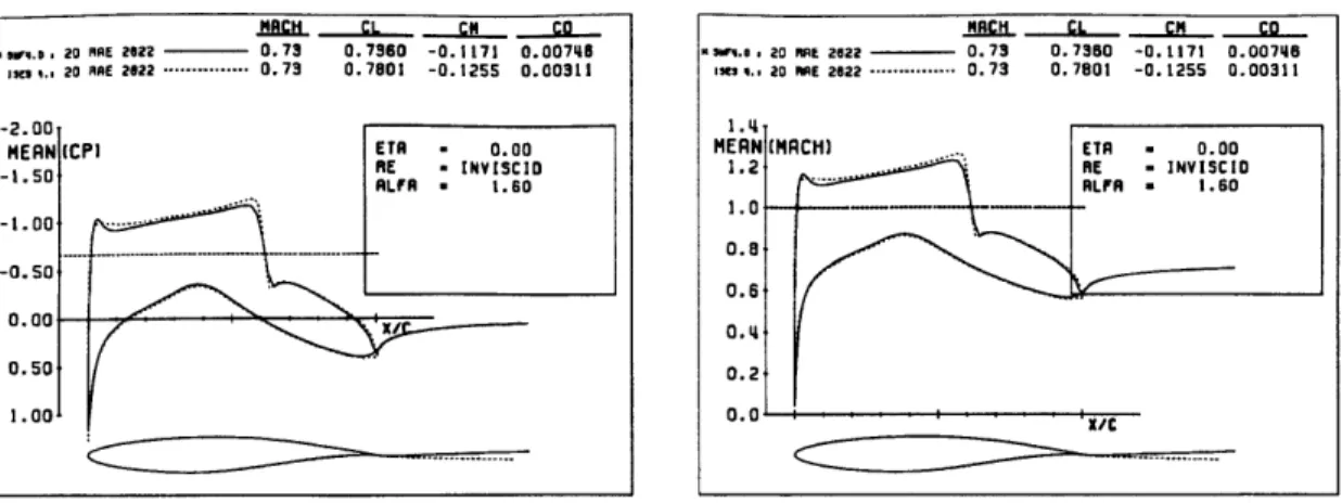
5.2 2D Steady Analysis - Supercritical : Comparison with ISES ... . 73

5.4 2D Steady Design Perturbations - Sensitivities: Calculated versus Finite Difference (camber design variables) .... . ... 76

5.5 2D Steady Design Perturbations - Sensitivities: Calculated versus Finite Difference (thickness design variables) . ... 77

5.6 2D Steady Design Perturbations - Subcritical Design: Pitch Mode . . . 79

5.7 2D Steady Perturbation - Subcritical/Supercritical Design: NACA 3312 M ode . . . 80

5.8 2D Steady Perturbation - Supercritical Design: NACA 0013 Mode . . . 81

5.9 2D Steady Perturbation - Aerodynamic Design Variable: M, ... 82

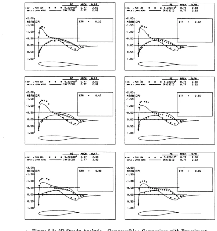
5.10 3D Steady Perturbation - Comparison of C, Distributions ... 83

5.11 3D Steady Perturbation - Comparison of Cp Contours . ... 84

5.12 2D Steady Inverse-design - Two Design Variables: a.) Comparison of the Seed, Approximate, and Target Solutions; b.) Comparison of Exact and Approximate Solutions ... ... . 85

5.13 2D Unsteady Analysis - Comparison with BVI : Mean Solution .... . 88

5.14 2D Unsteady Analysis - Comparison with BVI: a.) Pitch Solution, k -=

0.005; b.) Pitch Solution, k = 0.05; c.) Plunge Solution, k = 0.5 . . . . 89

5.15 2D Unsteady Analysis - Comparison with BVI : Forces Versus Reduced Frequency for Pitch Case ... 90

5.16 2D Unsteady Analysis - Comparison with BVI : Forces Versus Reduced Frequency for Plunge Case ... 91

5.17 2D Unsteady Analysis - Comparison with Experiment : Subcritical. . . 92

5.19 3D Unsteady Analysis - Comparison with Experiment : Supercritical 94

5.20 2D Unsteady Perturbation - STEADY Design Variable: a ... . 95

5.21 2D Unsteady Perturbation - UNSTEADY Design Variable: 9 ... 95

5.22 2D Unsteady Perturbation - UNSTEADY Design Variable: k ... 96

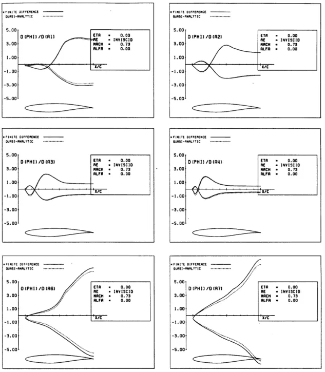
5.23 Representative Examples of Calculated Sensitivities Compared to Finite

Difference Calculations ... 97

6.1 Typical Design Cycle ... 104

7.1 Steady Flap Perturbation [51] ... 106

7.2 2D Steady Supersonic Examples - a.) Analysis, and b.) Design Perturbationll0

C.1 Hexahedral Mesh Element in Physical Space and Natural Coordinates . 128

List of Symbols

k

p, /3

C

h,

0

N

residual, unknown, design variable time dependent parameter

design variable dependent parameter generic variable

dimensional frequency

- f = a + i w, nondimensional complex frequency

- 2 2V reduced frequency

density, upwinded density

pressure, temperature, velocity vector, specific heat ratio vorticity vector

perturbation velocity potential Mach number, angle of attack position vector, unit normal vector upwinding switch and control parame.ers mean aerodynamic chord

lift, moment coefficients at c

moment coefficient calculated at elastic axis pressure coefficient

harmonic plunge and pitch amplitudes wing span, nondimensional span location

FEM Shape Function

body surface geometry, velocity, and position vector structural parameters

natural frequency of torsional oscillation of airfoil inverse-design variables

general mode shape

jth _{normal mode shape, total normal wall perturbation}

wall transpiration velocity

Superscripts and Subscripts

quantity for seed geometry

approximate quantity for new geometry quantity for new geometry

quantity for target geometry

rth cycle of Newton procedure

freestream quantity upwind variable upper and lower wake

aerodynamic variable, structural variable, eigenvalue

Miscellaneous Symbols

gradient with respect to space variables perturbation quantity

vector

mean and harmonic quantities real and imaginary parts of ( )

ri k CP M ( )/0,ma,

f

)UP

)U, ()

6( )

( )

(), (()

Symbols Used in Plots

ETA R. FREQ.

CP

( )/A

D(PHI)/D(A1)

MEAN() ()

HARM() ₍₎

REAL( ) or RE() W()

IMAG() or IM() (*))

Chapter 1

Introduction

This chapter will discuss the motivation and goals of this research and its relation to previous work. A discussion of the contributions of this work follows. A brief outline of the topics to be covered in the remaining chapters will be presented at the end of the chapter.

1.1

Motivation

The goal of numerical fluid simulation codes is to improve the performance of some given aerodynamic system. Great strides have been made in analysis codes over the years due to aggressive development of new solution algorithms and the tremendous advances in computer technology. Today the Steady Full Potential equation is regularly solved around realistic three dimensional geometries, while in two dimensions it is now possible to solve the Navier-Stokes equations in a reasonable amount of time.

Steady analysis codes have had an enormous impact on how aircraft are designed by allowing many more candidate configurations to be considered before settling on the final design. Contrary to the initial expectation of some, computational methods did not replace wind tunnels but instead complemented them. The computational methods are used to rapidly compare competing design concepts to find the two or three most promising configurations which are then tested in a wind tunnel. This arrangement frees the wind tunnels to do what they do best - obtaining vast amounts of data [36]. A limitation common to both wind tunnels and numerical analysis codes is that they only provide the user with the flow solution for the given geometry and flow con-ditions, the so-called "zero order information." No information is provided about how

the solution responds to changes in either the flow conditions or the geometry (the first order information or solution sensitivities). First order information can be computed from zero order information using finite differencing techniques. This is done with wind tunnel experiments to calculate, for example, lift curve slopes and stability derivatives. However, first order information with respect to geometry changes is extremely expen-sive to calculate using wind tunnels due to the high cost of building wind tunnel models. Calculating sensitivities using finite differencing is relatively easy to do with numeri-cal analysis codes, but the computer resources required to numeri-calculate sensitivities in this manner are quite large.

Lagging several years behind the maturity of analysis codes are design codes. These come in two basic forms, inverse-design codes and optimization codes. Many techniques are available for each but the best of these codes generally rely on the flow sensitivities to speed the convergence process. In order for this speed to be realized the sensitivities must be calculated as cheaply as possible. Previous work has shown that calculating sensitivities with Newton-based analysis codes is systematic and much more efficient than resorting to finite differencing [13, 42]. The resulting sensitivity information is not limited to optimizers or inverse-design, but can be used for a multitude of design related problems.

Steady analysis and design codes have transformed the manner in.which aircraft are designed. Unsteady and aeroelastic codes are just beginning to make an impact [16]. The methods and equations currently used for unsteady analysis are roughly ten years behind the state of the art for steady codes. Sensitivity information is just as important in the unsteady realm as it is in steady flow, however, unsteady design codes which can calculate sensitivities are only just starting to make an appearance. The development of aeroelastic design codes which calculate sensitivities for combined unsteady aerodynamic and structural dynamic systems is even further behind.

As will be shown in this thesis, the Newton-based quasi-analytic sensitivity calcu-lation procedure is a general technique that can be applied to any system of equations solved using the Newton method. By assuming harmonic response it is possible to solve unsteady aeroelastic problems using Newton's method. It therefore becomes feasible to

produce an aeroelastic analysis code that also calculates sensitivities.

1.2

Goals

The research documented in this thesis had several goals, each concerned with obtaining sensitivity information from aeroelastic systems. A primary goal was the development of a method to calculate frequency and eigenvector sensitivities, along with aerodynamic sensitivities, for a coupled aerodynamic/structural system. A secondary goal was to perform this task completely within the confines of a single Newton-based code structure to allow savings in code development time and a reduction in the number of specialized routines required. Another major goal was to develop a method to simulate geometry perturbations that are not limited to normal displacements but did not require moving the computation grid. To enhance its effectiveness for a designer, this code was also developed to have three levels of accuracy with a proportional cost for each.

1.3

Background

Structural elasticity plays an important role in designing aerodynamic systems, and the purpose of most unsteady aerodynamic codes is to predict aeroelastic behavior [50]. Reflecting this importance, the NATO Advisory Group for Aerospace Research and Development (AGARD) has had several conferences devoted to unsteady aerodynamics and aeroelasticity. Survey papers from two of these conferences provide an excellent background to the issues involved in dealing with aeroelasticity, and some of the com-putational methods used to date [16, 30].

Aeroelastic calculations have traditionally relied on linear subsonic and supersonic computational methods to aid in the design of aircraft. The troublesome transonic region, with its associated "dip" in the flutter stability boundaries, was left to wind tunnel experiments. However, the introduction of LTRAN2, a 2D, time-accurate, Tran-sonic Small Disturbance (TSD) code made it possible to efficiently simulate unsteady

transonic flows [15].

The TSD equations are the simplest equations able to predict the major nonlinear effects associated with flight near Moo = 1. Therefore, most of the unsteady transonic codes to date have used the TSD equation. A further advantage of TSD methods is that, due to the small-amplitude form of the wall surface boundary condition, they work with simple Cartesian meshes [19].

More accurate than the TSD equation is the Full Potential (FP) equation. Unlike TSD the FP equation does not limit the solution to small deviations from freestream flow. One consequence of stepping up to the FP equations is that the simple imple-mentation of the wall boundary condition used by TSD methods must be replaced with equations applied on the actual surface of the body. This usually requires that compli-cated, non-Cartesian meshes be generated around the body (an exception is provided by TRANAIR [23]).

A large number of codes exist for analyzing unsteady aerodynamic and aeroelastic systems, and no attempt will be made to describe them all here. Most rely on TSD or FP, although a few codes use the Euler equations [21, 29, 47]. In addition to the different governing equations used by the various codes, they also vary in the methods used to discretize the equations and the techniques used to solve the discretized equations.

Substantial time savings can be realized for the TSD, FP, or Euler equations by restricting them to harmonic-unsteady response. This assumes that the unsteady flow can be decomposed as an harmonic oscillation about a steady flow solution. The benefit of the harmonic assumption is that time derivatives are replaced by terms involving a frequency. This allows the problem to be solved without time-marching. This method has been applied to 2D cascades using both the FP equation and the Euler equations [21,

44, 45] and to 3D wings using the FP equation [40].

Unsteady analysis codes are useful for predicting the occurrence of unwanted aeroe-lastic phenomena. Although it is possible to avoid the unwanted phenomena by the

addition of mass, stiffness, or damping [17], analysis codes provide little information that can be used to systematically modify the system to obtain the optimal result. A

code which includes sensitivity information, in addition to a pure analysis solution, is more useful in this situation since it provides a first-order answer to the "What if?" questions. For instance, sensitivity information can show how the mass may be redis-tributed, rather than increased, to alleviate undesired aeroelastic phenomena.

A variety of sensitivity analysis codes are currently available for steady aerodynamic problems, but few exist for unsteady aerodynamic or aeroelastic systems [41]. An exam-ple of a sensitivity code for unsteady aerodynamic loads in cascades was presented by Lorence and Hall [28]. The aeroelastic realm includes codes by Barthelemy and Bergen, [2] and Karpel [24].

This thesis presents a method for efficiently calculating aeroelastic sensitivities with respect to structural properties and aerodynamic shape. The method is similar to that of Lorence and Hall [28] but does not require a moving grid. The boundary condition used to approximate the moving body is also used by the sensitivity calculations to overcome the drawback found in many shape sensitivity methods: restriction to normal wall motions [2]. An added benefit is that the present method uses a single Newton method framework to solve the steady and unsteady analysis problems, as well as calculating the sensitivities and solving eigenvalue problems.

1.4

Contributions of Present Work

This thesis describes a method for finding sensitivities for not only unsteady aero-dynamic problems but also aeroelastic problems. The aeroelastic sensitivities include sensitivities for both the frequency and structural eigenvector, in addition to the aero-dynamic variables.

This thesis shows that by fully exploiting the characteristics of the Newton method a unified program structure can be used to solve the seemingly disparate problems of steady and unsteady aerodynamic analysis, aeroelastic response, and sensitivity calcu-lations. The only major difference between all these tasks is that unsteady routines require frequency terms and sensitivity calculations require additional right hand sides.

By fully coupling the aerodynamic and structural equations it is possible to obtain aeroelastic response without resorting to the use of fixed in-vacuo structural solutions. This allows the natural mode shapes and the eigenvalues to change during the solution process.

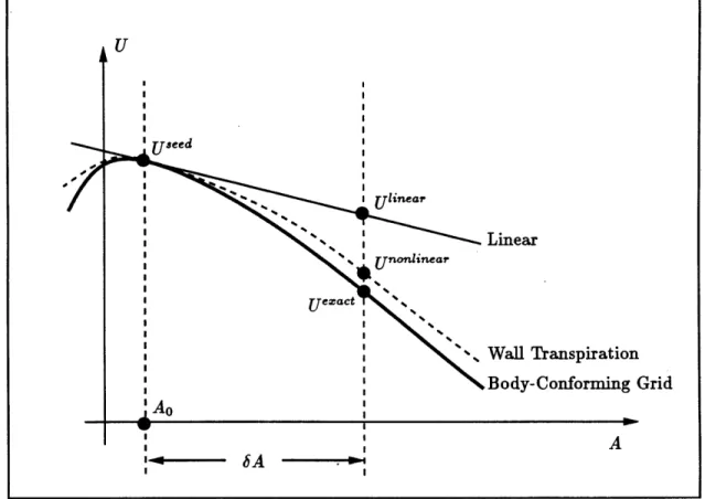
Another benefit of the current method is that it provides three levels of accuracy within one code. The most accurate level is full analysis in which the wing being investi-gated is gridded and solved. The next level allows geometry changes to be implemented and analyzed without changing the underlying grid, which for complicated geometries can be difficult and costly to compute. The lowest level of accuracy allows changes in the solution to be linearly approximated using the sensitivity information. Naturally the cost of each method reflects its level of accuracy.

The linearized wall boundary condition used in this thesis provides a single general method for implementing steady and unsteady wing motions, along with providing con-venient design variables for the sensitivity routines. The same computational routines are used for both purposes, and in common with wall transpiration models, it is easily implemented. However, unlike wall transpiration the present method is not restricted to normal geometry perturbations.

1.5

Outline of Thesis

Chapter 2 describes the similarities between linearized steady, harmonic-unsteady, de-sign, and eigenvalue problems. This is followed by the governing equations and bound-ary conditions in Chapter 3. The derivation of the design variables and examples of their uses are given in Chapter 4. The results are included in Chapter 5. Conclusions are given in Chapter 6 with recommendations for further work in Chapter 7. Several appendices are included which contain detailed derivations.

Chapter 2

The Newton Method

This chapter is devoted to the Newton method and the various ways in which it is used throughout this thesis.

2.1

Introduction

The Newton method is well known as a powerful iterative technique for solving steady nonlinear equations. In this work, the Newton method will be used to perform: 1.) steady analysis, and will be modified to solve three additional problems: 2.) harmonic-unsteady analysis, 3.) sensitivity calculations, and 4.) eigenvalue problems.

The versatility of the Newton method is due to the manner in which a solution is resolved into a summation of a known component, U', and an unknown perturbation, 6U'. The first three uses of the Newton method listed above are shown schematically in Fig. 2.1, where the known and unknown components are identified. These uses are also discussed below:

1. Steady Analysis: The known component, U', is an initial guess for the actual

solution. The unknown perturbation, 60', is the error between the initial guess and the linearized solution which is determined by solving the linearized problem, and then used to update the known component. This procedure is iteratively

continued until convergence.

2. Harmonic- Unsteady Analysis: The mean solution is used as the known component, while the unknown component is the harmonic perturbation. In this case, since the mean solution is assumed to be independent of the unsteady solution no iteration

U- -_

R(U;A)

I

I*U

Figure 2.1: Three Uses for the Newton Method is necessary.

3. Sensitivity Analysis: The change in the solution, bU', due to a change in a given set of design variables, 6A, is desired. Once again, this can be thought of as a known component (the solution) and an unknown perturbation (the change in the solution due to a change in the design variables).

The derivation of the standard Newton system, for finding the N unknowns of N nonlinear equations, can be found in most calculus or numerical methods text books [34, 43, 49]. However, since all the special uses mentioned above build on the standard system it too will be derived below, followed by the modified systems.

2.2

Steady Analysis Newton System

Consider a general nonlinear vector residual equation containing N equations

(2.1) !

I

The task is to find the value of U such that the residual goes to zero. This can be accomplished by approximating Eq. (2.1) with a first order Taylor series written at a

given solution,

U',

R

+

U

)

A

U')

+

s

6U'

(2.2)

By letting ' + 6U' be defined as the solution of the linearized problem, the term on the left hand side goes to zero. This allows solving for 6U' in terms of known quantities

(O

_

R,

()(2.3)

Since the derivative of an N-dimensional vector with an M-dimensional vector is a

N x M matrix, Eq. (2.3) is a linear matrix equation with N unknowns. The N x N

coefficient matrix, ( ), is called the Jacobian matrix.

Any linear matrix equation solution technique can be used to solve Eq. (2.3), the actual choice is usually dependent on the size of the Jacobian matrix (see Section 2.7). Conceptually, it is useful to think of solving Eq. (2.3) by premultiplying both sides of the equation by the inverse of the Jacobian matrix

6U"A

(')

(2.4)

Equation (2.4) is for enlightenment only, the size of most problems prohibits the calcu-lation of the inverse Jacobian matrix. Both Eqs. (2.3) and (2.4) will be referred to as the Steady Analysis Newton Equation. The solution of the Newton equation, 6U , can

then be used to update C

+₁

₌

_it

₊

_6ur

_(2.5)

Equation (2.4) finds the change in U required for the linearized equation to go to zero. So, if the equation is nonlinear,

U'~+

U'

is sufficiently close to the solution Or + 6

'

2.3

Harmonic-Unsteady Analysis Newton System

A general time dependent equation can be replaced with a time-harmonic equation if the solution can be approximated as a small amplitude harmonic oscillation about the steady solution. This is written mathematically as

H (x, t) = (x) + R[H (x) et] (2.6)

where, H is real and represents any steady quantity, while H is complex and represents the amplitude of this quantity's harmonic oscillation with complex frequency P. For brevity, in the remainder of this thesis the restriction to the real part of the last term is implicitly assumed but will not be explicitly written. Equation (2.6) allows time derivatives to be written as

OH = P et

(2.7)

Ot

The traditional method for converting a general time-dependent equation into har-monic form is to substitute Eq. (2.6) into the unsteady equation and then group terms based on the exponent of e't. Only the eo'Pt and ell't terms are kept, the higher order terms are ignored. Although this procedure works, it is time consuming and tedious. In this thesis the adaptability of the standard Newton system is used to produce the harmonic equations.

In the derivation of the Steady Analysis Newton System, Eq. (2.1) is the residual expression for a steady equation. By replacing Eq. (2.1) with an unsteady residual, the same steps used to derive the standard Newton system may be followed to derive the harmonic-unsteady version of the unsteady equation. Let the unsteady equation be represented as

R (U(t); V(t)) = (2.8)

where, (t) is a set of known time dependent parameters, the inclusion of which are necessary to obtain the correct harmonic-unsteady equations. It may be assumed that

the steady residual, Eq. (2.1), can be obtained by setting all the time terms of the unsteady residual to zero.

At this point in the development of the standard Newton system, the value of the residual at 4U+1 was approximated using a Taylor series built around the current so-lution, Ui, with a perturbation, 6U'. This holds true for harmonic-unsteady analysis as well, except that now U' represents the steady solution and 6U' is the harmonic-unsteady solution. An expression analogous to Eq. (2.5) holds for V(t). A benefit of the Newton procedure is that the higher order terms are automatically discarded, thus, the harmonic-oscillator, el' t, does not need to be tracked.

The Taylor series for the unsteady residual is

As was done in the steady case, assume that the quantity on the left hand side is equal to zero. Now, the first term on the right hand side is the steady residual, which will be zero from Eq. (2.1). The remaining non-zero terms define the harmonic-unsteady equation

(a)

6U

₌

-

(2.10)

Just as with the steady analysis Newton system, this is a linear matrix equation. How-ever, implicit in the small amplitude harmonic-unsteady assumption is the condition that the harmonic solution, 6U, does not influence the steady solution, U. Therefore, the Jacobian matrix will not depend on the harmonic solution and Eq. (2.10) does not need to be iterated to find the final solution.

As presented above, Eq. (2.10) is the harmonic-unsteady version of the unsteady equation represented by Eq. (2.8). It can also be thought of as the harmonic-unsteady equation written in Newton system form for an initial guess of U = a (as is true for any linear equation).

Notice the similarity between Eq. (2.10) and Eq. (2.3). This similarity can be ex-ploited to minimize the effort needed to write an harmonic-unsteady solver by modifying an existing Newton-based steady code. It is obvious that the right hand sides of these two equations are different, however, with the notation used it is not as obvious that, in general, the Jacobian matrices are also different or that the harmonic-unsteady system is complex. The differences follow from the time dependent terms that will appear in Eq. (2.8) and their complex harmonic representation. Fortunately, the unsteady Jaco-bian is simply the steady JacoJaco-bian with these additional time dependent terms added in, so the majority of a steady code can be used by an harmonic-unsteady code. If all the time dependent terms in the unsteady Jacobian are set to zero the steady Jacobian matrix is recovered.

2.4

Design Newton System

The purpose of the second modification to the Newton system is to allow sensitivity calculations. The derivation will be carried out using the steady residual but the result applies equally well to the harmonic-unsteady problem.

Design sensitivity calculations require that the steady residual be written as

R (U; A) (2.11)

where, A is a given set of design variables. Of particular interest is the design-sensitivity Jacobian of U(A) implied by Eq. (2.11), a.

The first order Taylor series of this residual is

+1 ;# R) U OR (2.12)

where, the superscripts r and r +1 imply evaluation at (U?; A') and (U r+6 U; A +6A),6

respectively. The term will be called the residual sensitivity matrix. Once again, the term on the left is set to zero and the equation is rearranged

#

8L

=

-A

-

I/

6k

L /0

6aU=

1

At

At

(2.14)

where, the vectors containing the derivatives of the unknowns with respect to the design variables are known as the sensitivities, and are given by

U

(OR

OR

OAt

0

OA

Equation (2.14) is written in summation form, rather than as a matrix-vector multiplica-tion, to reinforce the fact that that the sensitivity vectors can be treated as independent right hand sides to the analysis system.

Even though Eq. (2.14) is just a Taylor series, it is a very versatile expressioni which relates changes in the design variables directly to the solution. The fact that the sensi-tivities are given by a linear equation which makes use of the inverted Jacobian matrix is of particular importance (see Eq. (2.15)). Therefore, the sensitivities can be found with little additional cost during the solution process by adding additional right hand sides to the analysis system. The last benefit is that in most instances the sensitivities are calculated after convergence and not after each Newton cycle (an exception in which the sensitivities are calculated every Newton cycle occurs when performing inverse-design [13]). In fact, Eq. (2.15) is only strictly true when the Jacobian and residual sensitivities are calculated at the converged solution.

A more direct approach for deriving Eq. (2.15) is given by Rektorys [35] using the Theorem on Implicit Functions. This assures that Eq. (2.15) exists for every residual statement and can be exploited without using a Newton-based solver. However, if a Newton method is used to solve the analysis problem the costly factorization of the Jacobian matrix does not need to be repeated to calculate the sensitivities.

2.4.1

Special Case: Parameters Dependent on the Design Variables

Equation (2.11) was written with the assumption that the residual can be written as an explicit function of all the design variables. In a more general case the residual is dependent on an additional set of parameters which are themselves functions of the design variables

R

(U;

P

A)

,

=

(2.16)

If the dependence of P on A is ignored, for the time being, the two parameter equivalent of Eq. (2.13) is

8 ' = -' - ' - 8AR 6 (2.17)

(U )P

A

The functional relationship of P to A can be used to write

S

-

)

68A

(2.18)

Substituting Eq. (2.18) into Eq. (2.17), and assuming, for convenience, that the system is converged an expression analogous to Eq. (2.15) is obtained

ou

OR

OR

OP

0d

(-)

-+

-I

--

# -

+ --

I

(2.19)

OA

OU

L\ OP

A

&x.A

The first term inside the brackets is the additional term required to account for the dependence of P on

A.

2.4.2

Special Case: Linear Residuals

A special case, which should be obvious but is included for completeness, is for a linear residual equation

All of the expressions derived in this chapter for unsteady residuals apply to linear resid-uals as well, but certain simplifications are possible. For linear residresid-uals the Jacobian matrix is simply a constant coefficient matrix

.' =B (2.21)

dU).

The other two terms in Eq. (2.19) with a special form for linear residuals are

- )B #/ _(2.22)

O O- r ? (2.23)

As was mentioned earlier, any linear equation is also in Newton form with the initial guess for the solution set to zero. For example, the Newton form of Eq. (2.20) is

B6=

- (BU-)

which for an initial solution of zero reduces to

B 6U = b (2.25)

This is a restatement of Eq. (2.20) with U replaced with 6U, which is allowable since U is assumed to be zero.

2.5

Eigenproblem Newton System

The last advantage of a Newton system, alluded to in Section 2.1, is that it can be used to solve eigenvalue problems. Eigenvalue problems can be handled by the simple expedient of adding one equation and one unknown to the standard Newton system. The additional unknown is the eigenvalue, Up, while the additional equation is some constraint on the otherwise arbitrary magnitude of the eigenvector

RC = u. U - 1 = 0

(2.26)

where, U, is a subset of the unknown vector containing only the eigenvector components. A frequently used alternative condition is

R =

:.

- 1= 0

(2.27)

where, ( )* indicates the complex conjugate. For complex eigenvectors this is a non-analytic function which prevents the use of this equation in a Newton solver.

Some difficulty in using a Newton method for solving eigenvalue problems is due to the existence of a multitude of solutions for a general eigenvalue problem. Only one eigensolution at a time can be found by the Newton method and which solution is isolated is heavily dependent on the initial guess. However, for the work contained in this paper a very good initial guess for the eigensolution can be obtained by using the in-vacuum free vibration solutions. If necessary, the dynamic pressure can be started from zero, to recreate the in-vacuum case, and then incrementally increased to the desired value.

The advantage of using the Newton system is that the same Newton-based code used for steady and unsteady aerodynamic problems can be used to solve aeroelastic eigenvalue problems. There is no need to transform the equations to state space so that they can be solved by a separate eigenproblem solver. Also, since the eigenvalues and eigenvectors are part of the Newton unknown vector, their sensitivities are calculated along with the flowfield sensitivities.

The similarities between Eq. (2.3), Eq. (2.10), and Eq. (2.13) were used to minimize the development time of the codes presented in this thesis, allowing the subroutines to be split into three groups. The first group contains the subroutines used by both the

steady and unsteady solvers. The second group contains the remaining routines for the steady code. The third group is basically the routines from the second group modified to use complex arithmetic for use by the unsteady code. The number of routines in the

first group is maximized because the unsteady Jacobian is simply the steady Jacobian with added time dependent terms.

2.6

Jacobian Assembly Procedure

When the residual is written symbolically as an explicit function of the unknowns and the design variables, as in Eq. (2.11), the difficulties in calculating the derivatives of R with respect to U and A are not apparent. In general, the residual is a complicated function of these two variables and finding the derivatives by direct differentiation is a tedious and error plagued process. This section will present a simple systematic approach for calculating the residual derivatives using the chain rule [10].

As an example, consider a scalar residual which is an implicit function of U

R(X,Y) = 0 (2.28)

where, the auxiliary equations are

X = X(U)

Y = Y (U, Z) (2.29)

Z = z(U)

The brute force method of calculating the Jacobian matrix is to first substitute Eq. (2.29) into Eq. (2.28) and then differentiate with respect to to U. The alternative method is

to linearize each equation in turn with respect to its local variables

6R=

OR

X+

OX)

OZ

6Y =

) 6U +

(1)

6Z

(2.31)

6X

= (M)6u

Now it is a relatively simple matter to assemble the Newton equation by substituting Eq. (2.31) into Eq. (2.30) and rearranging to isolate 6U

(OROX

OROYOZ

OR OY)

R = + + ---- +U (2.32)

O

xU

9Y ZU

y O u

It can be seen that the term in parenthesis on the right hand side is 2 as would be

obtained by using the chain rule. For extremely convoluted systems even the chain rule is difficult to implement. The technique shown above effectively breaks the chain rule into an easily followed sequence of systematic steps. Since X, Y, and Z are simpler functions of U when compared to R, calculating their derivatives is also simpler.

Many of the equations to be linearized in this thesis are considerably more compli-cated than Eq. (2.28), with the unknown buried within a series of auxiliary equations. Therefore, in the remainder of this thesis the multiequation form of the linearized equa-tion, Eqs. (2.30) and (2.31), is used in lieu of the single equation form, Eq. (2.32).

2.7

Matrix Equation Solver

It was stated above that any linear matrix equation solution technique can be used to solve the Newton systems. For "small" design systems a direct method which factors the Jacobian matrix into LU form is preferred. Then the time intensive Jacobian matrix factorization need only be done once with each sensitivity vector on the right hand side being treated as a separate problem solved by back substitution. The effort required to solve the additional right hand sides is negligible compared to the Jacobian factorization, as long as the number of right hand sides is a small percentage of the total number of unknowns.

Unfortunately, the extreme size of 3D problems prohibits using a direct solver. In-stead, some sort of iterative method is required. The benefit is that for a single unknown the solution time can be significantly reduced, for instance in this thesis the solution time was reduced to the same order of magnitude as the matrix assembly time. However, the time required to find the solution for each additional right hand side is comparable to the time needed to solve the original problem, since little information can be used from one right hand side to the other. Thus, when using iterative matrix solvers, the

sensi-tivities can no longer be considered to be obtained cost free. Two possible techniques for reducing the impact of finding sensitivities are anticipated and will be discussed in the recommendations for future work (Section 7.2), but will not be addressed further in this thesis.

One mitigating condition is that the sensitivities do not normally need to be calcu-lated after each Newton step but only after the analysis system is converged. Another mitigating condition is that each Newton iteration requires that the Jacobian be as-sembled, factored, and then iteratively solved. For sensitivity calculations, assembling the residual sensitivity vectors is less involved than calculating the Jacobian, and the incomplete factorization of the Jacobian matrix from the last Newton step is available. Therefore, calculating the sensitivity with respect to a single design variable is less costly than a single Newton step.

This thesis uses a Generalized Minimal Residual algorithm (GMRES) to iteratively solve the linear matrix equations [37]. The method requires that the equations be preconditioned in some manner before being given to GMRES. The preconditioner used in this work is an incomplete factorization of the Jacobian matrix in which no fill in is allowed [39]. These routines were modified to use complex mathematics.

2.8

Aeroelastic Analysis/Design Newton System

Noting the similarity of the left hand sides of the Steady Analysis, Harmonic-Unsteady Analysis, and Design Newton Systems allows them all to be conveniently expressed as a single equation

IU

86 = -R#

6

6 -

I- I

6A

A'

solved in turn.

Taking the opportunity to skip ahead a little, for aeroelastic problems the system would look like

ao a , au, R a aA

0 0 6Up Re0 0

(2.34)

where, ( )a refers to aerodynamic residuals and unknowns, ( ), refers to structural resid-uals and unknowns, Rc is the eigenvector constraint equation, and Up is the eigenvalue. As will be shown in upcoming chapters, the calculation of - uses the same the shape

design variable routines used to calculate 1. Using the same routines for more than one function can be used to minimize code development time.

The present aeroelastic formulation allows three classes of steady and unsteady prob-lems:

1. Pure Aerodynamic Problem: U, and Up are known so the system reduces to finding

Ua. Steady flow problems are nonlinear and unsteady flow problems are linear.

2. Forced Response Problem: Up is known but Ua and U, are unknown. For steady problems this case computes the static deflection of the body and the resulting modified flowfield. For unsteady problems this case is used to calculate gust response. The steady problem is nonlinear and the unsteady problem is linear

(for a linear structural model).

3. Eigenvalue Problem: The full system shown in Eq. (2.34) is used. For steady problems the eigenvalue is the divergence speed while for unsteady problems it is the oscillation frequency. Both steady and unsteady problems are nonlinear.

thesis. The most important aeroelastic problem is the unsteady eigenvalue problem

which be considered here. This system is also capable of solving all other cases noted

above.

Chapter 3

Governing Equations

This chapter describes the equations used to model the behavior of an aeroelastic system. Section 3.1 presents the governing aerodynamic equations and associated boundary conditions, while Section 3.2 defines the structural equations. Section 3.3 discusses the range of applicability of the chosen equations.

3.1

Aerodynamic Equations

The aeroelastic design code presented in this thesis was developed by modifying an existing steady Full Potential equation solver. The discussion below concentrates on presenting continuous unsteady equations. The details of the linearization and dis-cretization process are left to the appendices. Further details of the computational implementation of the aerodynamic equations are contained in Nishida's Ph.D. thesis

[32].

The aerodynamic equations are nondimensionalized using the freestream velocity, IIV

II,

P D _(3.1)

V00

where, fD is the dimensional frequency. Traditionally, the reduced frequency is specified for unsteady problems

oc

k - (3.2)

2V

where, c is the mean aerodynamic chord. The relation between the reduced frequency, k, and the nondimensional frequency, P, is

k = b (3.3)

3.1.1 Unsteady Full Potential Equation

The most general equations describing the time dependent motion of a continuous fluid are the Navier-Stokes equations. Naturally, since the Navier-Stokes equations are the most general they are also the most expensive to solve. For many aerodynamic flows of interest, the Navier-Stokes equations can be greatly simplified by assuming that the fluid is an inviscid perfect gas. This assumption leads to the Euler equations:

-+ V-(pV) = 0 (3.4) at DV P - -Vp (3.5) Dt Dh Dp PDt Dt (3.6) Dt Dt p = pRT (3.7) dh = cpdT (3.8)

For three-dimensional flow problems, the Euler equations represent five equations for five unknowns. For current state of the art computers, the Euler equations also tend to be too computationally intensive to provide timely design solutions.

With two additional assumptions the Euler equations can be reduced to a single equation for a single unknown. First, by assuming isentropic flow the state relation becomes

P2 T2

P1

T,

(P2

Pi

(3.9)

where, 7 is the ratio of specific heats. This assumption replaces the energy equation. The second simplification is to assume that the flow is irrotational

C=VxV=o

(3.10)

This assumptions implies that the velocity can be written as

V(, y, , t) = V"(t) + V (Z, y, , t)

(3.11)

where, 0 is the perturbation velocity potential and V,. is the freestream velocity.

Applying these two additional assumptions to the Euler equations leads to the Un-steady Full Potential equation

S

+

_V

_{(pV) = 0}

at

(3.12)

which is nothing more than a statement of continuity. The difference between the Euler equations and the Unsteady Full Potential equation is that for the latter equation the

density is given explicitly

1

(2

(8

)]

P

V-0-

0 - 0 at

atV~

where, p, is the freestream density. The velocity is given by Eq. (3.11).

P P+ 2( 1)M

Upwinding

The Unsteady Full Potential equation allows nonphysical expansion shocks, and to pre-vent this some form of artificial viscosity is needed in supersonic flow regions. The choice for this formulation is the artificial compressibility method [20]. In this method the density is upwinded using

= P- s ds (3.14)

= p-

(P-Pup)

(3.15)

where, p,p is the density of the grid cell immediately upstream of the current cell. The value of the switch is given by

S= max(0, Ac 1- MC /M2), )) (3.16)

where, gc is a user specified upwinding factor O(1), Meit is a user specified critical

Mach number O0(0.98), and M is the local Mach number.

Following Wornom [48], the upwinded form of the Unsteady Full Potential equation is given by substituting A for p only inside the spatial derivative term of Eq. (3.12)

ap

V (pV) = 0 (3.17)

3.1.2 Boundary Conditions (BC)

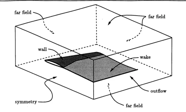
The Unsteady Full Potential equation requires that boundary conditions be applied at infinity, on the surface of the body, and on both sides of a trailing wake, as shown in Fig. 3.1. A symmetry boundary condition is applied at the wing root to reduce the size of the computational system. Symmetry is enforced by using the boundary condition for a nonmoving solid wall.

far field

Figure 3.1: Boundary Conditions

Only 2D airfoils and 3D wings cantilevered from a wall will be considered in this thesis. The 3D code is used to solve the airfoil examples by using-a straight wing set between two solid walls.

Far Field BC

The far field boundary condition is an approximation of the physical boundary condi-tion at infinity, which is necessitated by a finite computacondi-tional domain. The physical condition is that disturbances must go to zero at infinity (except directly downstream from the body, which will be treated shortly). Since the disturbances go to zero at infinity, at some finite distance they become sufficiently negligible. Thus, the boundary condition at infinity is replaced with a similar condition at a boundary far from the body. In general, this can be imposed via a Dirichlet condition

S= 4l|farfield (3.18)

the far field boundary can significantly reduce the required size of the computational domain. For instance, the wing can be modeled as a horseshoe vortex, and its associated potential at the far field boundary can be used as 1fyarfield. For the purposes of this thesis, 0lfarfield will be conveniently set to zero. This, in effect, sets the outer boundary to a uniform freestream pressure. The limitations of this choice have no major effect on the main thrust of the this work, though its effects will be seen in Chapter 5.

Outflow BC

Downstream from the body only the streamwise disturbances go to zero. This is because the Kutta condition requires a jump in q across the wake. To allow this jump a Neumann

condition is enforced at the outflow boundary

VO. utf low = 0 (3.19)

where, n is the outward pointing unit normal vector at the outflow boundary.

Wake BC

The irrotational nature of the Harmonic-Unsteady Full Potential equation requires that vorticity contained in a physical wake behind the wing be approximated as a zero-thickness vortex sheet. The sheet is then made a boundary of the system, thus allowing the interior to remain irrotational. The boundary condition applied to the wake is that the wake cannot support a pressure difference. Since viscosity is neglected there is no mechanism to shed vorticity, therefore, to set the circulation requires that an additional constraint be imposed. This constraint, the Kutta condition, is based on empirical observation and requires that the circulation be continuous at the trailing edge [25]. Computationally, this is just the wake boundary condition applied at the trailing edge of the wing.

Physically the wake deforms and rolls up at the edges to satisfy the zero pressure jump condition, so the computation should compute the geometry of the wake sheet as

part of the solution. This, unfortunately, is too computationally intensive and difficult. Instead, the wake position in thesis is set by the grid generator and has no roll up at the tips. In practice, this approximation has negligible effect on the solution for most flow situations.

The wake surface represents two boundary surfaces, so two boundary conditions need to be specified. On the upper surface the flux into the upper wake is forced to be equal to the flux out of the lower wake

(pV n), - (pV n), = 0 (3.20)

On the lower surface the zero pressure jump condition is applied

p. - p1 = 0 (3.21)

where, ( ), and ( )r indicate evaluation on the upper and lower wake surfaces, respec-tively. Substitute Eqs. (3.9) and (3.13) into Eq. (3.21) and rearrange to arrivd at the final form of the wake boundary condition

2_(u- q )+ (V - V2) = 0 (3.22)

Wall BC

The final boundary condition is imposed on the surface of the body and requires that the fluid adjacent to the body must have the same normal component of velocity as the body. The development of this boundary condition has profound ramifications for both

the analysis and the sensitivity aspects of the present code. Because of its importance this boundary condition will be explored in considerably more detail than the others.

The physical condition for the flow of an inviscid fluid around a solid body is that no flux is allowed through the walls of the body

VB T

VB = at

Figure 3.2: Wall Boundary Condition Parameters

where, n is the wall surface unit normal vector pointing into the domain (see Fig. 3.2). As explained in the previous chapter the aeroelastic equations will be solved using a Newton method. Thus, the above equation needs to be put into linearized form. For reasons that will become obvious, the wall boundary condition residual is written in functional form as

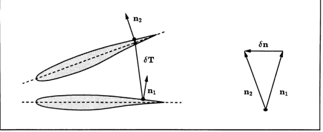
Rbs

where, T is defined in Fig. 3.2. The linearized form of this residual is

IRa \' 5 IORbc E V I R \?

R' = Rr + 0 4 + B

T)

Neither T nor n depend on the unknown, 0, so grouping all the unknowns on the left hand side and setting Rf+

i

(

6T

r 6

-

= -R

4

+ P

T) -

-

8T -

.n

(