Adaptive optimization problems under uncertainty with limited feedback

(1)

Adaptive Optimization Problems under Uncertainty with

Limited Feedback

by

Arthur Flajolet

M.S., Ecole Polytechnique (2013)

Submitted to the Sloan School of Management

in partial fulfillment of the requirements for the degree of

Doctor of Philosophy in Operations Research

at the

MASSACHUSETTS INSTITUTE OF TECHNOLOGY

June 2017

c

○ Massachusetts Institute of Technology 2017. All rights reserved.

Author . . . .

Sloan School of Management

May 15, 2017

Certified by . . . .

Patrick Jaillet

Dugald C. Jackson Professor of Electrical Engineering and Computer

Science

Thesis Supervisor

Accepted by . . . .

Dimitris Bertsimas

Boeing Professor of Operations Research

Co-director, Operations Research Center

(2)

(3)

Adaptive Optimization Problems under Uncertainty with Limited

Feedback

by

Arthur Flajolet

Submitted to the Sloan School of Management on May 15, 2017, in partial fulfillment of the

requirements for the degree of

Doctor of Philosophy in Operations Research

Abstract

This thesis is concerned with the design and analysis of new algorithms for sequential optimization problems with limited feedback on the outcomes of alternatives when the en-vironment is not perfectly known in advance and may react to past decisions. Depending on the setting, we take either a worst-case approach, which protects against a fully adver-sarial environment, or a hindsight approach, which adapts to the level of adveradver-sariality by measuring performance in terms of a quantity known as regret.

First, we study stochastic shortest path problems with a deadline imposed at the desti-nation when the objective is to minimize a risk function of the lateness. To capture distri-butional ambiguity, we assume that the arc travel times are only known through confidence intervals on some statistics and we design efficient algorithms minimizing the worst-case risk function.

Second, we study the minimax achievable regret in the online convex optimization framework when the loss function is piecewise linear. We show that the curvature of the decision maker’s decision set has a major impact on the growth rate of the minimax regret with respect to the time horizon. Specifically, the rate is always square root when the set is a polyhedron while it can be logarithmic when the set is strongly curved.

Third, we study the Bandits with Knapsacks framework, a recent extension to the standard Multi-Armed Bandit framework capturing resource consumption. We extend the methodology developed for the original problem and design algorithms with regret bounds that are logarithmic in the initial endowments of resources in several important cases that cover many practical applications such as bid optimization in online advertising auctions.

Fourth, we study more specifically the problem of repeated bidding in online adver-tising auctions when some side information (e.g. browser cookies) is available ahead of submitting a bid. Optimizing the bids is modeled as a contextual Bandits with Knapsacks problem with a continuum of arms. We design efficient algorithms with regret bounds that scale as square root of the initial budget.

(4)

(5)

Acknowledgments

First and foremost, I would like to thank my advisor Patrick Jaillet for his continued and unconditional support and guidance. Patrick is not only a brilliant mind but also a patient and caring professor who is always open to new ideas. I am very grateful for everything he has done for me and in particular for providing me with countless opportunities during my stay at MIT such as attending conferences, interning at a major demand-side platform, and collaborating with brilliant researchers at MIT and elsewhere. It has been a great honor and pleasure to work with him for the past four years.

I would also like to thank my doctoral committee members Vivek Farias and Alexander (Sasha) Rakhlin not only for their valuable feedback on my work but also for giving me the opportunity to TA for them. Vivek and Sasha are exceptional teachers and assisting them in their work has taught me alot. I have also been very fortunate to collaborate with Sasha on open problems in the field of online learning. Sasha is a phenomenal researcher as well as a wonderful person and I have learned a great deal about online learning working with him. I would also like to thank Laura Rose and Andrew Carvalho for all their help over the years.

My PhD would not have been the same without all the great people I met here, start-ing with my roommates (past and present): Andrew L., Mathieu D., Zach O., Virgile G., Maxime C., and Florent B.. I am grateful for all the good times we have had together. I would also like to make a special mention of the worthy members of the sushi squad: Charles T., Anna P., Sebastien M., Joey H., Max Burq, Max Biggs, Stefano T., Zach S., Colin P., and Elisabeth P.. May the team live on forever. I would also like to thank all the friends I met at MIT and especially: Ludovica R., Cecile C., Sebastien B., Ali A., Anne C., Audren C., Elise D., Rim H., Ilias Z., Alex R., Alex S., Alex B., Rachid N., Alexis T., Pierre B., Maher D., Velibor M., Nishanth M., Mariapaola T., Zeb H., Dan S., Will M., Antoine D., Jean P., Jonathan A., Arthur D., Konstantina M., Nikita K., Chong Yang G., Jehangir A., Swati G., Rajan U., Clark P., and Eli G..

I would also like to thank S. Hunter in a separate paragraph because he has been such a great friend.

(6)

Finally, I would like to acknowledge my family, particularly my mother and my father, who have always been there for me. I would not be here if it was not for them.

This research was supported by the National Research Foundation Grant No. 015824-00078 and the Office of Naval Research Grant N00014-15-1-2083.

(7)

List of Figures

2-1 Existence of loops in adaptive stochastic shortest path problems . . . 34

2-2 Existence of infinite cycling from Example 2.1 . . . 35

2-3 Graph of 𝑢Δ𝑡_𝑗 (·) . . . 57

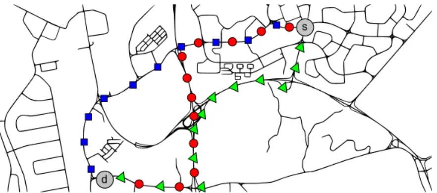
2-4 Local map of the Singapore road network . . . 59

2-5 Average computation time as a function of the time budget for 𝜆 = 0.001 . 62 2-6 Performance for 𝜆 = 0.001, average number of samples per link: ∼ 5.5 . . 62

2-7 Performance for 𝜆 = 0.002, average number of samples per link: ∼ 9.4 . . 63

(12)

(13)

List of Tables

2.1 Literature review of stochastic shortest path problems . . . 28 2.2 Routing methods considered . . . 61 3.1 Growth rate of 𝑅𝑇 in several settings of interest . . . 72

(14)

(15)

Chapter 1 Introduction

1.1 Motivation and General Setting

In many practical applications, the decision making process is fundamentally sequential and takes place in an uncertain, possibly adversarial, environment that is too complex to be fully comprehended. As a result, planning can no longer be regarded as a one-shot proce-dure, where the entire plan would be laid out ahead of time, but rather as a trial-and-error process, where the decision maker can assess the quality of past actions, adapt to new cir-cumstances, and potentially learn about the surrounding environment. Arguably, we face many such problems in our daily life. Routing vehicles in transportation networks is a good example since traffic conditions are constantly evolving according to dynamics that are dif-ficult to predict. As drivers, we have little control over this exogenous parameter but we are nevertheless free to modify our itinerary at any point in time based on the latest available traffic information. In this particular application, the environment is not cooperative but also not necessarily adversarial. There are, however, other settings, such as dynamic pric-ing in the airline industry, where the environment is clearly pursupric-ing a conflictpric-ing goal. In this last setting, the ticket agent dynamically adjusts prices as a function of the remaining inventory, the selling horizon, and the perceived willingness to pay while potential cus-tomers act strategically in order to drive the prices down.

At an abstract level, we consider the following class of sequential optimization prob-lems. At each stage, the decision maker first selects an action out of a set of options, whose

(16)

availability depend on the decision maker’s current state, based on the information acquired in the past. Next, the environment, defined as everything outside of the decision maker’s control (e.g. traffic conditions in the vehicle routing routing application mentioned above), transitions into a new state, possibly in reaction to this choice. Finally, the decision maker transitions into a new state, obtains a scalar reward, and receives some feedback on the outcomes of alternatives as a function of not only the action that was implemented but also the new state of the environment. We then move onto the next stage and this process is repeated until the decision maker reaches a terminal state. His or her goal is to maximize some prescribed objective function of the sum of the rewards earned along the way. The specificity of the sequential optimization problems studied in this thesis lies in two key features:

1. the environment is uncertain. The decision maker knows which states the environ-ment might occupy but he or she has little a priori knowledge on its internal mechan-ics: its initial state, its transition rules from one state to another, and its objectives; 2. the feedback received at each stage is very limited. As a result, the decision maker

can never perform a thorough counterfactual analysis, which limits his or her ability to learn from past mistakes.

In the above description, uncertainty is not used as a placeholder for stochasticity. Stochas-ticity can be a source of uncertainty but it need not be the only one or the most important one. For instance, even when the environment is governed by a stochastic process, the underlying distributions might be a priori unknown as in Chapter 2. Going further, stochas-ticity may not even be involved in the modeling. This is the case, for example, when the problem is to optimize an unknown deterministic function 𝑓 (·), lying in a known set of general functions, by making repeated value queries.

As the environment is uncertain, the optimization problem faced by the decision maker is ill-defined since merely computing the objective function requires knowing the sequence of states occupied by the environment. In Section 1.2, we detail two possible approaches: a worst-case approach, that protects the decision maker against a fully adversarial envi-ronment, and a hindsight approach, that adapts to the level of adversariality at the price of

(17)

deriving a suboptimal objective function if the environment happens to be fully adversarial. In the next four chapters, depending on the setting, we study one of these approaches with an emphasis on computational tractability and performance analysis. A precise overview of contributions is given in Section 1.3.

The framework considered in this thesis is, in many respects, strongly reminiscent of Reinforcement Learning (RL) but the focus is different. In RL, the environment is often governed by a stochastic process that the decision maker can learn from through repeated interaction. Since there is limited feedback on the outcome of alternatives, this naturally gives rise to an exploration-exploitation trade-off. In this thesis, the focus is on optimization as opposed to learning and we substitute the concept of uncertainty for that of stochasticity. As a consequence, there might be nothing to learn from for the decision maker in general, as in Chapters 2 and 3, but he or she might need to learn something about the environment in order to perform well, as in Chapters 4 and 5. Note that this is merely a choice of focus and this does not imply by any means that there are no connections to learning. Learn-ing and optimization are intrinsically tied topics whose frontiers are becomLearn-ing increasLearn-ingly blurred. However, taking a pure optimization standpoint, abstracting away learning con-siderations, has proved particularly successful in the RL literature. A good example of this trend is given by the growing popularity of the online convex optimization framework, studied in Chapter 3 and originally developed by the machine learning community, which has led to significant advances in RL. As a recent illustration, the authors of [80] show that establishing martingale tail bounds is essentially equivalent to solving online convex optimization problems. Given that concentration inequalities are intrinsic to any kind of learning, this constitutes a clear step towards bringing together optimization and learning theory. Connections between optimization and learning theory will also appear throughout this thesis.

1.2 Mathematical Framework

In this section, we sketch the common mathematical framework underlying the problems studied in this thesis. For the purpose of describing it at a high level in a mathematically

(18)

precise way, we need to introduce notations that may differ from the ones used in later chapters.

Stages are discrete and indexed by 𝑡 ∈ N. At the beginning of stage 𝑡, the environment (resp. the decision maker) is in state 𝑒𝑡 ∈ 𝐸 (resp. 𝑠𝑡 ∈ 𝑆). The set of actions available to

the decision maker in state 𝑠 ∈ 𝑆 is denoted by 𝐴(𝑠). At stage 𝑡, the decision maker takes an action 𝑎𝑡 ∈ 𝐴(𝑠𝑡), from which he or she derives a scalar reward 𝑟𝑡 and receives some

feedback on the outcomes of alternatives in the form of a multidimensional vector 𝑜𝑡. The

decision made at stage 𝑡 can be based upon all the information acquired in the past, namely ((𝑠𝜏, 𝑎𝜏, 𝑟𝜏, 𝑜𝜏))𝜏 ≤𝑡−1along with 𝑠𝑡, which we symbolically denote by ℱ𝑡. To select these

actions, the decision maker uses an algorithm 𝒜 in A, a subset of all non-anticipating al-gorithms that, at any stage 𝑡, map ℱ𝑡to a (possibly randomized) action in 𝐴(𝑠𝑡). Similarly,

the environment uses a decision rule 𝒟 in D, a subset of all non-anticipating decision rules that, at any stage 𝑡, map the information available to it, namely ((𝑠𝜏, 𝑎𝜏, 𝑟𝜏, 𝑜𝜏, 𝑒𝜏))𝜏 ≤𝑡−1

along with 𝑠𝑡and 𝑎𝑡, to a (possibly randomized) state 𝑒𝑡+1 ∈ 𝐸. In addition, 𝒟 determines

the initial state of the environment ahead of stage 1. The reward and feedback provided to the decision maker at the end of stage 𝑡 are determined by prescribed (possibly stochastic) rules outside of the environment’s control. The sequential process ends at stage 𝜏* when the decision maker reaches a terminal stage. In many settings, there is a deterministic time horizon 𝑇 , in which case 𝜏* = 𝑇 . Given a prescribed scalar function 𝜑(·), the goal for the decision maker is to maximize the objective function 𝜑(∑︀𝜏*

𝑡=1𝑟𝑡), which we denote by

obj(𝒜, 𝒟) to underline the fact that it is determined by a deep interplay between 𝒜 and 𝒟. The exact expression of 𝜑(·) may be complex and involve expectations. In fact, even when the environment is deterministic and perfectly known in advance, maximizing the objective function can be a difficult computational problem.

Since 𝒟 is a priori unknown, maximizing obj(𝒜, 𝒟) over 𝒜 in A is an ill-defined op-timization problem. To remove any ambiguity, a natural approach is to infer 𝒟 based on the initial knowledge and to take it as an input. However, this approach is not ro-bust in the sense that there are no guarantees on the performance of the optimal solution to max_𝒜∈Aobj(𝒜, 𝒟) if 𝒟 happens to deviate from what was inferred, even if only so slightly. This is particularly problematic if the decision maker expects the environment to

(19)

be governed by a stochastic process while it is, in fact, adversarial. A variety of robust ap-proaches have been developed in the literature, each with its own optimization formulation that comes with provable guarantees on the performance of the solution derived. In this thesis, we focus on two approaches that do not require additional modeling assumptions about the environment: the worst-case approach and the hindsight approach. This effec-tively rules out the Bayesian optimization approach which requires some prior knowledge on 𝒟 in the form of a distribution on D, in which case the performance guarantees are mea-sured in terms of this prior. Ideally, the decision maker should pick an approach based on whether it is critical to be prepared for the worst-case scenario for the particular application at hand. However, in many cases, computational tractability and ease of analysis end up being the main criteria.

1.2.1 Worst-Case Approach

In this approach, the decision maker protects himself or herself against the worst-case sce-nario of facing a fully adversarial environment and solves:

max

𝒜∈A min𝒟∈Dobj(𝒜, 𝒟). (1.1)

Denote by 𝒜* an optimal solution to (1.1). By construction, the objective function derived

from 𝒜*is always at least no smaller than the optimal value of (1.1), irrespective of which decision rule 𝒟 in D is used by the environment. The main drawback of this approach is that, depending on 𝒟, the objective function may be much larger than the optimal value of (1.1) but no better guarantees can be derived. Note that, depending on the modeling, a worst-case analysis is not necessarily over-conservative since D may be a small set.

1.2.2 Hindsight Approach

In this approach, the goal is to adapt to the level of adversariality of the environment by comparing, uniformly over all 𝒟 ∈ D, the objective function derived by the decision maker with the largest one he or she could have obtained in hindsight, i.e. if 𝒟 was initially

(20)

known. Several comparison metrics have been proposed in the literature.

Regret metric. When the comparison is done by means of a subtraction, the metric of interest is called regret, often mathematically defined as:

ℛ(𝒜) = max

𝒟∈D {max_{𝒜∈ ˜}˜ _Aobj( ˜𝒜, 𝒟) − obj(𝒜, 𝒟)}, (1.2)

for 𝒜 ∈ A and where ˜A is a subclass of non-anticipating algorithms that may be different from A. The computational problem faced by the decision maker is to find an efficient algorithm 𝒜 that, at least approximately, minimizes ℛ(𝒜). If min_𝒜∈Aℛ(𝒜) is small, the decision maker performs almost as well as if he or she had initially been provided with 𝒟, as shown by the inequality:

obj(𝒜, 𝒟) ≥ max

˜

𝒜∈ ˜_Aobj( ˜𝒜, 𝒟) − ℛ(𝒜) (1.3)

that holds for every 𝒜 ∈ A irrespective of which decision rule 𝒟 in D is used by the envi-ronment.

There are many alternative definitions of regret that vary slightly from (1.2). In many frameworks, such as in online convex optimization, the benchmark max_{𝒜∈ ˜}˜ _Aobj( ˜𝒜, 𝒟)

dif-fers along two lines. First, ˜𝒜 is not facing the same decision rule 𝒟 as 𝒜: the environment is assumed to follow a state path identical to the one that would have been followed if the decision maker had implemented 𝒜, as opposed to reacting to the actions dictated by ˜𝒜 (which would lead to a different path). Second, ˜_{A is a subclass of all-knowing algorithms} that are initially provided with the state path followed by the environment. Thus, in stark contrast with frameworks that use (1.2) as a definition for regret, such as stochastic multi-armed bandit problems, the benchmark is not necessarily physically-realizable in online convex optimization. This is a critical difference that is motivated by technical consider-ations: the framework is completely model-free, i.e. D is the set of all non-anticipating decision rules, and, as a result, it is usually impossible to get non-trivial bounds on (1.2). This change in definition makes it possible to establish non-trivial regret bounds while still encompassing many settings of interest, such as the the standard i.i.d. statistical learning

(21)

framework, see the discussion below. For the purpose of simplifying the presentation, we keep the notations unchanged but they could easily be adapted to include these frameworks. A new idea that has received considerable attention in the recent years is to derive regret bounds that also adapt to the level of adversariality of the environment, see, for example, [79] and [47]. In this line of work, the goal is to find an algorithm 𝒜 ∈ A as well as a function 𝑓 (·) such that:

max

𝒟∈D{max𝒜∈ ˜˜ _A

obj( ˜𝒜, 𝒟) − obj(𝒜, 𝒟) − 𝑓 (𝑒1, · · · , 𝑒𝜏*)} ≤ 0

and such that 𝑓 (𝑒1, · · · , 𝑒𝜏*) is small when the environment is not fully adversarial (e.g. slow-varying). This approach is particularly attractive when A is very large and it is im-possible to establish non-trivial bounds on min_𝒜∈Aℛ(𝐴).

Researchers also now distinguish various notions of regret based on the exact definition of ˜_{A, some of which turn out to be closely related, see, for example, [26]. For instance, in} the online convex optimization framework, researchers distinguish the concept of dynamic regret, when ˜_{A is the set of all unconstrained all-knowing algorithms, from that of (static)} external regret, when ˜A is restricted to all-knowing algorithms that are constrained to select the same action across stages. This last notion is motivated by the standard statistical learn-ing settlearn-ing: if the environment happens to be governed by an i.d.d. stochastic process then bounds on the external regret directly translate into oracle inequalities. Since the minimal external regret can often be shown to be identical, up to constant factors, to the optimal statistical learning rate and since many efficient algorithms have been designed to achieve near-optimal regret, we get optimal statistical learning rates “for free”, i.e. without ever assuming that the environment is governed by a stochastic process.

Competitive ratio metric. When 𝜑(·) is a positive function, the comparison can done by means of a ratio, in which case the metric of interest is called competitive ratio, often mathematically defined as:

𝒞(𝒜) = min

𝒟∈D

obj(𝒜, 𝒟) max𝒜∈ ˜˜ _Aobj( ˜𝒜, 𝒟)

(22)

where ˜_{A is a subclass of non-anticipating algorithms that may be different from A.} Sim-ilarly as for the regret metric, the computational problem faced by the decision maker is then to find an efficient algorithm 𝒜 that, at least approximately, minimizes 𝒞(𝒜). The resulting performance guarantee is:

obj(𝒜, 𝒟) ≥ 𝒞(𝒜) · max

˜ 𝒜∈ ˜_A

obj( ˜𝒜, 𝒟) (1.5)

and holds for every 𝒜 ∈ A irrespective of which decision rule 𝒟 in D is used by the environment.

Just like for the regret metric, a number of variants have been proposed in the literature where the exact definition of the competitive ratio may vary slightly from (1.4) and ˜A is typically a subset of all-knowing algorithms. Since the competitive ratio metric will not be the metric of choice in this thesis, we refer to the literature for a more thorough introduction to competitive analysis, see in particular [28] and [59].

Comparison of metrics. Regret and competitive ratio metrics are known to be incom-parable and, in general, incompatible, see [10]. For this reason, the choice is often based on technical considerations, such as whether the metric lends itself well to analysis, which heavily depends on the framework. Competitive analysis is usually well suited for prob-lems where, at each stage, the decision maker receives some information on the state of the environment before selecting an action while regret metrics tend to facilitate the analysis in Bayesian settings by linearity of expectation.

1.3 Overview of Thesis

In Chapter 2, we study a vehicle routing problem and take a worst-case approach for which we design efficient algorithms. Chapters 3, 4, and 5 are all dedicated to the hindsight approach. In Chapter 3, we establish a thorough characterization of the minimax achievable regret in online convex optimization when the loss function is piecewise linear. In Chapters 4 and 5, we design efficient algorithms with provable near-optimal regret for Bandits with Knapsacks problems, an extension of Multi-Armed Bandit problems capturing resource

(23)

consumption, with a particular emphasis on applications in the online advertising industry. Each chapter is summarized in more detail in the remainder of this section.

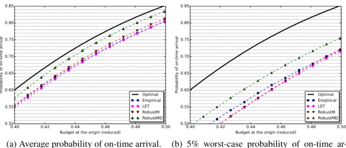
Robust Adaptive Routing under Uncertainty. We consider the problem of finding an optimal history-dependent routing strategy on a directed graph weighted by stochastic arc costs when the objective is to minimize the risk of spending more than a prescribed budget. To help mitigate the impact of the lack of information on the arc cost probability distribu-tions, we introduce a worst-case robust counterpart where the distributions are only known through confidence intervals on some statistics such as the mean, the mean absolute devia-tion, and any quantile. Leveraging recent results in distributionally robust optimizadevia-tion, we develop a general-purpose algorithm to compute an approximate optimal strategy. To il-lustrate the benefits of the worst-case robust approach, we run numerical experiments with field data from the Singapore road network.

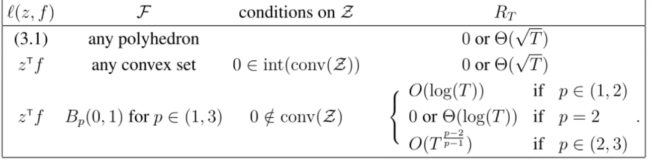
No-Regret Learnability for Piecewise Linear Losses. In the convex optimization ap-proach to online regret minimization, many methods have been developed to guarantee a

𝑂(√𝑇 ) bound on regret for linear loss functions. These results carry over to general convex

loss functions by a standard reduction to linear ones. This seems to suggest that linear loss functions are the hardest ones to learn against. We investigate this question in a systematic fashion looking at the interplay between the set of possible moves for both the decision maker and the adversarial environment. This allows us to highlight sharp distinctive be-haviors about the learnability of piecewise linear loss functions. On the one hand, when the decision set of the decision maker is a polyhedron, we establish Ω(√𝑇 ) lower bounds

on regret for a large class of piecewise linear loss functions with important applications in online linear optimization, repeated Stackelberg games, and online prediction with side information. On the other hand, we exhibit 𝑜(√𝑇 ) learning rates, achieved by the

Follow-The-Leader algorithm, in online linear optimization when the decision maker’s decision set is curved and when 0 does not lie in the convex hull of the environment’s decision set. Hence, the curvature of the decision maker’s decision set is a determining factor for the optimal rate.

(24)

Logarithmic Regret Bounds for Bandits with Knapsacks. Optimal regret bounds for Multi-Armed Bandit problems are now well documented. They can be classified into two categories based on the growth rate with respect to the time horizon 𝑇 : (i) small, dependent, bounds of order of magnitude ln(𝑇 ) and (ii) robust, distribution-free, bounds of order of magnitude √𝑇 . The Bandits with Knapsacks model, an

exten-sion to the framework allowing to model resource consumption, lacks this clear-cut dis-tinction. While several algorithms have been shown to achieve asymptotically optimal distribution-free bounds on regret, there has been little progress toward the development of small distribution-dependent regret bounds. We partially bridge the gap by designing a general-purpose algorithm with distribution-dependent regret bounds that are logarithmic in the initial endowments of resources in several important cases that cover many practi-cal applications, including dynamic pricing with limited supply, bid optimization in online advertisement auctions, and dynamic procurement.

Real-Time Bidding with Side Information. We consider the problem of repeated bid-ding in online advertising auctions when some side information (e.g. browser cookies) is available ahead of submitting a bid in the form of a 𝑑-dimensional vector. The goal for the advertiser is to maximize the total utility (e.g. the total number of clicks) derived from displaying ads given that a limited budget 𝐵 is allocated for a given time horizon 𝑇 . Op-timizing the bids is modeled as a linear contextual Multi-Armed Bandit (MAB) problem with a knapsack constraint and a continuum of arms. We develop UCB-type algorithms that combine two streams of literature: the confidence-set approach to linear contextual MABs and the probabilistic bisection search method for stochastic root-finding. Under mild as-sumptions on the underlying unknown distribution, we establish distribution-independent regret bounds of order ˜𝑂(𝑑 ·√𝑇 ) when either 𝐵 = ∞ or when 𝐵 scales linearly with 𝑇 .

(25)

Chapter 2 Robust Adaptive Routing under

Uncertainty

2.1 Introduction

2.1.1 Motivation

Stochastic Shortest Path (SSP) problems have emerged as natural extensions to the classi-cal shortest path problem when arc costs are uncertain and modeled as outcomes of random variables. In particular, we consider in this chapter the class of adaptive SSPs, which can be formulated as Markov Decision Processes (MDPs), where we optimize over all history-dependent strategies. As standard with MDPs, optimal policies are characterized by dy-namic programming equations involving expected values (e.g. [22]). Yet, computing the expected value of a function of a random variable generally requires a full description of its probability distribution, and this can be hard to obtain accurately due to errors and spar-sity of measurements. In practice, only finite samples are available and an optimal strategy based on approximated arc cost probability distributions may be suboptimal with respect to the real arc cost probability distributions.

In recent years, Distributionally Robust Optimization (DRO) has emerged as a new framework for decision-making under uncertainty when the underlying distributions are only known through some statistics or from collections of samples. DRO was put forth in

(26)

an effort to capture both risk (uncertainty on the outcomes) and ambiguity (uncertainty on the probabilities of the outcomes) when optimizing over a set of alternatives. The com-putational complexity of this approach can vary greatly, depending on the nature of the ambiguity sets and on the structure of the optimization problem, see [100] and [38] for convex problems, and [31] for chance-constraint problems. Even in the absence of deci-sion variables, the theory proves useful to derive either numerical or closed form bounds on expected values using optimization tools, see, for example, [77], [23], and [94].

In the case of limited knowledge of the arc cost probability distributions, we propose to bring DRO to bear on adaptive SSP problems to help mitigate the impact of the lack of information. Our work fits into the literature on Distributionally Robust MDPs (DRMDPs) where the transition probabilities are only known to lie in prescribed ambiguity sets (e.g. [69], [104], and [99]). While the methods developed in the aforementioned literature carry over, adaptive SSPs exhibit a particular structure that allows for a large variety of ambi-guity sets and enables the development of faster solution procedures. Specifically, optimal strategies for DRMDPs are characterized by a Bellman recursion on the worst-case ex-pected reward-to-go. While standard approaches focus on computing this quantity for each state independently from one another, closely related problems (e.g. estimating an expected value E[𝑓 (𝑡 − 𝑋)] where the random variable 𝑋 is fixed but 𝑡 varies across states) carry across states for adaptive SSPs. As a result, making the most of previous computations becomes crucial for computational tractability. This entails keeping track of the extreme points of a dynamically changing set efficiently, revealing an interesting connection be-tween DRMDPs and Dynamic Convex Hull problems.

2.1.2 Related Work and Contributions

Over the years, many SSP problems have been formulated. They differ along three main features:

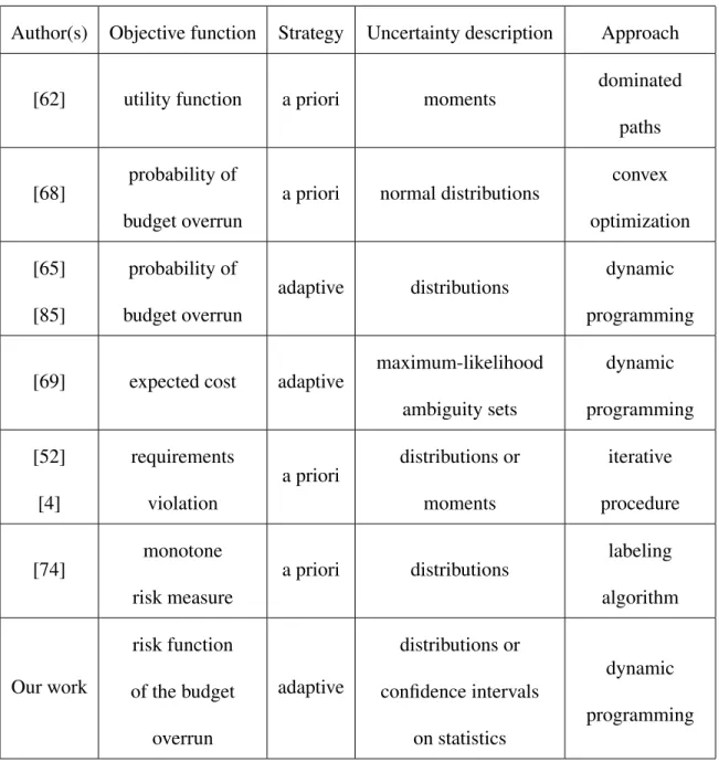
∙ The specific objective function to optimize: in the presence of uncertainty, minimiz-ing the expected costs is a natural approach, see [22], but it is oblivious to risk. [62] proposed earlier to rely on utility functions of statistical moments involving an

(27)

inher-ent trade-off, and considered multi-objective criteria. However, Bellman’s principle of optimality no longer holds in this case, giving rise to computational hardness. A different approach consists of (1) introducing a budget, set by the user, correspond-ing to the maximum cost he is willcorrespond-ing to pay to reach his terminal node and (2) minimizing either the probability of budget overrun (see [41], [68], and also [105] for probabilistic goal MDPs), more general functions of the budget overrun as in [67], satisficing measures to guarantee good performances with respect to multiple objectives as in [52], or the expected costs while also constraining the probability of budget overrun as in [103].

∙ The set of strategies over which we are free to optimize: incorporating uncertainty may cause history-dependent strategies to significantly outperform a priori paths de-pending on the performance index. This is the case when the objective is to maximize the probability of completion within budget for which two types of formulations have been considered: (i) an a priori formulation which consists of finding a path before taking any actions, see [68] and [66]; and (ii) an adaptive formulation which allows to update the path to go based on the remaining budget, see [65] and [85].

∙ The knowledge on the random arc costs taken as an input: it can range from the full knowledge of the probability distributions to having access to only a few samples drawn from them. In practical settings, the problem of estimating some statistics seems more reasonable than retrieving the full probability distribution. For instance, [52] consider lower-order statistics (minimum, average, and maximum costs) and use closed form bounds derived in the DRO theory. These considerations were ex-tensively investigated in the context of DRMDPs, see [51] and [99] for theoretical developments. The ambiguity sets are parametric in [99], where the parameter lies in the intersection of ellipsoids, are based on likelihood measures in [69], and are defined by linear inequalities in [98].

(28)

Table 2.1: Literature review of stochastic shortest path problems.

Author(s) Objective function Strategy Uncertainty description Approach

[62] utility function a priori moments

dominated paths

[68]

probability of budget overrun

a priori normal distributions

convex optimization [65] [85] probability of budget overrun adaptive distributions dynamic programming

[69] expected cost adaptive

maximum-likelihood ambiguity sets dynamic programming [52] [4] requirements violation a priori distributions or moments iterative procedure [74] monotone risk measure a priori distributions labeling algorithm Our work risk function of the budget overrun adaptive distributions or confidence intervals on statistics dynamic programming

(29)

Contributions. The main contributions of this chapter can be summarized as follows: 1. We extend the class of adaptive SSP problems to general risk functions of the budget

overrun and to the presence of distributional ambiguity.

2. We characterize optimal strategies and identify conditions on the risk function under which infinite cycling is provably suboptimal.

3. For any risk function satisfying these conditions, we provide efficient solution proce-dures (invoking fast Fourier transforms and dynamic convex hull algorithms as sub-routines) to compute 𝜖-approximate optimal strategies when the arc cost distributions are either exactly known or only known through confidence intervals on piecewise affine statistics (e.g. the mean, the mean absolute deviation, any quantile...) for any

𝜖 > 0.

Special cases where (i) the objective is to minimize the probability of budget overrun and (ii) the arc costs are independent discrete random variables can serve as a basis for com-parison with prior work on DRMDPs. For this subclass of problems, our formulation can be interpreted as a DRMDP with finite horizon 𝑁 , finitely many states 𝑛 (resp. actions 𝑚), and a rectangular ambiguity set. Our methodology can be used to compute an 𝜖-optimal strategy with complexity 𝑂(𝑚 · 𝑛 · log(𝑁_𝜖) · log(𝑛)).

The remainder of the chapter is organized as follows. In Section 2.2, we introduce the adaptive SSP problem and its distributionally robust counterpart. Section 2.3 (resp. Section 2.4) is devoted to the theoretical and computational analysis of the nominal (resp. robust) problem. In Section 2.5, we consider a vehicle routing application and present results of numerical experiments run with field data from the Singapore road network. In Section 2.6, we relax some of the assumptions made in Section 2.2 and extend the results presented in Sections 2.3 and 2.4.

Notations. For a function 𝑔(·) and a random variable 𝑋 distributed according to 𝑝, we denote the expected value of 𝑔(𝑋) by E𝑋∼𝑝[𝑔(𝑋)]. For a set 𝑆 ⊂ R𝑛, ¯𝑆 is the closure of 𝑆

(30)

For a set 𝑆 ⊂ R2, ^𝑆 denotes the upper convex hull of 𝑆, i.e. ^_{𝑆 = {(𝑥, 𝑦) ∈ R}2 _{: ∃(𝑎, 𝑏) ∈}

conv(𝑆) such that 𝑥 = 𝑎 and 𝑦 ≥ 𝑏}.

2.2 Problem Formulation

2.2.1 Nominal Problem

Let 𝒢 = (𝒱, 𝒜) be a finite directed graph where each arc (𝑖, 𝑗) ∈ 𝒜 is assigned a collection of non-negative random costs (𝑐𝜏

𝑖𝑗)𝜏 ≥0. We consider a user traveling through 𝒢 leaving from

𝑠 and wishing to reach 𝑑 within a prescribed budget 𝑇 . Having already spent a budget 𝜏

and being at node 𝑖, choosing to cross arc (𝑖, 𝑗) would incur an additional cost 𝑐𝜏

𝑖𝑗, whose

value becomes known after the arc is crossed. In vehicle routing applications, 𝑐𝜏_𝑖𝑗 typically models the travel time along arc (𝑖, 𝑗) at time 𝜏 and 𝑇 is the deadline imposed at the destination. The objective is to find a strategy to reach 𝑑 maximizing a risk function of the budget overrun, denoted by 𝑓 (·). Mathematically, this corresponds to solving:

sup

𝜋∈ΠE[𝑓 (𝑇 − 𝑋

𝜋)], (2.1)

where Π is the set of all history-dependent randomized strategies and 𝑋𝜋 is the random

cost associated with strategy 𝜋 when leaving from node 𝑠 with budget 𝑇 . Examples of natural risk functions include 𝑓 (𝑡) = 𝑡 · 1𝑡≤0, 𝑓 (𝑡) = 1𝑡≥0, and 𝑓 (𝑡) = −|𝑡| which translate

into, respectively, minimizing the expected budget overrun, maximizing the probability of completion within budget, and penalizing the expected deviation from the target budget. We will restrict our attention to risk functions satisfying natural properties meant to prevent infinite cycling in Theorem 2.1 of Section 2.3.1, e.g. maximizing the expected budget overrun is not allowed. Without any additional assumption on the random costs, (2.1) is computationally intractable. To simplify the problem, a common approach in the literature is to assume independence of the arc costs, see for example [40].

Assumption 2.1. (𝑐𝜏_𝑖𝑗)(𝑖,𝑗)∈𝒜,𝜏 ≥0are independent random variables.

(31)

and Assumption 2.1 may then appear unreasonable. Most of the results derived in this chapter can be extended when the experienced costs are modeled as a Markov chain of finite order. To simplify the presentation, Assumption 2.1 is used throughout the chapter and this extension is discussed in Section 2.6.1. For the same reason, the arc costs are also assumed to be identically distributed across 𝜏 .

Assumption 2.2. For all arcs (𝑖, 𝑗) ∈ 𝒜, the distribution of 𝑐𝜏

𝑖𝑗 does not depend on𝜏 .

The extension to 𝜏 -dependent arc cost distributions is detailed in Section 2.6.2. For clarity of the exposition, we omit the superscript 𝜏 when it is unnecessary and simply denote the costs by (𝑐𝑖𝑗)(𝑖,𝑗)∈𝒜, even though the cost of an arc corresponds to an independent

realization of its corresponding random variable each time it is crossed. Motivated by computational and theoretical considerations that will become apparent in Section 2.3.2.b, we further assume that the arc cost distributions have compact supports throughout the chapter. This assumption is crucial for the analysis carried out in this chapter but is also perfectly reasonable in many practical settings, such as in transportation networks.

Assumption 2.3. For all arcs (𝑖, 𝑗) ∈ 𝒜, the distribution of 𝑐𝑖𝑗, denoted by𝑝ij, has compact

support included in[𝛿inf

𝑖𝑗 , 𝛿

sup

𝑖𝑗 ] with 𝛿𝑖𝑗inf > 0 and 𝛿

sup

𝑖𝑗 < ∞. Thus 𝛿inf = min

(𝑖,𝑗)∈𝒜𝛿 inf 𝑖𝑗 > 0 and 𝛿sup = max (𝑖,𝑗)∈𝒜𝛿 sup 𝑖𝑗 < ∞.

2.2.2 Distributionally Robust Problem

A major limitation of the approach described above is that it requires a full description of the uncertainty, i.e. having access to the arc cost probability distributions. Yet, in practice, we often only have access to a limited number of realizations of the random variables 𝑐𝑖𝑗.

It is then tempting to estimate empirical arc cost distributions and to take them as input to problem (2.1). However, estimating accurately a distribution usually requires a large sample size, and our experimental evidence suggests that, as a result, the corresponding solutions may perform poorly when only a few samples are available, as we will see in Section 2.5. To address this limitation, we adopt a distributionally robust approach where, for each arc (𝑖, 𝑗) ∈ 𝒜, 𝑝𝑖𝑗 is only assumed to lie in an ambiguity set 𝒫𝑖𝑗. We make the

(32)

Assumption 2.4. For all arcs (𝑖, 𝑗) ∈ 𝒜, 𝒫𝑖𝑗 is not empty, closed for the weak topology,

and a subset of𝒫([𝛿inf

𝑖𝑗 , 𝛿

sup

𝑖𝑗 ]), the set of probability measures on [𝛿𝑖𝑗inf, 𝛿

sup

𝑖𝑗 ].

Assumption 2.4 is a natural extension of Assumption 2.3, and is essential for computational tractability, see Section 2.4. The robust counterpart of (2.1) for an ambiguity-averse user is then given by:

sup

𝜋∈Π

inf

∀(𝑖,𝑗)∈𝒜, 𝑝𝑖𝑗∈𝒫𝑖𝑗

Ep[𝑓 (𝑇 − 𝑋𝜋)], (2.2)

where the notation p refers to the fact that the costs (𝑐𝑖𝑗)(𝑖,𝑗)∈𝒜 are independent and

dis-tributed according to (𝑝𝑖𝑗)(𝑖,𝑗)∈𝒜. As a byproduct of the results obtained for the nominal

problem in Section 2.3.1, (2.2) can be equivalently viewed as a distributionally robust MDP in the extended space state (𝑖, 𝜏 ) ∈ 𝒱 × R+where 𝑖 is the current location and 𝜏 is the total

cost spent so far and where the transition probabilities from any state (𝑖, 𝜏 ) to any state (𝑗, 𝜏′), for 𝑗 ∈ 𝒱(𝑖) and 𝜏′ ≥ 𝜏 , are only known to jointly lie in a global ambiguity set. As shown in [99], the tractability of a distributionally robust MDP hinges on the decompos-ability of the global ambiguity set as a Cartesian product over the space state of individual ambiguity sets, a property coined as rectangularity. While the global ambiguity set of (2.2) is rectangular with respect to our original state space 𝒱, it is not with respect to the extended space space 𝒱 × R+. Thus, we are led to enlarge our ambiguity set to make it rectangular

and consider a conservative approximation of (2.2). This boils down to allowing the arc cost distributions to vary in their respective ambiguity sets as a function of 𝜏 . This approach leads to the following formulation:

sup 𝜋∈Π inf ∀𝜏,∀(𝑖,𝑗)∈𝒜, 𝑝𝜏 𝑖𝑗∈𝒫𝑖𝑗 Ep𝜏[𝑓 (𝑇 − 𝑋_𝜋)], (2.3)

where the notation p𝜏 refers to the fact that, for any arc (𝑖, 𝑗) ∈ 𝒜, the costs (𝑐𝜏_𝑖𝑗)𝜏 ≥0

are independent and distributed according to (𝑝𝜏

𝑖𝑗)𝜏 ≥0. Note that when Assumption 2.2 is

relaxed, we have a different ambiguity set 𝒫_𝑖𝑗𝜏 for each pair ((𝑖, 𝑗), 𝜏 ) ∈ 𝒜 × R+and (2.3)

is precisely the robust counterpart of (2.1) as opposed to a conservative approximation, see Section 2.6.2. Also observe that (2.3) reduces to (2.1) when the ambiguity sets are singletons, i.e. 𝒫𝑖𝑗 = {𝑝𝑖𝑗}. In the sequel, we focus on (2.3), which we refer to as the robust

(33)

with respect to the optimization problem (2.2) from a theoretical (resp. practical) standpoint in Section 2.4.2 (resp. Section 2.5). Finally note that we consider general ambiguity sets satisfying Assumption 2.4 when we study the theoretical properties of (2.3). However, for tractability purposes, the solution procedure that we develop in Section 2.4.3.c only applies to ambiguity sets defined by confidence intervals on piecewise affine statistics, such as the mean, the absolute mean deviation, or any quantile. We refer to Section 2.4.3.b for a discussion on the modeling power of these ambiguity sets. Similarly as for the nominal problem, we will also restrict our attention to risk functions satisfying natural properties meant to prevent infinite cycling in Theorem 2.2 of Section 2.4.1.

2.3 Theoretical and Computational Analysis of the

Nomi-nal Problem

2.3.1 Characterization of Optimal Policies

Perhaps the most important property of (2.1) is that Bellman’s Principle of Optimality can be shown to hold irrespective of the choice of the risk function. Specifically, for any history of the previously experienced costs and previously visited nodes, an optimal strategy to (2.1) must also be an optimal strategy to the subproblem of minimizing the risk function given this history. Otherwise, we could modify this strategy for this particular history and take it to be an optimal strategy for this subproblem. This operation could only increase the objective function of the optimization problem (2.1), which would contradict the optimality of the strategy.

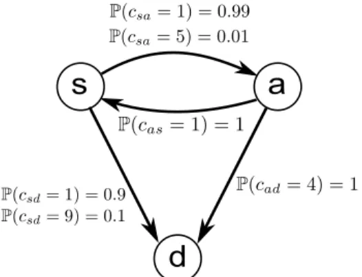
Another, less obvious, interesting feature of (2.1) is that, even for perfectly natural risk functions 𝑓 (·), making decisions according to an optimal strategy may lead to cycle back to a previously visited location. This may happen, for instance, when the objective is to maximize the probability of completion within budget, see [85], and their example can be adapted when the objective is to minimize the expected budget overrun, see Figure 2-1. While counter-intuitive at first, the existence of loops is a direct consequence of the stochasticity of the costs when the decision maker is concerned about the risk of going

(34)

s

d

a

Figure 2-1: Existence of loops. If the initial budget is 𝑇 = 8 and the risk function is

𝑓 (𝑡) = 𝑡 · 1𝑡≤0, the optimal strategy to travel from 𝑠 to 𝑑 is to go to 𝑎 first. This is because

going to 𝑑 directly incurs an expected delay of 0.1, while going to 𝑎 first and then planning to go to 𝑑 incurs an expected delay of 0.01. If we end up getting a cost 𝑐𝑠𝑎= 5 on the way

to 𝑎, then, performing a similar analysis, the optimal strategy is to go back to 𝑠.

over budget, as illustrated in Figure 2-1. On the other hand, the existence of infinitely many loops is particularly troublesome from a modeling perspective as it would imply that a user traveling through 𝒱 following the optimal strategy may get at a location 𝑖 ̸= 𝑑 having already spent an arbitrarily large budget with positive probability. Furthermore, infinite cycling is also problematic from a computational standpoint because describing an optimal strategy would require unlimited storage capacity. We argue that infinite cycling arises only when the risk function is poorly chosen. This is obvious when 𝑓 (𝑡) = −𝑡 · 1𝑡≤0,

which corresponds to maximizing the expected budget overrun, but we stress that it is not merely a matter of monotonicity. Infinite cycling may occur even if 𝑓 (·) is increasing as we highlight in Example 2.1.

Example 2.1. Consider the simple directed graph of Figure 2-2a and the risk function 𝑓 (·) illustrated in Figure 2-2b. 𝑓 (·) is defined piecewise, alternating between concavity and

convexity on intervals of size𝑇* and the same pattern is repeated every2𝑇*_{. This means}

that, for this particular objective, the attitude towards risk keeps fluctuating as the budget decreases, from being risk-averse when𝑓 (·) is locally concave to being risk-seeking when 𝑓 (·) is locally convex. Now take 𝛿inf _{<< 1, 𝜖 << 1 and 𝑇}* _{> 3 and consider finding a}

strategy to get to𝑑 starting from 𝑠 with initial budget 𝑇 which we choose to take at a point

where𝑓 (·) switches from being concave to being convex, see Figure 2-2b. Going straight

(35)

s

d

a

(a) Graph, 𝑠 and 𝑑 are respectively the source and the destination.

(b) risk function. 𝑇 is the initial budget, 2𝑇*is the period of 𝑓′(·).

Figure 2-2: Existence of infinite cycling from Example 2.1.

can make this gap arbitrarily large by properly defining 𝑓 (·). Therefore, by taking 𝜖 and 𝛿inf _{small enough, going to}_{𝑎 first is optimal. With probability 𝜖 > 0, we arrive at 𝑎 with}

a remaining budget of𝑇 − 𝑇*. Afterwards, the situation is reversed as we are willing to take as little risk as possible and the corresponding optimal solution is to go back to 𝑠.

With probability𝜖, we arrive at 𝑠 with a budget of 𝑇 − 2𝑇* and we are back in the initial situation, showing the existence of infinite cycling.

In light of Example 2.1, we identify a set of sufficient conditions on 𝑓 (·) ruling out the possibility of infinite cycling.

Theorem 2.1. Case 1: If there exists 𝑇1 such that either:

(a) 𝑓 (·) is increasing, concave, and 𝐶2 on(−∞, 𝑇1) and such that 𝑓

′′

𝑓′ →−∞0,

(b) 𝑓 (·) is 𝐶1_on_{(−∞, 𝑇}

1) and lim−∞𝑓′exists, is positive, and is finite,

then there exists𝑇𝑓 such that, for any𝑇 ≥ 0 and as soon as the total cost spent so far is

larger than 𝑇 − 𝑇𝑓, any optimal policy to(2.1) follows the shortest-path tree rooted at 𝑑

with respect to the mean arc costs, which we denote by𝒯 .

Case 2: If there exists𝑇𝑓 such that the support of𝑓 (·) is included in [𝑇𝑓, ∞), then following

𝒯 is optimal as soon as the total cost spent so far is larger than 𝑇 − 𝑇𝑓.

For a node 𝑖, 𝒯 (𝑖) refers to the set of immediate successors of 𝑖 in 𝒯 . The proof is deferred to the Appendix.

(36)

Observe that, in addition to not being concave, the choice of 𝑓 (·) in Example 2.1 does not satisfy property (b) as 𝑓′(·) is 2𝑇*-periodic. An immediate consequence of Theorem

2.1 is that an optimal strategy to (2.1) does not include any loop as soon as the total cost spent so far is larger than 𝑇 − 𝑇𝑓. Since each arc has a positive minimum cost, this rules

out infinite cycling. The parameter 𝑇𝑓 can be computed through direct reasoning on the

risk function 𝑓 (·) or by inspecting the proof of Theorem 2.1. Remark that any polynomial of even degree with a negative leading coefficient satisfies condition (a) of Theorem 2.1. Examples of valid objectives include maximization of the probability of completion within budget 𝑓 (𝑡) = 1𝑡≥0 with 𝑇𝑓 = 0, minimization of the budget overrun 𝑓 (𝑡) = 𝑡 · 1𝑡≤0with

𝑇𝑓 = 0, and minimization of the squared budget overrun 𝑓 (𝑡) = −𝑡2· 1𝑡≤0with

𝑇𝑓 = − |𝒱| · 𝛿sup_{· max} 𝑖∈𝒱 𝑀𝑖 2 · min 𝑖̸=𝑑 𝑗∈𝒱(𝑖),𝑗 /min∈𝒯 (𝑖){E[𝑐𝑖𝑗] + 𝑀𝑗− 𝑀𝑖} ,

where 𝑀𝑖 is the minimum expected cost to go from 𝑖 to 𝑑 and with the convention that

the minimum of an empty set is equal to ∞. When 𝑓 (·) is increasing but does not satisfy condition (a) or (b), the optimal strategy may follow a different shortest-path tree. For instance, if 𝑓 (𝑡) = − exp(−𝑡), the optimal policy is to follow the shortest path to 𝑑 with respect to (log(E[exp(𝑐𝑖𝑗)]))(𝑖,𝑗)∈𝒜. Conversely, if 𝑓 (𝑡) = exp(𝑡), the optimal policy is

to follow the shortest path to 𝑑 with respect to (− log(E[exp(−𝑐𝑖𝑗)]))(𝑖,𝑗)∈𝒜. For these

reasons, proving that an optimal strategy to (2.1) does not include infinitely many loops when 𝑓 (·) does not satisfy the assumptions of Theorem 2.1 requires objective-specific (and possibly graph-specific) arguments. To illustrate this last point, observe that the conclusion of Theorem 2.1 always holds for a graph consisting of a single simple path regardless of the definition of 𝑓 (·), even if this function is decreasing. Hence, the assumptions of Theorem 2.1 are not necessary in general to prevent infinite cycling but restricting our attention to this class of risk functions enables us to study the problem in a generic fashion and to develop a general-purpose algorithm in Section 2.3.2.

Another remarkable property of (2.1) is that it can be equivalently formulated as a MDP in the extended space state (𝑖, 𝑡) ∈ 𝒱 × (−∞, 𝑇 ] where 𝑖 is the current location and 𝑡 is the remaining budget. As a result, standard techniques for MDPs can be applied to show that

(37)

there exists an optimal Markov policy 𝜋*_𝑓 which is a mapping from the current location and the remaining budget to the next node to visit. Furthermore, the optimal Markov policies are characterized by the dynamic programming equation:

𝑢𝑑(𝑡) = 𝑓 (𝑡) 𝑡 ≤ 𝑇 𝑢𝑖(𝑡) = max 𝑗∈𝒱(𝑖) ∫︁ ∞ 0 𝑝𝑖𝑗(𝜔) · 𝑢𝑗(𝑡 − 𝜔)d𝜔 𝑖 ̸= 𝑑, 𝑡 ≤ 𝑇 𝜋*_𝑓(𝑖, 𝑡) ∈ argmax 𝑗∈𝒱(𝑖) ∫︁ ∞ 0 𝑝𝑖𝑗(𝜔) · 𝑢𝑗(𝑡 − 𝜔)d𝜔 𝑖 ̸= 𝑑, 𝑡 ≤ 𝑇, (2.4)

where 𝒱(𝑖) = {𝑗 ∈ 𝒱 | (𝑖, 𝑗) ∈ 𝒜} refers to the set of immediate successors of 𝑖 in 𝒢 and 𝑢𝑖(𝑡) is the expected objective-to-go when leaving 𝑖 ∈ 𝒱 with remaining budget 𝑡. The

interpretation of (2.4) is simple. At each node 𝑖 ∈ 𝒱, and for each potential remaining budget 𝑡, the decision maker should pick the outgoing edge (𝑖, 𝑗) that yields the maximum expected objective-to-go if acting optimally thereafter.

Proposition 2.1. Under the same assumptions as in Theorem 2.1, any Markov policy solu-tion to(2.4) is an optimal strategy for (2.1).

The proof is deferred to the Appendix.

2.3.2 Solution Methodology

In order to solve (2.1), we use Proposition 2.1 and compute a Markov policy solution to the dynamic program (2.4). We face two main challenges when we carry out this task. First, (2.4) is a continuous dynamic program. To solve this program numerically, we approximate the functions (𝑢𝑖(·))𝑖∈𝒱 by piecewise constant functions, as detailed in Section 2.3.2.a.

Second, as illustrated in Figure 2-1 of Section 2.3.1, an optimal Markov strategy solution to (2.4) may contain loops. Hence, in the presence of a cycle in 𝒢, say 𝑖 → 𝑗 → 𝑖, observe that computing 𝑢𝑖(𝑡) requires to know the value of 𝑢𝑗(𝑡) which in turns depends on 𝑢𝑖(𝑡).

As a result, it is a-priori unclear how to solve (2.4) without resorting to value or policy iteration. We explain how to sidestep this difficulty and construct efficient label-setting algorithms in Section 2.3.2.b. In particular, using these algorithms, we can compute:

(38)

∙ an optimal solution to (2.1) in 𝑂(|𝒜| · 𝑇 −𝑇𝑓 Δ𝑡 · log 2₍𝛿sup Δ𝑡 ) + |𝒱| 2_·𝛿sup Δ𝑡 · log(|𝒱| · 𝛿sup Δ𝑡 ))

computation time when the arc costs only take on values that are multiple of Δ𝑡 > 0 and for any risk function 𝑓 (·) satisfying Theorem 2.1. This simplifies to 𝑂(|𝒜| ·_Δ𝑡𝑇 · log2(𝛿_Δ𝑡sup)) when the objective is to maximize the probability of completion within

budget. ∙ an 𝜖-approximate solution to (2.1) in 𝑂((|𝒱| + 𝑇 −𝑇𝑓 𝛿inf )2 𝜖 · |𝒜| · (𝑇 − 𝑇𝑓) · log 2 ((|𝒱| + 𝑇 −𝑇𝑓 𝛿inf ) · 𝛿sup 𝜖 )) + 𝑂((|𝒱| + 𝑇 −𝑇𝑓 𝛿inf )2 𝜖 · |𝒱| 2_{· 𝛿}sup_{· log(}(|𝒱| + 𝑇 −𝑇𝑓 𝛿inf ) · |𝒱| · 𝛿sup 𝜖 ) )

computation time when the risk function is Lipschitz on compact sets.

As we explain in Section 2.3.2.b, computing the convolution products arising in (2.4) effi-ciently (e.g. through fast Fourier transforms) is crucial to get this near-linear dependence on _Δ𝑡1 (or equivalently 1_𝜖). A brute-force approach consisting in applying the pointwise

definition of convolution products incurs a quadratic dependence.

2.3.2.a Discretization Scheme

For each node 𝑖 ∈ 𝒱, we approximate 𝑢𝑖(·) by a piecewise constant function 𝑢Δ𝑡𝑖 (·) of

uniform stepsize Δ𝑡. Under the conditions of Theorem 2.1, we only need to approximate

𝑢𝑖(·) for a remaining budget larger than 𝑘min𝑖 · Δ𝑡, for 𝑘𝑖min =

⌊︁_𝑇

𝑓−(|𝒱|−level(𝑖,𝒯 )+1)·𝛿sup

Δ𝑡

⌋︁

, where level(𝑖, 𝒯 ) is defined as the level of node 𝑖 in the rooted tree 𝒯 , i.e. the number of parent nodes of 𝑖 in 𝒯 plus one. This is because, following the shortest path tree 𝒯 once the remaining budget drops below 𝑇𝑓, we can never get to state 𝑖 with remaining budget

less than 𝑘min_𝑖 · Δ𝑡. We use the approximation:

𝑢Δ𝑡_𝑖 (𝑡) = 𝑢Δ𝑡_𝑖 ( ⌊︂ 𝑡 Δ𝑡 ⌋︂ · Δ𝑡) 𝑖 ∈ 𝒱, 𝑡 ∈ [𝑘_𝑖min· Δ𝑡, 𝑇 ] 𝜋Δ𝑡(𝑖, 𝑡) = 𝜋Δ𝑡(𝑖, ⌊︂ _𝑡 Δ𝑡 ⌋︂ · Δ𝑡) 𝑖 ̸= 𝑑, 𝑡 ∈ [𝑘_𝑖min· Δ𝑡, 𝑇 ], (2.5)

(39)

and the values at the mesh points are determined by the set of equalities: 𝑢Δ𝑡_𝑑 (𝑘 · Δ𝑡) = 𝑓 (𝑘 · Δ𝑡) 𝑘 = 𝑘_𝑑min, ..., ⌊︂_𝑇 Δ𝑡 ⌋︂ 𝑢Δ𝑡_𝑖 (𝑘 · Δ𝑡) = max 𝑗∈𝒱(𝑖) ∫︁ ∞ 0 𝑝𝑖𝑗(𝜔) · 𝑢Δ𝑡𝑗 (𝑘 · Δ𝑡 − 𝜔)d𝜔 𝑖 ̸= 𝑑, 𝑘 = ⌊︂_𝑇 𝑓 Δ𝑡 ⌋︂ , ..., ⌊︂ _𝑇 Δ𝑡 ⌋︂ 𝜋Δ𝑡(𝑖, 𝑘 · Δ𝑡) ∈ argmax 𝑗∈𝒱(𝑖) ∫︁ ∞ 0 𝑝𝑖𝑗(𝜔) · 𝑢Δ𝑡𝑗 (𝑘 · Δ𝑡 − 𝜔)d𝜔 𝑖 ̸= 𝑑, 𝑘 = ⌊︂_𝑇 𝑓 Δ𝑡 ⌋︂ , ..., ⌊︂ _𝑇 Δ𝑡 ⌋︂ 𝑢Δ𝑡_𝑖 (𝑘 · Δ𝑡) = max 𝑗∈𝒯 (𝑖) ∫︁ ∞ 0 𝑝𝑖𝑗(𝜔) · 𝑢Δ𝑡𝑗 (𝑘 · Δ𝑡 − 𝜔)d𝜔 𝑖 ̸= 𝑑, 𝑘 = 𝑘 min 𝑖 , ..., ⌊︂_𝑇 𝑓 Δ𝑡 ⌋︂ − 1 𝜋Δ𝑡(𝑖, 𝑘 · Δ𝑡) ∈ argmax 𝑗∈𝒯 (𝑖) ∫︁ ∞ 0 𝑝𝑖𝑗(𝜔) · 𝑢Δ𝑡𝑗 (𝑘 · Δ𝑡 − 𝜔)d𝜔 𝑖 ̸= 𝑑, 𝑘 = 𝑘 min 𝑖 , ..., ⌊︂_𝑇 𝑓 Δ𝑡 ⌋︂ − 1. (2.6) Notice that for 𝑡 ≤ 𝑇𝑓, we rely on Theorem 2.1 and only consider, for each node 𝑖 ̸= 𝑑,

the immediate neighbors of 𝑖 in 𝒯 . This is of critical importance to be able to solve (2.6) with a label-setting algorithm, see Section 2.3.2.b. The next result provides insight into the quality of the policy 𝜋Δ𝑡as an approximate solution to (2.1).

Proposition 2.2. Consider a solution to the global discretization scheme (2.5) and (2.6), (𝜋Δ𝑡_{, (𝑢}Δ𝑡

𝑖 (·))𝑖∈𝒱). We have:

1. If𝑓 (·) is non-decreasing, the functions (𝑢Δ𝑡

𝑖 (·))𝑖∈𝒱 converge pointwise almost

every-where to(𝑢𝑖(·))𝑖∈𝒱 asΔ𝑡 → 0,

2. If𝑓 (·) is continuous, the functions (𝑢Δ𝑡

𝑖 (·))𝑖∈𝒱 converge uniformly to(𝑢𝑖(·))𝑖∈𝒱 and

𝜋Δ𝑡_{is a}_{𝑜(1)-approximate optimal solution to (2.1) as Δ𝑡 → 0,}

3. If𝑓 (·) is Lipschitz on compact sets (e.g. if 𝑓 (·) is 𝐶1_{), the functions}_(𝑢Δ𝑡

𝑖 (·))𝑖∈𝒱

con-verge uniformly to(𝑢𝑖(·))𝑖∈𝒱 at speedΔ𝑡 and 𝜋Δ𝑡 is a 𝑂(Δ𝑡)-approximate optimal

solution to(2.1) as Δ𝑡 → 0,

4. If𝑓 (𝑡) = 1𝑡≥0and the distributions(𝑝𝑖𝑗)(𝑖,𝑗)∈𝒜are continuous, the functions(𝑢Δ𝑡𝑖 (·))𝑖∈𝒱

converge uniformly to(𝑢𝑖(·))𝑖∈𝒱 and𝜋Δ𝑡 is a 𝑜(1)-approximate optimal solution to

(2.1) as Δ𝑡 → 0.

The proof is deferred to the Appendix.

If the distributions (𝑝𝑖𝑗)(𝑖,𝑗)∈𝒜 are discrete and 𝑓 (·) is piecewise constant, an exact

(40)

length for each node. In this chapter, we focus on discretization schemes with a uniform stepsize Δ𝑡 for mathematical convenience. We stress that choosing adaptively the dis-cretization length can improve the quality of the approximation for the same number of computations, see [50].

2.3.2.b Solution Procedures

The key observation enabling the development of label-setting algorithms to solve (2.4) is made in [85]. They note that, when the risk function is the probability of completion within budget, 𝑢𝑖(𝑡) can be computed for 𝑖 ∈ 𝒱 and 𝑡 ≤ 𝑇 as soon as the values taken by 𝑢𝑗(·) on

(−∞, 𝑡−𝛿inf_{] are available for all neighboring nodes 𝑗 ∈ 𝒱(𝑖) since 𝑝}

𝑖𝑗(𝜔) = 0 for 𝜔 ≤ 𝛿inf

under Assumption 2.3. They propose a label-setting algorithm which consists in computing the functions (𝑢𝑖(·))𝑖∈𝒱 block by block, by interval increments of size 𝛿inf. After the

fol-lowing straightforward initialization step: 𝑢𝑖(𝑡) = 0 for 𝑡 ≤ 0 and 𝑖 ∈ 𝒱, they first compute

(𝑢𝑖(·)[0,𝛿inf_])_𝑖∈𝒱, then (𝑢_𝑖(·)_[0,2·𝛿inf_])_𝑖∈𝒱 and so on to eventually derive (𝑢_𝑖(·)_{[0,𝑇 ]})_𝑖∈𝒱. While

this incremental procedure can still be applied for general risk functions, the initialization step gets tricky if 𝑓 (·) does not have a one-sided compact support of the type [𝑎, ∞). Theo-rem 2.1 is crucial in this respect because the shortest-path tree 𝒯 induces an ordering of the nodes to initialize the collection of functions (𝑢𝑖(·))𝑖∈𝒱 for remaining budgets smaller than

𝑇𝑓. The functions can subsequently be computed for larger budgets using the incremental

procedure outlined above. To be specific, we solve (2.6) in three steps. First, we compute

𝑇𝑓 (defined in Theorem 2.1). Inspecting the proof of Theorem 2.1, observe that 𝑇𝑓 only

depends on few parameters, namely the risk function 𝑓 (·), the expected arc costs, and the maximum arc costs. Next, we compute the values 𝑢Δ𝑡_𝑖 (𝑘 · Δ𝑡) for 𝑘 ∈ {𝑘min

𝑖 , · · · , ⌊︁_𝑇 𝑓 Δ𝑡 ⌋︁ − 1} starting at node 𝑖 = 𝑑 and traversing the tree 𝒯 in a breadth-first fashion using fast Fourier transforms with complexity 𝑂(|𝒱|2· 𝛿sup

Δ𝑡 · log(|𝒱| ·

𝛿sup

Δ𝑡 )). Note that this step can be made

to run significantly faster for specific risk functions, e.g. for the probability of completion within budget where 𝑢Δ𝑡_𝑖 (𝑘 · Δ𝑡) = 0 for 𝑘 <⌊︁𝑇𝑓

Δ𝑡

⌋︁

and any 𝑖 ∈ 𝒱. Finally, we compute the values 𝑢Δ𝑡

𝑖 (𝑘 · Δ𝑡) for 𝑘 ∈ {

⌊︁_𝑇𝑓

Δ𝑡

⌋︁

+ 𝑚 ·⌊︁𝛿_Δ𝑡inf⌋︁, · · · ,⌊︁_Δ𝑡𝑇𝑓⌋︁+ (𝑚 + 1) ·⌊︁𝛿_Δ𝑡inf⌋︁} for all nodes

Adaptive optimization problems under uncertainty with limited feedback

Adaptive Optimization Problems under Uncertainty with

Limited Feedback

by

Arthur Flajolet

M.S., Ecole Polytechnique (2013)

Submitted to the Sloan School of Management

in partial fulfillment of the requirements for the degree of

Doctor of Philosophy in Operations Research

at the

MASSACHUSETTS INSTITUTE OF TECHNOLOGY

June 2017

c

○ Massachusetts Institute of Technology 2017. All rights reserved.

Author . . . .

Sloan School of Management

May 15, 2017

Certified by . . . .

Patrick Jaillet

Dugald C. Jackson Professor of Electrical Engineering and Computer

Science

Thesis Supervisor

Accepted by . . . .

Dimitris Bertsimas

Boeing Professor of Operations Research

Co-director, Operations Research Center

Adaptive Optimization Problems under Uncertainty with Limited

Feedback

by

Arthur Flajolet

Abstract

Acknowledgments

Contents

List of Figures

List of Tables

Chapter 1

Introduction

1.1

Motivation and General Setting

1.2

Mathematical Framework

1.2.1

Worst-Case Approach

1.2.2

Hindsight Approach

1.3

Overview of Thesis

Chapter 2

Robust Adaptive Routing under

Uncertainty

2.1

Introduction

2.1.1

Motivation

2.1.2

Related Work and Contributions

2.2

Problem Formulation

2.2.1

Nominal Problem

2.2.2

Distributionally Robust Problem

2.3

Theoretical and Computational Analysis of the

Nomi-nal Problem

2.3.1

Characterization of Optimal Policies

s

d

a

s

d

a

2.3.2

Solution Methodology