Small-sample asymptotic distributions of M-estimators of location

Printed in Great Britain

Small-sample asymptotic distributions of M-estimators of

location

BY CHRISTOPHER A. FIELD

Department of Mathematics, Dalhousie University, Halifax, N.S., Canada AND FRANK R. HAMPEL

Fachgruppe fur Statistik, ETH Zurich, Switzerland SUMMARY

Asymptotic formulae for the distribution of M-estimators, i.e. maximum likelihood type estimators, of location, including the arithmetic mean, are derived which numerical studies show to give relative errors for densities and tail areas of the order of magnitude of 1% down to sample sizes 3 and 4 even in the extreme tails. The paper is the continuation of earlier work by the second author and is also closely related to Daniels's work on the saddlepoint approximation. The method consists in expanding the derivative of the logarithm of the unstandardized density of the estimator in powers of l/n at each point, using recentring by means of conjugate distributions. This method yields a unified point of view for the comparison of other asymptotic methods, namely saddlepoint method, Edgeworth expansion and large deviations approach, which are also compared numerically.

Some key words: Arithmetic mean; Central limit theorem; Conjugate distributions; Edgeworth expansion;

Huber-estimator; Large deviation; Pearson curve; Saddlepoint method; Small-sample asymptotics.

1. INTRODUCTION

The paper discusses asymptotic approximations to the distributions of certain estimators for very small sample sizes. It extends the applicability of a new method of asymptotic expansion (Hampel, 1974a) from the arithmetic mean to so-called M-estimators of location with a monotone i^-function. If \j/ is also bounded, meaning essentially that the 3f-estimator is robust, the method is applicable to sufficiently smooth but arbitrarily long-tailed distributions, such as the Cauchy distribution, and yields a very accurate approximation even in the extreme tails and even for sample sizes around 3. The method has very close ties to the saddlepoint approximation used by Daniels (1954), but is more elementary and provides in some sense a complementary aspect of the same phenomenon. Besides supplying highly accurate approximations for the distributions of some estimators, which are considerably cheaper to obtain on the computer than the exact distributions, the method allows a unified comparison and better intuitive understanding of saddlepoint approximation, Edgeworth expansion and large deviation theory, and it provides a deeper intuitive understanding of the central limit theorem and various related topics.

Let Xl,X2,... be independent and identically distributed with zero expectation, density /, and no longer than exponential tails, and let pn denote the density of the

30 CHRISTOPHER A. F I E L D AND FRANK R. HAMPEL

arithmetic mean, Tn = Xn, of the first n observations. Hampel (1973) showed that it is reasonable to consider the expansion of the logarithmic derivative of the density

-Kn(t) = p'n(t)/Pn(t) = -rui(t)-m-y(t)ln- ....

It was found empirically there that the first two terms, which for each t are linear in n, provide already an excellent approximation. Integration, which can be done in closed form, yields logpn up to the normalizing constant which is obtained by exponentiation and numerical integration.

In order to obtain the expansion, one has to recentre the density/around each point t by multiplying it with a suitable exponential function and restandardizing it so that the expectation of X — t becomes 0 and the total mass remains 1. This corresponds to a mere shift of / ' / / and is the well-known trick of conjugate or associated distributions (Khinchin, 1949; Feller, 1966, p. 518). Now by somewhat tedious but elementary calculations p'n(t)/pn(t) can be expressed as n times a weighted average of/'//, the weight function being a convolution integral of the conjugate distribution centred at t. If this convolution is approximated by the Edgeworth expansion at the expectation, one obtains the desired asymptotic expansion in powers of 1/n. The first two terms require up to the third moments of the conjugate distributions, which are obtainable from the moment generating function; their integrals require only up to the second moments.

It turns out (Hampel, 1974a) that this method is formally nearly equivalent to the saddlepoint method as used by Daniels (1954) and can be viewed as another, more elementary, way of deriving its results, except for two slight differences: the infinite expansion of/'// leads to a series in the exponent which Daniels (1954, equations (25), (26)) expanded beyond the first terms into a sum; moreover, the saddlepoint method automatically yields the trivial constant of integration n*/(27t)* while the new method automatically has to determine the best-fitting constant in each case by integration. When the saddlepoint approximation, i.e. the first two terms, which are not yet expanded and which appear as the first term of Daniels (1954, equation (2-6)), is renormalized to make the total probability unity the two methods give identical results. There is also an expansion for pn(t) directly which is technically simpler than that for P'JPn a nd strictly equivalent to the full saddlepoint expansion. By contrast, the classical Edgeworth expansion is an expansion of pn only around t = 0 and thus disastrously bad for large \t\; for small 111, it is quite good but can apparently still be improved by putting the expansion back into the exponent where it arrives naturally by integration of the expansion for KH(t) around I = 0.

Finally, the large deviation expansion is only the expansion of the first term a(t) in powers oft around t = 0 in the exponent for pn, or the cumulative Pn. Since the first term alone yields a very bad fit (Hampel, 1974a, p. 118), the large deviation fit is very poor, often even worse than the normal approximation, even for small \l\, except for t = 0 itself when it coincides with the normal and the saddlepoint approximation.

Another class of local approximations is given by the system of Pearson curves which start out with a different form of approximation for Kn(t); see, for example, Jeffreys (1961, Chapter 2). Formally, one can either match the local behaviour of Kn(t) at t = 0, for example with that of the new second-order approximation, or match the first four moments, or, in some cases, use partly information about the limits of range. In general, of course, Pearson curves may be much less accurate than the present approaches, as they utilize basically only the first four moments of / and none of the conjugate distributions.

So far, only the distribution of the arithmetic mean Xn has been considered, partly for ease of description, partly for sake of its importance in connexion with the central limit problem and partly for ease of comparison with other asymptotic methods. The derivation of the new method for Xn, as well as the most essential relations to other methods, are already described by Hampel (1974a) and are only partly reviewed and partly extended here for ease of reference and for completeness. The main new feature of this paper, however, is the full generalization of the new method to M-estimators of location in the sense of Huber (1964) with monotone \p, as already referred to briefly by Hampel (1974a).

An M-estimate of location is defined via some function iff as the solution T of the implicit equation Z \j/(Xi — T ) = 0, which is a slightly generalized form of the likelihood equation, for which \p = —f'/f. Arithmetic mean and median are special cases with \(/(x) = x and \f/(x) = sgn (x) respectively. If \p is monotone nondecreasing and takes on positive and negative values, the solution of the defining equation is essentially unique; it may be a unique interval, or there may be a unique point of transition from positive to negative values of the left-hand side. These M-estimators play a considerable role in the theory of robust estimation, and the most important condition for them to be robust, i.e. insensitive against gross errors and other deviations from an ideal parametric model, is that the i/f-function is bounded (Hampel, 1971, 1974b). Now, if ip is bounded with ifr o r / suflficiently smooth, then the moment generating function ofip(X) as well as all conjugate distributions of the form c,exp{a, ^(x — t)}f(x) always exist, and we can abandon the artificial restriction to rather short-tailed, i.e. at most exponentially-tailed, /, which causes certain limitations in the central limit problem and which is intimately connected with the nonrobustness of the arithmetic mean.

It was noted empirically by Hampel (1974a) that a linear function of n gave an excellent fit to Kn(t) for the Huber-estimator H^k), with \//(x) = x for |x|^A;, \j/(x) = kagn(x) otherwise (Huber, 1964), under several distributions, including the Cauchy distribution. Also, the first-order terms for Kn(t) were given there. An exact second-order formula was found for quantiles regarded as M-estimators but the general order term contained an error and was not included. Now, the correct second-order term is available and numerical comparisons between exact and approximate distributions can be made.

There is an indirect way of obtaining the distribution of M-estimators with monotone \j/ by reducing the problem to that of the arithmetic mean. This fact was noted by Daniels and was used by him to compute the values shown under 0 in Tables 1 and 2 by his kind permission; it was also proposed independently by Huber (1977, pp. 21, 22) for the generalization of the method of Hampel (1974a). The resulting approximations are different from the direct ones with or without renormalization; but they are of similar quality, as the tables show. Meanwhile, Daniels, in oral remarks and an internal research note of March 1978, was also able to find the analogue of our direct approach by applying the saddlepoint method and showed that his new result is again equivalent to our result for ?„(<)•

The present paper is organized as follows. After a section on the heuristic motivation for the approach used, the main body of the paper contains the derivation of the second-order formula for M-estimators of location with strictly monotone ip both for p'JpH and foTpn. Strict monotonicity is then relaxed to weak monotonicity to include cases like the median and the Huber-estimator. Special cases which reduce to known results are quantiles including the median, and the arithmetic mean. Following this theoretical

32 CHRISTOPHER A. F I E L D AND FRANK R. HAMPEL

part, the formula is applied to two situations: Huber-estimators under a 5% contaminated normal distribution and the Cauchy distribution, and compared both with the exact distributions and Daniels's indirect version of the saddlepoint method. The final sections discuss the relation of our method to the saddlepoint approximation, to the indirect approach, and last but not least to Edgeworth expansions and large deviations, with some new variants and two comparative examples.

2. HEURISTIC MOTIVATION

The method of approximation used in this paper differs from the more customary methods like Edgeworth expansions and large deviations in three respects. First, the distribution of Tn is not blown up by the usual factor n*, but rather is allowed to concentrate towards a point mass. While this is of course formally equivalent, it allows a more lucid description of what is happening with increasing sample size.

Secondly, instead of a high-order expansion around a single point, the expectation, a low-order expansion around each point is used. High-order expansions can be at most locally accurate, and the higher-order terms are superfluous for large n, while the other approach yields a very accurate fit globally even for small n.

Thirdly, and this is also a difference from the saddlepoint method, neither the density nor the cumulative are expanded, but rather the derivative of the log density — Kn(t) = p'H(t)/pn(t) is approximated. This quantity permeates much of mathematical statistics as an auxiliary function, perhaps most noticeably as the score function of maximum likelihood estimators, but it is rarely considered in its own right. This is surprising, since the first great system of frequency curves, the Pearson curves, with all its important special cases, is based on a simple class of functions for K{t) = —f'(t)/f(t). This K(t) can also be regarded as a transform of a density function, like a characteristic function or a Laplace transform, with its own special properties; it even has a physical interpretation, namely as the local force in a field which under suitable circumstances causes a mass of particles to have density proportional to exp{ — JK(t)dt}.

Another aspect is that asymptotic theory may be regarded as studying purely local properties of a distribution which are not affected by adding, deleting or shifting probability masses elsewhere. But neither the cumulative F nor the density / describe purely local properties.

A further argument is simplicity. It has been said that the role of the normal distribution in probability is similar to that of the straight line in geometry; however, there is not much in the form of the normal cumulative or density to support such a statement, while K(t) is in fact a straight line. As just about every 'smooth' function is locally linear, about every 'smooth' distribution is locally normal and if the distribution is highly concentrated, only the local behaviour matters; this is the essence of the central limit theorem. And while the normal distribution is distinguished by its linearity of K in t, our second-order approximation for Kn(t) is linear in n for each t, a form which can hardly be matched in simplicity and generality simultaneously.

Numerical computations confirm that we have found an asymptotic theory which can often be used down to n = 1, as is sometimes demanded of a good asymptotic theory and as is beautifully exemplified by Stirling's formula. For some more heuristic aspects, see an ETH Zurich Research Report. Field (1978), Barndorff-Xielsen & Cox (1979), Daniels (1980) and Durbin (1980a, b) also give related work.

3. ASYMPTOTIC FORMULA FOR p'n(t)/pn(t)

It is assumed that Xlz... ,Xm are n independent observations from a location family with density f(x — 6) and that the estimate T of 9 is defined as the implicit solution of the equation T.i4i{xt — T ) = 0. In order to develop the formula,/and if/ must satisfy certain regularity conditions as follows.

I. The function ijf is a strictly monotone increasing continuous function. II. The functions/ and xp are piecewise differentiable.

III. The density m,(x) = c,exp {a[f>(x — t)}f(x), with c, * = \ex-p{aip(x — t)}f(x)dx,

where the integral is over ( — 00,00), exists as do all moments of if/(x — t) computed with mt(x) for arbitrary a.

IV. The following random variables have finite expected values with respect to the density m,(x):

x-t), 4,'(x-t)f'{x)lf{x), where \p' is to be interpreted as the piecewise derivative.

V. The function/ must be sufficiently regular so that \f(x + t)dx = /'(x d/dt \f(x + t)dx

As will be shown, assumption I can be weakened by requiring only monotone, continuous \p. The results given will also hold for discontinuous \p with some minor modifications in proofs to allow for point masses in the conjugate distribution. If \p is bounded, as it is for robust estimators, conditions III and IV may be satisfied even if/ has no moments as in the case of the Cauchy distribution. If \\i is not bounded, as for the arithmetic mean, conditions III and IV restrict the length of the tails of the underlying distribution (Hampel, 1974a).

To begin, assume \p is strictly monotone with range R and let pn(t) denote the density of T. Denote the density of \p(x — t) by g,(y), where

, , _ f/{<A(y)+O/^{'A(J/)} a yes,

9l[y) [0 otherwise.

Then

t) = pr|JT ^(x

-t)^o\ = \...\ff

g,

pB(t) = n\...Kg,(yl)d/dt{g,(ym)}dyl...dyl,, where the integrals are over the range

34 CHRISTOPHER A. F I E L D AND FRANK R. HAMPEL But jd/dtg,(yt)dy = f{ip-l(y) + t} iiyeR. Hence

Pn

(t) = n[...

In this and following integrals, it is assumed that the integration is over the range for which the argument of \j/~l belongs to R. Thus

p'n(t) = n ( »

-The next step is to recentre gt about t by replacing gt with a conjugate or associated density ht.

Let ht(y) = ctexp(atty)gt(y), where the constants c, and a, are determined by $ht(y) dy = 1 and jyh,(y) dy = 0. Later we shall also need a] = \y2 ht{y) dy, A3i, = jy3h,(y)dy/af. Note that ht(y)dy = crexp{a,i/r(a; — t)}f(x)dx = m,(x)dx, so that all the moments of ht exist by assumption III.

Now

(

Denote the density of the sum of v independent random variables each with density ht(y{) by

jv..(r) = ... hi r- £

In the first term of pJ,(O» let z( = y{ (i = 1,..., n — 3), r = S/^j, where the sum is over

i= l,...,n— 1, a = yn_1 and in the second term of pJ,(O and in pn(t), let zt = yt

(i = I, ...,n — 2),8 = Yiyi s u m m e d over i = \,...,n— 1.

Then

p'n(t) = n ( n - l ) c f " | \4>'{<l>-1(-r)}f'/f{if>-1(8) + t}ht(-r)ht(8)

If / " f }drds

{ J• • • jIff *•(*«)

/

-

~ " f

J

i • •• d**-3}

I J'Jfl

'

A ~ J i 7

i-

»-*

(3-2)

whence p'n(t)/pH(t) is obtained as a fraction not involving c,.

When n increases, jni,(s) flattens out while the other terms in the integrands stay the same. Thus, only the local behaviour of a standardized sum of random variables at zero matters. To proceed further, jnt(s)/jnt(O) is approximated by a series with the coefficients determined by the Edgeworth expansion of jnt(s) at the origin. This enables us to use locally the good properties of the Edgeworth expansion at the origin.

Let S be the sum of n independent random variables with density h,(s) and let/,(«) be the density of «S/(n*<T,). The Edgeworth expansion (Cramer, 1946, p. 229) gives

f,(s) =

+ 10Xlt(s6-15s* + 45s2-l5)/(6\n) + O(l/n312)}, where 4>(s) = (27t)~*exp(— ^s2). Since jn,t(s) is the density of S, we have

Now

Jn,,(0) = c£(0){l + (3A4it/4!- \5X\J12) n~l+O(l/n2)}/(n*ct),

{0(l/n2)}/(n*ot). In addition, we note th&tf^l(a) = 0(l/n2)/(n*a,) for any 8. Now, with

s2/{jnit(0) 2!}

= jn,t(0){l-X3,,s/(2o,n)-s2/(2<T?n)

Continuing this way, we obtain an infinite expansion of jn,,(s)/jn ,(0) in powers of I/TO, which is closely related to the Edgeworth expansion, but which yields only purely local properties and thus does not contain the absolute height jmt,(0), or normalizing constant, of the density. It is true that for somewhat larger n only the local properties around 1 = 0

36 CHRISTOPHER A. FIELD AND FRANK R. HAMPEL

matter and thus the normalizing constant can also be approximated satisfactorily by the Edgeworth expansion, but for very small n it is good to have an expansion that does not claim information about the tail areas which it cannot possess.

We insert this expansion into numerator and denominator of p'H(t)/pn(t), where jn ,(0) essentially disappears. More precisely, we need in addition the expansion of •7(1-2,f(O)/?B-i,t(O) which can also be obtained from the Edgeworth expansion. Dividing and multiplying these infinite series and recollecting terms we obtain the desired purely local expansion of the form

Kn(t)=p'n(t)/pn{t) =

-We now determine the first- and second-order terms of this expansion. Define the following quantities in terms of the original variables. To obtain the expressions in terms of the transformed variables, let s = 4>(x — t) and note that ht(y)dy = c,exp {atij/(x-t)}f(x) dx. Then

A\,t= W(x-t)ctexp{at4/(x-t)}f(x)dx, A2t = \ctexp{ctt\l/(x-t)}f'(x)dx,

A3,t = W(x-t)ip'(x-t)ctexp{atip(x-t)}f(x)dx,

AA,t = \ij/(x-t)ctexp{atil/(x-t)}f'(x)dx>

A5,t = L'(x-t)ctexp{at4,(x-t)}f'(x)dx, A6,t = L2(z-<)ctexp{a,«A(x-<)}/'(x)dz. AXt = \ip2(x-W(x-t)ctexp{oL,il/(x-t)}f(x)dx,

where all the integrals are over the range ( — 00,00).

Condition IV guarantees that these integrals exist. There are a number of relations between the integrals, such as^42 = - 8 , 4 ^ 4 , = A^ — a.tA3 and 2A3 + atA-j + A6 = 0, if we drop temporarily the t in Aiv With these terms the approximations to pn(t) and p'n(t), as given in (3-1) and (3-2) are as follows:

Pn(t) = ncrnjn

Divide p'n(t) by pn(t) to obtain

+ A5/Al But

where Cj is determined by the Edgeworth expansion. Hence finally we have that if/and \p satisfy conditions I-V, and pn(t) is the density of T where T fulfills l.iij/(xi — T) = 0,

then

(3-3) where At , to A6 , are given above, c, and a, satisfy the equations

\ctexp{atil/(x-t)}f{x)dx= 1, U(x-t)ctexj>{atip(x-t)} f(x)dx = 0,

<7,2= U2(a;-0crexp{af^(a;-0}/(x)dx, X3, = U3(x-t)c,exp{atij/{x-t)} f(x)dx/af,

where all the integrals are over the range ( — 00,00).

4. ASYMPTOTIC FORMULA FOR pn(t)

It is technically much simpler, though theoretically slightly less satisfactory, to obtain a slightly different expansion directly for pn(t). At first, we proceed exactly as in the previous section, except that we can ignore all formulae for p'n(t). Instead of dividing the expansions in p'H and pn, we just multiply the expansions of jH ,(0) and jnit(s)ljn ,(0) and thus obtain an expansion of which the first few terms are

After replacing {n/(n— 1)}* by its expansion, we have that if/and i/f satisfy conditions I— IV and pn(t) is the density of T where Z \j/(xt — T) = 0, then an approximation for pn(t) is

pm{t) = n*

+ l3ttA3J(2<jt)-A1J(2<T?)}/n + O(l/n2)], (4-1) where Alt, A3 „ An „ ct, <xt, of, X3 t are given in the previous section and

Formula (41) corresponds to the third-order formula for p'JpH, since the 'constant' contains terms of order n and one. The precise relations are explained in §8. To second order, we have

pn(t) = n*<t>(0)crnar1AUt{l + O(l/n)}. (4-2) For higher accuracy in numerical computations one will determine the normalizing constant empirically by numerical integration, and thus one needs only the approximation

pn(t)ccct-"ar1AUt. (4-3)

5. RELAXING THE STRICT MONOTONICITY CONDITION

The formulae (33) and (41) can be shown to be valid if condition I, the strict monotonicity of \p, is replaced by I' that \j/ is a bounded monotone increasing continuous function.

38 CHRISTOPHER A. F I E L D AND FRANK R. HAMPEL

This becomes important for some of the standard robust estimators such as those where ip is linear in an interval and constant outside the interval. The development of the formula just given cannot be directly extended because the distribution of ij/(x — t) now has point masses as does the appropriate conjugate distribution.

The idea is to approximate if/ by an increasing sequence of strictly monotone functions {t/fm} and to verify that the density of T under i/fm converges to pn; similarly for p'n. Then

one can show that all terms, in particular a,, in the approximating formulae for tpm

converge to the corresponding terms for \p, and one can also verify that the remainder is still of the same order as in the formulae. For some more details, see the aforementioned report.

6. SPECIAL CASES OF \j/

Consider first the M-estimate version of a-quantiles with \p(x) = a — 1 for x < 0,

\p(x) = 0 for x = 0 and {//(x) = a for x > 0. For those n where the defining equation

Ei/>(a;, — T) = 0 has a unique solution, the exact density of M — a-quantiles is the density of the appropriate order statistic and hence well known. From this, the exact result (Hampel, 1974a) is

PM/PnV) = (n-l)oLf(t)/F(t)-(n-l)(l-<x)f(t)/{l-F(t)}+f'/f(t).

That is, remarkably, we obtain precise linearity in n for each t.

If the computations are carried out with (33), then after calculation we get the exact result for p'JpH given above. Hence for M — a-quantiles, including the median for odd n,

the second-order formula (3-3) is exact.

A second case is that of the arithmetic mean which can also be considered as an M-estimate with \j/{x) = x. As has been noted earlier, the unboundedness of 4> necessitates conditions on the tail behaviour.

For p'Jpn we obtain the simple exact form (Hampel, 1974a, p. 116)

. (6-1)

This means that Kn(t) is just n times a weighted average of/'//, with the weight function

consisting of one fixed localizing part and one part that flattens out with increasing n. This remarkable fact may open the new possibility of deriving results about the central limit theorem by smoothing techniques and arguments.

I t can be checked that Alt = 1, A2i, = — a,, A3tt = 0, AAt= — 1, A5t= —a,,

A6t = -a,af and A1<t = of.

The formula (33) gives the approximation (Hampel, 1974a)

-1). (6-2)

The third-order formula (41) for pn becomes

pn{t) = n* tf>(0)cf o-r1 {1 + (X4J8- bX\j'24)71-' + O ( r r2) } . (6-3)

7. COMPUTATIONS AND COMPARISON WITH EXACT RESULTS

The results given by the formula for the arithmetic mean have already been compared with some known exact results (Daniels, 1954; Hampel, 1974a); see also Table 4 and Fig. 1. The exact density for the Huber-estimator with known scale with i/^(ar) = x if

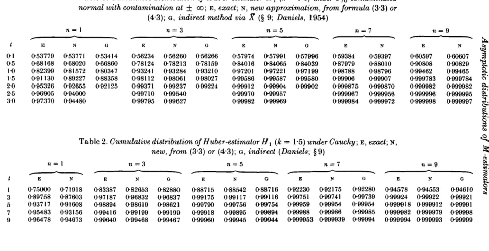
normal ioith contamination at ± oo; E, exact; N, new approximation, from formula (3"3) or

(4-3); G, indirect method via X (§ 9; Daniels, 1954) n = 5 / 0-1 O5 1-0 1-5 2-0 2-5 30 E 0-53779 068168 0-82399 0-91130 0-95326 0-96905 0-97370 N 0-53771 0-68020 0-81572 0-89227 092655 094000 094480 G O53414 066860 O80347 O88358 O92125 E 056234 078124 093241 098112 099371 099710 099795 N O56260 078213 O93284 098061 O99237 O99540 099627 G 056266 O78159 093210 098027 O99224 E O57974 084016 097201 099586 O99912 0-99970 O99982 N 057991 084065 097221 099587 099904 O99957 099969 G 057996 084039 097199 099580 0-99902 E O59384 O87979 O98788 099906 O999875 0999967 O999984 N 059397 088010 098796 099907 0999870 0999956 0999972 E 060597 090808 O99462 0999783 0-999982 0-999996 0999998 N 060607 090829 099465 O999784 0999982 0999995 0999997 n = 1

Table 2. Cumulative distribution of Huber-estimator H1 (Ic = 1-5) under Cauchy; E, exact; N,

new, from (3-3) or (4-3); G, indirect (Daniels; §9)

n = 3 n = 5 n = 7 075000 071918 O89758 087603 003717 091608 E N G G n = 9 G O83387 082653 082880 O97187 096832 O96837 O98894 098619 O98621 088715 088542 088716 092230 092175 092280 O94578 094553 O99175 0-99117 099116 O99751 O99741

099790 099756 099754 O99959 O99954

094610 099739 099924 099922 099921 099954 0999918 0999912 099991 O95483 0-93156 O99416 099199 O99199 O99918 O99895 O99894 O99988 O99986 O99985 O999982 0999979 0-99998 096478 0-94673 O99640 099468 O99467 O99960 O99945 O99944 O999953 0999939 O99994 0-999994 0999993 099999

CO CO

40 CHRISTOPHER A. FIELD AND FRANK R. HAMPEL

|a;| < k,\p{x) = ksgnx if | z | ^ & has been calculated by P. J. Huber by direct convolu-tion and checked in double precision by D. Zwiers for two contaminated normal distributions and by A. Marazzi with fast Fourier transformation via characteristic functions for the Cauchy distribution. The results from our formulae, which were computed by A. Marazzi, using (3-3), and later recomputed by D. Zwiers, using (43), will be compared with these exact distributions.

The e-contaminated normal used by Huber is a standard normal density with probability 1—e plus point masses at ±oo, each with probability ^-e. In our numerical approximations the contaminating point masses were replaced by standard normal distributions at ± 12. For a fine grid of t values, a, and the other constants (cr, at, X3 r, At,) were determined by an iterative search and by integrations using some special properties of the Huber t^-function, in general by numerical integration. Note that these constants remain unchanged as n varies, so they need be computed just once. The approximation (33) for p'n(t)/pn(t) was numerically integrated, exponentiated and again integrated to obtain the normalizing constant and the cumulative distribution. The exact and the approximate values for the 5%-contaminated normal and the Cauchy distribution are given in Tables 1 and 2; more extensive, as well as additional tables can be found in the aforementioned report. Tables 1 and 2 contain also an indirect approximation by means of the saddlepoint method via the arithmetic mean; see §9.

The approximations require significantly less time and storage on the computer than the exact computations. For example, even though the first numerical integration of (3-3), along with several constants, later turned out to be superfluous, since it can be replaced by (4-3), the exact computations for the Cauchy for n = 1 —9 at only 5 points t = 1, 3, 5, 7,9 required more than ten times as much costs and CPU time, 22 min versus 2min on a CDC 6500, than the approximate computations using (33) for a grid of 108 points, t = 0(0-2)7(2)153.

The relative percent error of the tail area 100(N — E)/(1 — E), where N is the approximate and E the exact cumulative, has been calculated. For the contaminated normal with e = 5% the relative error is about or below 1% for t = 0-5 down to n = 1, for t = 1 down to n = 3, for t = 15 down to n = 5. In terms of percentage points, for the same distribution, the relative error is about or below 1% down to n = 3 at the one-sided 5%-point, 7i = s at the 1% 5%-point, n = 7 at the 01%-point and n = 9 at the 001%-point. For the same critical values and sample sizes, the relative errors in the Cauchy case are about or below 7%. It is only with small n and large t that the relative errors become larger and even here the estimate is fairly good; see, for instance, the 5% contaminated normal with n = 3 and t = 30, a relative error of 82%, the actual difference being 0002 (0-99795-0-99627).

Relative tail area errors obtained by use of the first-order approximation p'n(t)/pn(t) — nA2,t, which is the basis for large deviations, § 10, and by use of the third-order formula (41) with renormalization have been computed. They show that a big

Table 3. First and second order terms in (33), written as p'Jpm = nA2+B, along with at,Jor

Hj (k = 1-4) under normal 5%-contaminated at ± oo.

t A2 B a, O2 -0-15803 -0-15129 0-19921 0-4 -0-30867 -0-30939 O39425 0-8 -0-55249 -0-66703 0-75214 1-2 -0-65315 -1-06915 1-02918 1-6 -0-57664 -1-42561 119706 2-0 -0-39724 —1 69161 1-27391

improvement is achieved by inclusion of the second-order term, while the third-order term yields only a small and usually unimportant further improvement. As an example, for the contaminated normal with e = 5°/0,n = 7and< = 1, the relative tail area errors are — 57%, 066% and 025% for the three different orders of approximation. Thus, the second-order formula (3*3), with its nice linearity in n, appears to be the most reasonable one.

The need for including the second-order terms becomes also clear from Table 3, which shows what happens in the KH(t) domain and which also demonstrates nicely the approximate proportionality of the constants with t for small t, corresponding to normality, and the deviations from linearity, even up to downbending of A2,„ for larger t. This complicated behaviour of Kn(t) makes it hard for any expansion about a single point to achieve good accuracy in the tails.

8. RELATIONSHIP TO THE SADDLEPOINT METHOD

The method closest to those used in this paper is the saddlepoint expansion (Daniels, 1954). Hampel (1974a) noted that integration of formula (6-2) for the arithmetic mean gave precisely Daniels's (1954, p. 633) saddlepoint approximation, apart from the normalizing constant. More recently, H. E. Daniels, in a private communication, has shown that (4-2) can also be obtained by means of a saddlepoint approximation. That this is possible is indicated by the close relationship between the saddlepoint approxi-mation and conjugate distributions (Daniels, 1954, p. 639). In fact, the saddlepoint expansion and the expansion starting with (41) {ovpn(t) obviously yield identical results. On the other hand, the expansion ofp'Jpn and the saddlepoint expansion, infinite, and without renormalization, differ in two minor aspects: first, the free constant of integration in logpB to be determined by numerical integration of pn is fixed in the saddlepoint expansion to be log {n* <f>(0)}; secondly, integration and exponentiation of the expansion of p'Jp yields an expansion of pH entirely in the exponent, namely of the form, §10,

pn{t) oc

with a'(t) = ix(t), etc., while in the saddlepoint expansion (2-6) of Daniels (1954) the third and further terms exp{ — y(t)/n—...} are expanded into {l—y(t)/n±...}. This expansion of the exponent can cause finite sections of the saddlepoint expansion to yield negative densities. For the Edgeworth expansion, formulae (10*3), (10*4) and Table 4, an example is given later where expansion of an exponent roughly doubles the approximation error in the best range. However, in our case the first two terms give an excellent approximation, and here the methods differ only by their normalizing constant. The constant of the saddlepoint approximation can be improved (Hampel, 1974a) by using the third, that is l/n, term for t = 0; and as noted by Daniels (1954), it can be even more improved by exact renormalization using numerical or analytical integration. Thus, the second-order formula (3-3) and the saddlepoint approximation with renormalization give identical results.

9. INDIRECT APPROACH VIA ARITHMETIC MEAN

It is possible to utilize the older results for the arithmetic mean in order to derive asymptotic approximations for M-estimators with monotone \p, by noting that the event

T ^ / is essentially the same as the event 11\l/(Xi — t) < 0. Thus one can, for each t separately, determine the approximate cumulative distribution of 7, = £, i/^X, — t)/n by

42 CHRISTOPHER A. FIELD AND FRANK R. HAMPEL

using either the results of Daniels (1954) or Hampel (1974a) for the arithmetic mean of the

if/'s, and then read off pr (Yt ^ 0) = pr(T ^ t). Obviously, this approach needs more

computation than the direct approach; and in the case of M — a-qu&ntiles, the result is not exact even using renormalization, and T, does not even have a density. But, as H. E. Daniels has pointed out, if only a single tail area instead of the full density function is required, this approach is simpler. The accuracy achieved is comparable with that of the direct approach. This is also shown by the numerical results, G in Tables 1 and 2, by Daniels, which are included with his kind permission and which were computed by D. Guest using the saddlepoint approximation for Yt with the renormalization. Both

approximate cumulatives N, direct method, and Q in Tables 1 and 2 are about equally close to E, exact cumulative, but they show different behaviour.

10. RELATIONSHIP TO EDGEWORTH EXPANSION AND LARGE DEVIATIONS

In this section, our formula for p'Jpn and the saddlepoint method are compared to the

classical methods of Edgeworth expansion (Cramer, 1946, pp. 133, 223, 229, etc.; Daniels, 1954, p. 635) and large deviations (Richter, 1957, pp. 212, 214; Feller, 1966, p. 520, etc.; Cramer, 1938). In addition, from the formula for p'Jpm some other variants,

including a new variant of the Edgeworth expansion, are derived.

First we recall that our expansions for p'H(t)/pH(t) and pn(t) as well as the saddlepoint

method differ from other methods by expanding not only at one point t = 0, but rather at every t. For the arithmetic mean, this is merely a shift in ifn-space:

h't(x)/ht(x) =f'(x)/f(x) + at. All three methods utilize the Edgeworth expansion only at

the expectation, though in slightly different ways; see also Daniels (1954, p. 634) for relations between saddlepoint approximation and Edgeworth expansion.

To facilitate comparisons we consider the arithmetic mean TH = Xn with density pn of

independent identically distributed observations Xt with underlying density / and

E{X,) = 0, var (X,) = a2, E(X?)/o3 = X3, E{Xf)/a*-3 = kA.

Assume / fulfills all necessary regularity conditions such as those of Richter (1957, p. 208).

Assume that the following general form of expansion basic to this paper holds:

P'At)/Pn(t) = -n<x(t)-p(t)-y(t)/n-..., (10-1)

where a(t) = a, and fi(t) = X3 J(2ot) in the previous notation. Now expand the terms into

Taylor series around t = 0: a(t) = a(0) + a'(0)t+±a"(0)t2 +..., etc. Integration yields

-y(0)t/n-$y'(0)t2/n-.... (10-2)

We assume that the constant of integration can be expanded as QB = log {n/(2no2)}*(l +<ojn+...).

Exponentiation of (102) yields a doubly infinite expansion for pn(t), from which most

other known expansions can be derived, as well as new ones.

The main question is at which rate t —* 0 as n —> oo. If we aim for good accuracy at a fixed multiple of the standard deviation of the distribution of Tn, as does the Edgeworth

expansion, we are led to the choice nt2 = const > 0. This choice induces an ordering of

The leading terms up to third order using A4, which empirically seem to give a good fit near 0 even for small n, are, using a(0) = 0 because of centring,

pn(t) ^ {n/(27ta2)}±exp{-i7ia'(0)<2}

x exp { - a"(0) nt3/6 - 0(0) t - a(3)(0) n/4/24 - \fi\0) t2 + OJ Jn). (103) Expansion of the second exponential yields precisely the usual third-order Edgeworth approximation and corresponding expansion of the infinite series obviously yields the Edgeworth series:

pn(t) — {n/(27t<72)}*exp{— %na'(0)t2}

x {1 -a"(0) ni3/Q-p(0) *-a<3)(0) nt*/24-tf'(0) t 0)2 n2 «6/72 (1O4) Comparison of terms, e.g. with Cramer (1946, p. 229), provides the bridge to the moments of the Xt:

a(0) = 0, a"(0)= -/l3/(73, = kJ(2o2)-k2/G2,

a(3)(0) =

(10-5) Formula (1O3), which we may call 'Edgeworth in exponent', proves in an example, Table 4, to be about twice as good as Edgeworth (104) in the central region where both are good. Outside about two standard deviations of Tn from its mean both are very bad; so it matters little that (103) loses the norming of (104) and may sometimes explode, namely if A4 —3A3 ^ 0 and not X3 = A4 = 0, while (104) may lead to negative densities.

There are, of course, many possibilities for the speed with which / —» 0. For instance, the expansion with nt = const has as its leading term

pn(t) ^ {n/(27tff2)}*exp{-i7M£'(0)f2-^(0)< + cu1/n}.

This is the nonnormalized 'best fitting normal density' which uses A3 for a shift of the mean and in addition A4 for approximate adjustment of the height at t = 0. The normalized counterpart can be obtained from the expansion of (10-1) around t = 0 by integrating p'n(t)/pH(t) — — na'(0)t — fi(0). These and other variants were studied for the

Table 4. Comparison of approximations for density of mean of four independent exponen-tially distributed observations

Large Exact EDG exp EDO Norm. dev.

I 025 0 0-25 0-5 0-75 ] 1-25 1-5 1 75 2 density 0 0 0-24525 0-72179 089617 078147 056150 O35694 020852 011451 (1O3) 000168 004596 029544 070413 089126 O78143 056358 036151 020305 008952 %err. 205 -2-4 -O5 - O 0 0 5 O4 1-3 -2-6 -21-8 (10-4) - 0 0 3 9 2 0 002175 029765 O69231 O88857 078126 O56584 O36968 020052 009373 % err. 21-4 -41 -O8 - O 0 2 08 3-6 -3-8 - 1 8 1 approx. O0350 O1080 O2590 O4840 O7042 07979 O7042 O4840 02590 O1080 % err. 5-6 — 11-9 -21-4 21 25-4 35-6 24-2 -5-7 (10-6) 00002 O0105 O1076 O3848 06869 07979 07162 05371 03313 O1507 % err. -56-1 -46-7 -23-4 21 27-6 50-5 58-9 31-6 Approximation (3-3) is exact in this case (Daniels, 1954, p. 636), and the saddlepoint approximation without renormalization has constant relative error of +2-1%.

EDO exp, Edgeworth in exponent; norm, approx., normal approximation; large dev., large deviations; % err., % error.

44 CHRISTOPHER A. FIELD AND FRANK R. HAMPEL 9 — 8 -7 — 6 — 5 — 4 — 3 — 2 — 1 — 0 - 0 - 9 0 9 9 - 0 - 9 9 9 5 - 0 - 9 9 9 - 0-9975 - 0 - 9 9 5 - 0 - 9 9 - 0 - 9 7 5 - 0-95 - 0 - 9 - 0 - 8 * - 0-7 ^ T -(Hi, : / : / : / / • / / / . ' / / / • / / / • / / / / / /

-A '

/ '

/

sf ^—^^-^ Exact 4 small-sample asymptotic ^F Edgeworth

Jr ~~ ~~ ~~ — Large deviations ^ ^ —•—•—• Normal approximations

1 1 1 1

0-1 0-2 0-3 0-4 0-5

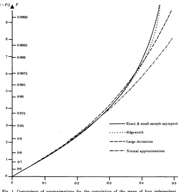
Fig. 1. Comparison of approximations for the cumulative of the mean of four independent uniformly distributed data, in logistic scale. Compared with the exact cumulative of XA under

£/(—i.i) are Edgeworth (10-4), large deviations (10-6) and normal approximation; the new approximation (3-3) or (4-3) coincides with the exact cumulative within drawing accuracy.

example of Table 4, but are not pursued here because of lack of space. Some conclusions are that the precise aims of mediocre simple fits have to be selected first and that renormalization may be much less suitable here than for the globally good approxi-mations related to the saddlepoint technique.

An extreme case of asymptotic 'directions' in (102) is first to let n -» oo and then t —> 0 or the limiting case of nc t = const for c -+ 0. This amounts to keeping only the leading constant term and the expansion of a(t) and leads precisely to the large deviations expansion for pa(t). The usual large deviations approximation using A4 becomes (Richter, 1957)

pn(t) ^ (106)

Now it is known from a number of examples that for small n the ft terms are definitely needed to give a good approximation. Hence it can be expected that even the full infinite large deviations expansion will give a bad fit except for very large n, but it is still remarkable that in the two examples computed in this paper, Table 4 and Fig. 1, formula (106) is even worse than the normal approximation. The large deviation formulae for the cumulative distribution ofTn, as given, for example, by Feller (1966, p. 520), contain an additional approximation, namely of the normal tail area, and hence are not likely to fit any better.

If we go to the other extreme in the choice of asymptotic 'directions' and let first t —• 0 and then n -* oo, we obtain the expansion of QB, albeit only for logj)n(0). This is almost the same as the saddlepoint series expansion (2-6) of Daniels (1954) for t = 0, there x = 0, the latter differing again in having the exponential expanded into a sum. However, the expansion of ft, is still unknown beyond the first two terms.

For completeness, we note the obvious facts that the first terms of (103), (104) and (106), up to using a'(0), are merely the normal approximation; that the latter, (10-6) and the saddlepoint approximation, the leading term of the saddlepoint expansion, coincide for t = 0; and that from (10-1) a'(O) = 1/«T2 is the limit of the derivative of p'H{t)lpH{t) divided by n at t = 0, namely of the inverse standardized local variance at t = 0.

The authors are very grateful to H. E. Daniels, the first worker in the field, for very pleasant cooperation, many stimulating discussions and for contributing the com-putations with the indirect method; to P. J. Huber for his permanent interest, support of the second author and for supplying his exact computations for Z/^l-4); to the Forschungsinstitut fur Mathematik, ETH Zurich for their support of the first author; to A. Marazzi, D. Guest and D. Zwiers for careful computer computations; and to a referee for very thorough and detailed comments which led to considerable changes and improvements of the earlier research report.

REFERENCES

BABNDORFF-NIELSEN, O. & Cox, D. R. (1979). Edgeworth and saddle-point approximations with statistical applications (with discussion). J. R. Statist. Soc. B 41, 279-312.

CRAMER, H. (1938). Sur un nouveau theoreme-limite de la theorie des probability. Act-ualites Scientifiques et

industrieUes 736. Paris: Hermann <fe Cie.

CRAMER, H. (1946). Mathematical Methods of Statistics. Princeton University Press.

DANIELS, H. E. (1954). Saddlepoint approximations in statistics. Ann. Math. Statist. 25, 631-50. DANIELS, H. E. (1980). Exact saddlepoint approximations. Biometrilca 67, 59-63.

DUBBIN, J. (1980a). Approximations for densities of sufficient estimators. Biometrilca 67, 311-33. DURBIN, J. (1980b). The approximate distribution of partial serial correlation coefficients calculated from

residuals from regression on Fourier series. Biometrika 67, 335-49.

FELLER, W. (1966). An Introduction to Probability Theory and its Applications, Vol. II. New York: Wiley. FIELD, C. A. (1978). Summary of small sample asymptotics. In Proceedings of the Second Prague Symposium

on Asymptotic Statistics, Ed. P. Mandl and M. Huskova, pp. 173-80. Prague: Society of Czechoslovak

Mathematicians and Physicists, Charles University.

HAMPEL, F. R. (1971). A general qualitative definition of robustness. Ann. Math. Statist. 42, 1887-96. HAMPEL, F. R. (1974a). Some small sample asymptotics. In Proceedings of Prague Symposium on Asymptotic

Statistics, 1973, Vol. II, Ed. J. Hajek, pp. 109-26. Prague: Charles University.

HAMPEL, F. R. (1974b). The influence curve and its role in robust estimation. J. Am. Statist. Assoc. 69, 383-93.

HUBER, P. J. (1964). Robust estimation of a location parameter. Ann. Math. Statist. 35, 73-101.

HUBER, P. J. (1977). Robust Statistical Procedures. CBMS-NSF Regional Conference Series in Applied Mathematics Xo. 27. Philadelphia: Society for Industrial and Applied Mathematics.

46 CHRISTOPHER A. FIELD AND FRANK R. HAMPEL

KHTNCHIN, A. I. (1949). Mathematical Foundations of Statistical Mechanics. New York: Dover.

RICHTEB, W. (1957). Local limit theorems for large deviations. Theory Prob. Applic. 2, 206-20. [Received September 1978. Revised June 1981]