©International Epidemiological Association 1990 Printed in Great Britain
The Use of Measures of Influence in
Epidemiology
ULRICH HELFENSTEIN* AND CHRISTOPH MINDER*
Helfenstein U (Biostatistical Centre for the Medical Department, University of Zurich, Plattenstrasse 54, CH-8032, Zurich, Switzerland) and Minder C. Internationa/Journal of Epidemiology 1990,19: 197-204.
In epidemiological studies the units of observation often consist of political entities such as countries, each of which has its own specific inner structure. When a multiple regression is performed it is therefore of particular interest to ana-lyse not only the overall behaviour of the dataset, but in addition, to investigate how each individual country contrib-utes to, and deviates from, this overall behaviour.
By means of the example 'relation between infant mortality and structural data of countries' several ways are dis-cussed of how each individual country can influence the regression model. Firstly the potential influence which each country might exhibit due to the explanatory variables alone is analysed. Then the actual influence of each country is analysed by taking the explanatory variables and the target variable into account simultaneously. This is done by means of statistical measures not generally familiar to epidemiologists, which have been developed in recent years (leverage values, Cook's distances). These measures also point to deviations of countries from the model, and suggest directions in which to search for explanation. Finally the influence of the 'size' of the countries is investigated.
When a multiple regression is performed to analyse data, results and interpretations are usually based on summary statistics such as slopes, coefficient of deter-mination and others.1 In epidemiological studies,
how-ever, the units of observation often consist of countries or other political entities, each of which has its own specific inner structure. When a multiple regression is performed it is therefore of particular interest to ana-lyse not only the overall behaviour of the dataset, but in addition, to investigate how each individual country contributes to, and deviates from, this overall behav-iour. Similar deliberations apply to ecological or sur-veillance studies where the units of observation consist of groups of people such as occupations, social classes, communities, etc. Subsequently, an example is pre-sented to illustrate some of the concepts underlying measures of influence: The relation between infant mortality and structural data of countries.
Several ways are described how each individual country may influence the regression model and there-fore the conclusions about the relation between infant mortality and structural data. Firstly, we consider the potential influence of each country due to its values of the explanatory structural variables alone. Then the
'Biostatistical Center of the Medical Department, University of Zurich Plattenstrasse 54, CH-8032 Zurich, Switzerland.
"Institut fur Sozial- und Praventivmediiin, Finkenhubelweg 11, CH-3012 Bern, Switzerland.
actual influence of each country is analysed by taking its values for explanatory variables and target variable simultaneously into account. This is done by means of case statistics, statistical measures which have been developed during the last years.23 They are presented
in the next section. These analyses will also point-to deviations of countries from the model, and suggest directions in which to search for explanation.
A further particularity of this kind of data is that the units of observation may differ strongly in 'size'. Approximately one-fifth of the world population lives in China. It seems therefore at first sight evident that China should receive a much larger weight than a 'small' country. This conclusion is, as will be shown, however, doubtful.
Subsequently the relation between infant mortality and structural data of 125 countries with more than one million inhabitants each is investigated. The data stem from the UN, the world bank and the OECD. A larger set of structural data may be found in the 'Weltalma-nach' 1986.4 In our example, infant mortality is the
tar-get variable and the explanatory variables are: number of inhabitants, density of population, gross domestic product per capita ($), food supply in per cent, imported area cultivated (%), number of inhabitants per physician and illiteracy (%). These data describe different characteristics of a country, like economic situation, educational standard of the population, medical supply etc. The regression is used to investi-197
gate which combination of these structural variables can best 'explain' infant mortality. For ease of refer-ence the data4 are presented in Table 1.
Several investigations about relations between infant mortality and explanatory variables have been published, all using overall statistics which arise from regression models. Since the main concern of the pres-ent study is the use of influence measures, we refer to the article of Woodhandler and Himmelstein5 for a
review of past work on these relationships. STATISTICAL METHODS
Firstly, the different sources of the influence which the individual countries exert on the regression model are explained then the precise mathematical formulae are given, with graphs of the particular example given to assist interpretation.
Potential Influence
One aspect of influence is determined by the values of the explanatory variables. The case statistics describ-ing this aspect are called leverage values.6 The closer
the values of the regressor variables lie to the border of the observed region, the larger are the corresponding leverage values (compare Figure 3 and its description in the next sections). Since the values of the target vari-able do not enter into these statistics, it is possible that a case with a large leverage value turns out to have no marked influence on the model. To emphasize this aspect, Cook and Weisberg7 call them potential values.
In order to give a mathematical formula to this con-cept, assume that the relation between the target vari-able and the p explanatory varivari-ables is represented by the regression model:
( l ) y = Xp + e
y is the vector of observed responses, X is the matrix of explanatory data and e is a random vector with mean O and covariance matrix a2l. The vector of fitted
responses y may be obtained from y by the linear operation:
(2)y = Hy,
where H = X(XTX)'XT is called the 'hat' matrix
because it transforms the vector y into the vector of fit-ted responses y. The diagonal elements hu of the hat
matrix H are called potential values (or leverage values).6
A helpful representation of h^ is given by: (3) h;i = 1/n + (Jessys,"1 (x-x) I (n-1),
where S, is the covariance matrix of the explanatory variables. This case statistic has a useful geometric interpretation: If the term 1/n on the right side is dropped, remainder is proportional to the Mahalano-bis distance from x-t to the centre x. Points lying on
elliptical contours have the same Mahalanobis distance from the centre and therefore the same potential influ-ence on the regression model.
Actual Influence
Cook's distance. A further aspect of influence is deter-mined by the residuals ie by the deviations of the observed values of the target variable (infant mor-tality) from the fitted values. Potential values and resi-duals are combined into a single case statistic called Cook's distance.6 This measure contains information
from the explanatory variables and from the target variable and it determines the actual influence of each country on the model.
In mathematical terms Cook's distance of the i-th country is given by6:
(4) D, = (1/p) r,2 ( M l - h a ) ) .
where r, = e ^1 (l-h^)"2
D; is essentially composed of two parts: The first is the square of the studentized residual r,, ie a measure of the discrepancy between the observed and the fitted value corrected for its individual precision. The second part is a monotonic increasing function of the i-th potential value hH. Thus, a large value of D, may be due
to large ri( large hu, or both.
Size of the units. Different approaches have been sug-gested to solve the problem of'size' (different number of inhabitants, infants, etc). In their investigation of cardiovascular mortality rates in 161 local authorities in England, Fryer et a/.8 eg proposed the use of weights
inversely proportional to binomial variance. Pocock et aP performed a thorough statistical analysis of the problem. They found that the variation of mortality rates between political units is composed of three components:
(i) explained variation; (ii) unexplained variation; (iii) binomial sampling variation.
The explained variation (i) is of interest because it can contribute to a better understanding of a disease process and its possible causes. Since one can not expect to include all explanatory variables, the com-ponent (ii) is present. In each country the number of infants may be thought of as being a sample of a hypo-thetical population with an unknown 'true' mortality rate. This leads to component (iii); (ii) and (iii) together give the variation about regression.
The 'size' of the countries or the number of infants are only of concern with regard to the binomial varia-tion (iii). If the binomial variavaria-tions are small, the unex-plained component (ii) dominates, and a weighted regression may lead to an overweighting of the 'large' countries and thus distort the results. If the
unex-199
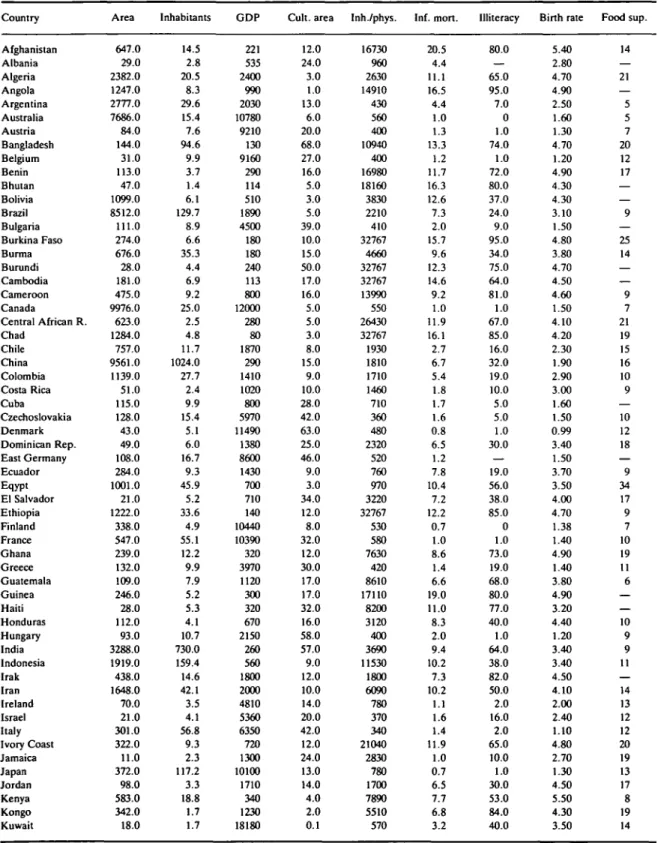
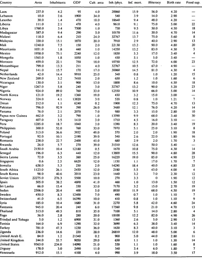
TABLE 1 The data: Structural data of countries. Country Afghanistan Albania Algeria Angola Argentina Australia Austria Bangladesh Belgium Benin Bhutan Bolivia Brazil Bulgaria Burkina Faso Burma Burundi Cambodia Cameroon Canada Central African R. Chad Chile China Colombia Costa Rica Cuba Czechoslovakia Denmark Dominican Rep. East Germany Ecuador Eqypt El Salvador Ethiopia Finland France Ghana Greece Guatemala Guinea Haiti Honduras Hungary India Indonesia Irak Iran Ireland Israel Italy Ivory Coast Jamaica Japan Jordan Kenya Kongo Kuwait Area 647.0 29.0 2382.0 1247.0 2777.0 7686.0 84.0 144.0 31.0 113.0 47.0 1099.0 8512.0 111.0 274.0 676.0 28.0 181.0 475.0 9976.0 623.0 1284.0 757.0 9561.0 1139.0 51.0 115.0 128.0 43.0 49.0 108.0 284.0 1001.0 21.0 1222.0 338.0 547.0 239.0 132.0 109.0 246.0 28.0 112.0 93.0 3288.0 1919.0 438.0 1648.0 70.0 21.0 301.0 322.0 11.0 372.0 98.0 583.0 342.0 18.0 Inhabitants 14.5 2.8 20.5 8.3 29.6 15.4 7.6 94.6 9.9 3.7 1.4 6.1 129.7 8.9 6.6 35.3 4.4 6.9 9.2 25.0 2.5 4.8 11.7 1024.0 27.7 2.4 9.9 15.4 5.1 6.0 16.7 9.3 45.9 5.2 33.6 4.9 55.1 12.2 9.9 7.9 5.2 5.3 4.1 10.7 730.0 159.4 14.6 42.1 3.5 4.1 56.8 9.3 2.3 117.2 3.3 18.8 1.7 1.7 GDP 221 535 2400 990 2030 10780 9210 130 9160 290 114 510 1890 4500 180 180 240 113 800 12000 280 80 1870 290 1410 1020 800 5970 11490 1380 8600 1430 700 710 140 10440 10390 320 3970 1120 300 320 670 2150 260 560 1800 2000 4810 5360 6350 720 1300 10100 1710 340 1230 18180 Cult, area 12.0 24.0 3.0 1.0 13.0 6.0 20.0 68.0 27.0 16.0 5.0 3.0 5.0 39.0 10.0 15.0 50.0 17.0 16.0 5.0 5.0 3.0 8.0 15.0 9.0 10.0 28.0 42.0 63.0 25.0 46.0 9.0 3.0 34.0 12.0 8.0 32.0 12.0 30.0 17.0 17.0 32.0 16.0 58.0 57.0 9.0 12.0 10.0 14.0 20.0 42.0 12.0 24.0 13.0 14.0 4.0 2.0 0.1 Inh./phys. 16730 960 2630 14910 430 560 400 10940 400 16980 18160 3830 2210 410 32767 4660 32767 32767 13990 550 26430 32767 1930 1810 1710 1460 710 360 480 2320 520 760 970 3220 32767 530 580 7630 420 8610 17110 8200 3120 400 3690 11530 1800 6090 780 370 340 21040 2830 780 1700 7890 5510 570 Inf. mort. 20.5 4.4 11.1 16.5 4.4 1.0 1.3 13.3 1.2 11.7 16.3 12.6 7.3 2.0 15.7 9.6 12.3 14.6 9.2 1.0 11.9 16.1 2.7 6.7 5.4 1.8 1.7 1.6 0.8 6.5 1.2 7.8 10.4 7.2 12.2 0.7 1.0 8.6 1.4 6.6 19.0 11.0 8.3 2.0 9.4 10.2 7.3 10.2 1.1 1.6 1.4 11.9 1.0 0.7 6.5 7.7 6.8 3.2 Illiteracy 80.0 65.0 95.0 7.0 0 1.0 74.0 1.0 72.0 80.0 37.0 24.0 9.0 95.0 34.0 75.0 64.0 81.0 1.0 67.0 85.0 16.0 32.0 19.0 10.0 5.0 5.0 1.0 30.0 — 19.0 56.0 38.0 85.0 0 1.0 73.0 19.0 68.0 80.0 77.0 40.0 1.0 64.0 38.0 82.0 50.0 2.0 16.0 2.0 65.0 10.0 1.0 30.0 53.0 84.0 40.0 Birth rate 5.40 2.80 4.70 4.90 2.50 1.60 1.30 4.70 1.20 4.90 4.30 4.30 3.10 1.50 4.80 3.80 4.70 4.50 4.60 1.50 4.10 4.20 2.30 1.90 2.90 3.00 1.60 1.50 0.99 3.40 1.50 3.70 3.50 4.00 4.70 1.38 1.40 4.90 1.40 3.80 4.90 3.20 4.40 1.20 3.40 3.40 4.50 4.10 2.00 2.40 1.10 4.80 2.70 1.30 4.50 5.50 4.30 3.50 Food sup. 14 — 21 — 5 5 7 20 12 17 — 9 — 25 14 — — 9 7 21 19 15 16 10 9 — 10 12 18 — 9 34 17 9 7 10 19 11 6 — 10 9 9 11 — 14 13 12 12 20 19 13 17 8 19 14
TABLE 1 Continued Country Laos Lebanon Lesotho Liberia Libya Madagascar Malawi Malaysia Mali Mauritania Mexico Mongolia Morocco Mozambique Nepal Netherlands New Zealand Nicaragua Niger Nigeria North Korea Norway Oman Pakistan Panama
Papua new Guinea Paraguay Peru Philippines Poland Portugal Romania Rwanda Saudi Arabia Senegal Sierra Leone Singapore Somalia South Africa South Korea Soviet Union Spain Sri Lanka Sudan Sweden Switzerland Syria Tanzania Thailand Togo
Trindad and Tobago Tunisia Turkey Uganda United Arab E. United Kingdom United States Urguay Venezuela Area 237.0 10.0 30.0 111.0 1760.0 587.0 118.0 330.0 1240.0 1031.0 1958.0 1565.0 459.0 799.0 141.0 42.0 269.0 130.0 1267.0 924.0 121.0 324.0 212.0 796.0 76.0 462.0 407.0 1285.0 300.0 313.0 92.0 238.0 26.0 2150.0 196.0 72.0 0.6 638.0 1123.0 98.0 22275.0 505.0 66.0 2506.0 450.0 41.0 185.0 945.0 513.0 56.0 5.0 164.0 781.0 236.0 84.0 244.0 9363.0 178.0 912.0 Inhabitants 4.2 2.6 1.4 2.1 3.4 9.4 6.4 15.1 7.5 1.8 75.1 1.8 22.1 13.3 15.7 14.4 3.2 3.1 5.8 89.0 19.2 4.1 1.1 92.9 2.1 3.2 3.5 18.7 52.0 36.6 10.1 22.7 5.7 10.4 6.3 3.5 2.5 5.3 26.1 40.6 276.3 38.2 15.4 20.4 8.3 6.5 10.4 20.4 49.5 2.8 1.2 6.9 47.3 14.6 1.2 55.7 234.0 3.0 15.1 GDP 95 1900 470 470 7500 290 210 1870 150 440 2240 1050 750 211 170 9910 7410 900 240 760 1360 13820 6240 390 2070 790 1410 1040 760 3952 2190 2400 270 12180 440 380 6620 250 2450 2010 5500 4800 330 400 12400 16390 1680 240 810 280 6900 1290 1230 220 21340 9050 14090 2490 4100 Cult, area 4.0 34.0 10.0 4.0 1.0 5.0 24.0 20.0 2.0 1.0 12.0 1.0 18.0 4.0 17.0 25.0 2.0 13.0 3.0 33.0 19.0 3.0 0.2 26.0 7.0 1.0 3.0 3.0 33.0 49.0 39.0 45.0 39.0 0.5 12.0 25.0 12.0 2.0 12.0 23.0 10.0 41.0 33.0 5.0 7.0 10.0 31.0 6.0 35.0 20.0 31.0 32.0 36.0 28.0 0.2 29.0 21.0 11.0 4.0 Inh./phys. 20060 540 18640 9610 730 10170 32767 7910 22130 14350 1830 450 10750 32767 30060 540 650 1800 32767 12550 430 520 1900 3480 980 13590 1710 1390 7970 570 540 680 31510 1670 13800 16220 1150 14290 2180 1440 270 460 7170 8930 490 410 2270 17560 7100 18100 1360 3690 1630 26810 900 650 520 540 990 Inf. mort. 15.9 3.9 9.4 9.1 9.5 11.6 13.7 2.9 13.2 13.2 5.3 5.1 12.5 10.5 14.5 0.8 1.2 8.6 13.2 10.9 3.2 0.8 12.3 12.1 3.3 9.9 4.5 8.3 5.1 2.0 2.6 2.9 12.6 10.8 15.5 19.0 1.1 18.4 5.5 3.2 3.3 1.0 3.2 11.9 0.7 0.8 5.8 9.8 5.1 12.2 2.6 6.5 8.3 12.0 5.0 1.1 1.1 3.4 3.9 Illiteracy 56.0 14.0 48.0 75.0 50.0 50.0 75.0 40.0 90.0 83.0 17.0 5.0 72.0 67.0 • 81.0 1.0 1.0 10.0 90.0 66.0 15.0 1.0 75.0 76.0 15.0 68.0 16.0 20.0 25.0 2.0 22.0 2.0 50.0 75.0 90.0 85.0 17.0 40.0 43.0 7.0 0 13.0 15.0 68.0 1.0 1.0 42.0 21.0 14.0 82.0 5.0 38.0 40.0 48.0 44.0 1.0 1.0 6.0 18.0 Birth rate 4.20 2.90 4.20 5.00 4.50 4.70 5.60 2.90 4.80 4.30 3.40 3.40 4.00 4.90 4.30 1.20 1.60 4.50 5.20 5.00 3.00 1.21 4.70 4.20 2.80 3.40 3.10 3.40 3.10 1.90 1.80 1.70 5.40 4.30 4.80 4.90 1.70 4.80 4.00 2.30 1.90 1.50 2.70 4.50 1.10 1.10 4.60 4.70 2.80 4.90 2.90 3.40 3.10 5.00 2.80 1.30 1.60 1.80 3.50 Food sup. — — 22 18 14 8 13 20 5 4 — 23 — 4 15 6 18 23 14 — 7 13 14 10 30 — 19 8 18 16 3 — 14 28 23 7 33 4 12 12 12 19 19 7 9 24 13 4 26 13 14 3 6 11 14 8 7 17
MEASURES OF INFLUENCE IN EPIDEMIOLOGY TABLE I Continued Country Vietnam West Germany Yemen (Aden) Yemen (Sana) Yugoslavia Zaire Zambia Zimbabwe Area 333.0 249.0 333.0 195.0 256.0 2345.0 753.0 391.0 Inhabitants 57.2 61.0 2.1 6.2 22.9 31.2 6.2 7.7 GDP 180 11420 510 510 2570 160 580 740 Cult, area 18.0 31.0 0.6 14.0 31.0 3.0 7.0 8.0 Inh./phys. 4190 450 7200 11670 550 14780 7670 6580 Inf. mort. 5.3 1.2 14.0 16.3 3.4 10.6 10.5 8.3 Illiteracy 13.0 1.0 60.0 79.0 15.0 45.0 56.0 21.0 Birth rate 3.50 1.00 4.80 4.80 1.50 4.60 5.00 5.40 Food sup. _ 12 — 28 6 — — — Abbreviations are explained in the text. A dash indicates a missing value.
plained variation (ii) disappears, weighted regression with weights inversely proportional to the binomial variance needs to be applied.
In order to give a precise formula to the above con-cepts, denote the number of infants in the country with index i (i=l, . . ., 125) by n.j. During a certain time interval d, of the infants died. The observed mortality rate is y> = d/n,. The 'true' unknown death rate is nr
For the observed rate yt we may then write: (5) y, = *, + | ,
li has a shifted binomial distribution with expectation 0 and variance Xj2 = JI,(1—JT.;)/^ (when n, is large |( is
approximately normally distributed). Now, the n-, are related to the explanatory variables by the usual multiple linear regression:
(6)jii = p0 + p1xl i+ . . . . + ppixpi + e,.
The e, describe the unexplained part of the nr They have the constant variance o2. The p regressor
vari-ables describe the explained part. Combining (1) and (2) we get:
(7)yi = P0 + P , xI I+ . . . . +Ppixpi + Tii,
rig is a random variable with expectation 0 and variance (8) a2 + xi(l-n)/ni.
As one can see, the number of infants n; only affects
the tj2 = Jtj(l—jr.,) In,. If the T,2 are small compared to
the unexplained component a2, the latter dominates
the regression error. In this situation, binomial weight-ing may lead to an overweightweight-ing of the 'large' countries. If on the other hand o2 = 0, the correct
solu-tion is given by the regression with weights propor-tional to Tj'2.
Pocock et at have proposed a maximum likelihood method, designed to estimate error components and parameters.
RESULTS
In order to explain infant mortality rates, the following structural variables were used (see Table 1): Number of inhabitants, density of population (inhabitants per area), gross domestic product per capita ($), food
sup-plies in per cent of imports, area cultivated (%), number of inhabitants per physician and illiteracy (% of population). Some of these variables, eg the gross domestic product, have a skewed distribution and hence were transformed logarithmically ('symmetrization').
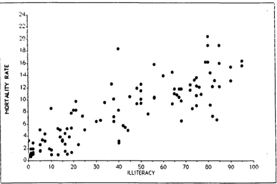
First a stepwise multiple regression was performed without weighting the countries. From all available explanatory variables the regression showed up only two as significant: illiteracy (ILL-IT) and gross dom-estic product per capita (GDP). The relation between each of these variables and infant mortality is pre-sented in Figures 1 and 2.
In a second step the procedure proposed by Pocock et at was applied to estimate the binomial component of the variance about regression (compare last sec-tion). This binomial part was found to be only 0.64%o. The variation about regression is therefore dominated by the unexplained component: a regression with Pocock's method gives practically the same results as the unweighted regression.
With the two explanatory variables ILLIT and GDP, both methods gave the same coefficient of determina-tion R2 = 0.82. Additional explanatory variables did
not increase R2 significantly.
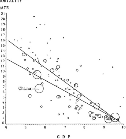
The regression with binomial weights leads to a dif-ferent result. The effect of weighting is illustrated in Figure 2. The figure shows a marked negative correla-tion between infant mortality and GDP. In this picture the individual countries are not represented by points as usual, but rather by circles. The areas of the circles are proportional to the binomial weights of the corre-sponding countries. The two straight lines are calcu-lated from simple regressions with and without weighting. The straight line of the weighted regression is markedly displaced downwards due to the large influence of China.
In order to find out which countries exert the strongest potential and actual influence on the regres-sion model, leverage values and Cook's distances were
24, 20 13 16 14 12 10 8 6 4-2i 0* • » \ 10 20 30 40 50 60 ILLITERACY 70 eo 90 100
FIGURE 1. Relation between mortality rates and illiteracy. calculated for each country (see earlier). Figure 3
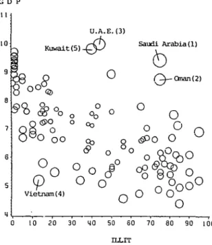
shows the position of each country in the space of the two explanatory variables ILLIT and GDP ('X-space'). In this figure, areas of circles are proportional to leverage values. The countries with the largest lever-age values are Saudi Arabia, Oman, United Arab Emirates (UAE), Vietnam and Kuwait. These countries have the strongest potential influence on the regression. As the figure shows the position of these countries is on the border of the 'X-space'.
Analogous to Figure 3, Figure 4 shows the actual influence as measured by Cook's distance as areas of circles in 'X-space'. The countries with the largest Cook's distances are Somalia, Congo, Afghanistan, Iraq, Oman and Saudi Arabia. These countries have the strongest actual influence.
DISCUSSION
In the following discussion the problems due to the dif-ferent 'sizes' of the countries are considered first. Sub-sequently the 'overall' results are described, and the potential and actual influences of the individual countries are discussed. Finally the stability of the identified regression model is investigated under inclusion and exclusion of the countries with the largest actual influence.
The differences in 'size' ie in number of births between the countries are very large. China eg has
almost 600 times as many births per year than the UAE. This gave rise to the question of appropriately weighting the countries. The application of Pocock's9
method to the present data showed that the proportion of residual variance due to sampling is almost zero and that therefore all countries should receive the same weight. This finding contradicts the intuitive impres-sion which suggests that China should receive a much larger weight than eg Bhutan. China and Bhutan pro-vide the same amount of information about the relation between infant mortality and explanatory variables. Their influence on the regression model due to size should therefore be the same.
Performing the appropriate unweighted ^stepwise regression the following 'overall' results were found: Out of all available explanatory variables the regres-sion selected only two: illiteracy and GDP per capita. The variable illiteracy alone gave a coefficient of deter-mination R2 = 0.75, ie 75% of the variation in infant
mortality is 'explained' by illiteracy (Figure 2). The second variable able to enlarge markedly R2 was GDP
(R2 = 0.82, partial F-test: P<0.0001).
No additional regressor variable (eg number of inhabitants per physician) did increase R2 significantly.
It is therefore found that illiteracy plays a major role in 'explaining' infant mortality. In particular, it explains more of the variation than GDP. These results are con-sistent with the findings of Sagan and Afifi.10 In their
MEASURES OF INFLUENCE IN EPIDEMIOLOGY MORTALITY RATE 21 20 19 18 17 16 15 13 12 11 10 9 8 7 6 5 3 2 1 0 H 5 6 7 8 9 10 G D P
FIGURE 2. Relation between mortality rates and GDP per capita (logarithmically transformed). Size of the areas proportional to the weights. Upper
straight line: without weighting. Lower straight line: with weighting.
investigation about the relation between infant mor-tality, energy consumption and other variables they found that illiteracy had the largest coefficient of corre-lation with infant mortality.
Figure 3 shows the potential influence which each country exerts on the model due to the values of the explanatory variables alone, ie to its position in 'X-space'. The areas of the circles are proportional to the potential values of the corresponding countries. One recognizes clearly that the closer a country lies towards the border of the 'X-space', the stronger is its potential influence.
The following countries have the largest 'distance' from the centre in X-space and therefore the largest potential influence: Saudi Arabia, Oman, UAE, Viet-nam and Kuwait; four of these are oil-rich countries. As one can see from the figure, they have a common characteristic property: A high degree of illiteracy inspite of the relatively high GDP. Vietnam has the fourth largest potential influence. Its position in 'X-space' is just opposite to the oil-rich countries: Even
though the GDP is relatively low, illiteracy is relatively low.
Analogous to Figure 3, Figure 4 shows the actual influence of each country. Here the areas of the circles are proportional to Cook's distances. This case statistic combines information from the leverage values and from the residuals. It measures the actual influence of each unit on the regression. Comparing the potential influence of the four oil-rich countries (Figure 3) with their actual influence (Figure 4), one sees that these countries split in two groups. While the actual influ-ence of Saudi Arabia and Oman is strong, the influinflu-ence of UAE and Kuwait is weak. UAE and Kuwait cer-tainly have large potential values but their residuals are small. This means that even though they are far from the centre in X-space, their observed infant mortality corresponds to what one expects on the basis of the regression model. In contrast to this, Saudi Arabia and Oman also have large Cook's distances. Infant mor-tality in these countries is larger than one would expect from the model (positive residuals).
G D P 11 10 9 8 7 6 5 M
I
Kuwait(5) §•%8^
(
j (5>O o'o oo
O o
Vietnam(4) U.A O °o>°c
-E.(3) )0
o oo °o
)
o
Saudi Arabia(l)o
o
o
°
Oo
(^-Qran(2)O
° o
o o ^
^ ) O
O
o OO
o
0 10 20 30 40 50 60 70 80 90 100 ILLITFIGURE 3. Representation of the potential influence. Size of the areas
proportional to potential values. Explanation in the text.
Somalia has the largest Cook's distance. The observed rate is here larger than expected (positive residual). It is not obvious whether this observed result corresponds to a real effect or unreliable data. The same is found for Afghanistan (positive residual) and Congo and Iraq (negative residuals).
Saudi Arabia(6)
10 20 30 V0 50 60 70 60 90 100
A_fghanistan(3)
FIGURE 4. Representation of the actual influence. Size of the areas
proportional to Cook's distances. The signs of the residuals are represented by + or — respectively. Explanation in the text.
In order to find out whether any country exerts an unduly large influence, the regression was performed with and without the country with the largest Cook's distance (Somalia). The differences in the estimates of the parameters were very small. The same was found for the other countries with large Cook's distances. This means that the above conclusions about the relation of infant mortality and structural variables are independent of the inclusion or exclusion of 'extreme' countries.
The above example demonstrates that when the observational units are countries, each of which has its own specific structure, it is of particular interest to detect what potential and actual influence each exerts on the regression and with that on the interpretation of the results. Similar applications of measures of influ-ence may arise in many other epidemiological ques-tions. In environmental epidemiology one is interested eg in the relation between respiratory diseases and air pollutants. If the observational units are towns, one can build a regression model which 'explains' the dependent variable in terms of independent variables. However, thereafter it might be equally important for purposes of the population surveillance to go back to the individual units and to make a statement about any particular town, based on its distance from the centre in X-space (potential influence) and on its overall influ-ence on, and its deviations from the model.
REFERENCES
' Draper N R, Smith H. Applied Regression Analysis (2nd ed), New York: Wiley, 1981; 85-92.
2 Cook R D. Detection of influential observations in linear regression.
Technometrics 1977; 19: 15-8.
3 Cook R D. Influential observations in linear regression. Detection of
influential observations in linear regression. J Am Stat Assoc 1979; 74: 169-74.
4 Haefs H. Der Fischer Wellalmanach 1986. Frankfurt: Fischer Tas-chenbuch Verlag. 1985.
' Woolhandler S, Himmelstein D U. Militarism and mortality, an
international analysis of arms spending and infant death rates. Z^mce/1985; I: 1375-8.
6 Weisberg S. Applied Linear Regression (2nd ed). New York: Wiley,
1985; 111-20.
' C o o k R D, Weisberg S. Residuals and Influence in Regression. London: Chapman and Hall, 1982; 115-6.
8 Fryer J G . a al. Comparing the early mortality rates of the local
auth-orities in England and Wales. J Roy Stat Soc A 1979; 142: 181-98.
' Pocock S J, et al. Regression of area mortality rates on explanatory variables: What weighting is appropriate? Appl Slat 1981; 30: 286-95.
r0 Sagan L A, Afifi A A. Health and Economic Development I: Infant
mortality. RM-78-42. International Institute for Applied
Systems Analysis, Laxenburg, Austria, 1978.