République Algérienne Démocratique et Populaire
Ministère de l’Enseignement Supérieur et de la Recherche Scientifique
Université de Batna 2 – Mostefa Ben Boulaïd
Faculté de Technologie
Département de Génie Mécanique
Thèse
Présentée pour l’Obtention du Diplôme de
Doctorat en Sciences
Spécialité: Mécanique
Option: Construction Mécanique
Par
MOHAMMEDI Brahim
Contribution à la prédiction des défauts de bord dans une
plaque élastique moyennant la propagation d'ondes de
cisaillement (S-H waves)
Soutenue Publiquement le: 13/07/2019
Devant le jury composé de
:
ZIDANI Kamel Professeur Université Batna 2 Président BELGACEM BOUZIDA Aissa Professeur Université Batna 1 Rapporteur NAHIL A Sobh MCA University of Illinois - USA Co-Rapporteur BARKAT Belkacem Professeur Université Batna 2 Examinateur SEGHIR Kamel Professeur Université Batna 2 Examinateur DERFOUF Chemseddine Professeur Université de Biskra Examinateur BELBACHA El-Djemai Professeur Université Batna 1 Invité
République Algérienne Démocratique et Populaire
Ministère de l’Enseignement Supérieur et de la Recherche Scientifique
Université de Batna 2 – Mostefa Ben Boulaïd
Faculté de Technologie
Département de Génie Mécanique
Thèse
Présentée pour l’Obtention du Diplôme de
Doctorat en Sciences
Spécialité: Mécanique
Option: Construction Mécanique
Par
MOHAMMEDI Brahim
Contribution to the prediction of edge defects in an elastic
plate using SH waves
Soutenue Publiquement le: 13/07/2019
Devant le jury composé de
:
ZIDANI Kamel Professeur Université Batna 2 Président BELGACEM BOUZIDA Aissa Professeur Université Batna 1 Rapporteur NAHIL A Sobh MCA University of Illinois - USA Co-Rapporteur BARKAT Belkacem Professeur Université Batna 2 Examinateur SEGHIR Kamel Professeur Université Batna 2 Examinateur DERFOUF Chemseddine Professeur Université de Biskra Examinateur BELBACHA El-Djemai Professeur Université Batna 1 Invité
ii
صخلم
صذف نح
ثاجْه يٍب لعافخلا
تٍقفلاا صقلا
SH
تحْذٌه ةشد تٌاًِ عه تِجْولا
تذٍفصل
ف داوخعإ نح ذقّ .تٍوقشلاّ تٍلٍلذخلا يٍخقٌشطلاب تٍئاًِلا فصً
صلا ةداه ضش
تذٍف
ًداٌولا تٌٌابخهّ تًشه
.
اوك
وح
تجزوً ج
صلا
تذٍف
ثار
لا
يٍخقطٌول تبٍكشخك تفاذلا ىلع ٍْشخ
:
خقطٌولا ، ةدذذه تٍعاطق تقطٌهّ حْطسلا ىلع تهذعٌه ثاداِجا عه تٍئاًِلا َبش تقطٌه
يٍ
تٌُشب جوح .تكشخشه دّذد اوُذذح
ّ تٌدْوعلا ةشذلا تٌاٌِلا تلاذل ًلٍلذخلا لذلا
يزلا
نح
يه ققذخلل َهاذخخسا
ًشبلا تعاجً
ضجٌولا جها
.
تساسذلا ٍزُ ًف
ذخخسا نح
يٍفلخخه يٍطوً ما
دساّ
يٌ
SH
0ّ
SH
1ٍذد ىلع لك
لأا لٍلذح فذِب
ةشذلا تٌاٌِلاب تطبحشولاّ تسكعٌولا طاوً
.
يه تعساّ تعْوجه تلاد ًف ًوقس لد داجٌإ نح
ّ ثاددشخلا
لا
اٌاّض
تفْطشولا
.
لٍثوح نح اوك
اصْصخ
شولا تقاط
ّ
تلْقٌولا تً
تسكعٌولا طاوًلاا تطساْب
كلر ّ
ساٍخخاب
تفْطشه اٌاّص
ّ
ةدساّ ثاددشحّ
.
يه ذكأخلا نح
جئاخٌلا تقدّ تذص
داوخعاب
أذبه
تًٍْصه
تقاطلا
لبقح ّ
تبسً
صّاجخح لا تقذلا ىلع أطخ
0 .001
%
.
لا جٌِولا
نُاسٌ تدّشطلأا ٍزُ ًف حشخقولا ًلٍلذخ
ًف
نِف
لا
لعافخ
لا يٍب
ثاجْو
SH
ِجْولا
ىا يكوٌ تقٌشطلا ٍزُ ىا يٍبٌّ داْولا بٍْع ّ ت
شٍغلا تبقاشولل تٌداشسإ ةذعاق لكشح
ةشهذه
خئافصلل
.
تٍداخفه ثاولك
ثاجْه ,تًشه تذٍفص ,تفاذلا ٍْشح ,تحْذٌه تٌاًِ :
SH
تجْولا تلاد,
iii
Abstract
The interaction of guided Shear Horizontal (SH) waves with the beveled free end of a semi-infinite plate is analytically and numerically investigated. The material of the plate is assumed to be elastic, homogenous, and isotropic. The plate with edge defect is modeled as a combination of a semi-infinite region with traction free surfaces and a bounded wedged region, separated by a common boundary. The analytical solution of the vertical free end case for the two regions is derived and used in verifying the numerical implementation. In this study, two single incident modes SH0 and SH1 were used individually in order to analyze the
corresponding reflected modes from the free end. The numerical solution is determined for a wide range of frequencies and bevel angles. Specifically, the elastic energy carried by the reflected modes is reported for selected beveled angles and incident frequencies. The validity and accuracy of the results are checked by satisfaction of the energy conservation principle with a tight error tolerance less than 0.001 percent. The analytical approach proposed in this thesis contribute to the understanding of the interaction of guided SH waves with defects and shows that this method can be an efficient guidelines for non-destructive testing of plates.
iv
Résumé
L'interaction des ondes de cisaillement horizontales (SH) guidées avec l'extrémité libre biseautée d'une plaque semi-infini est analytiquement et numériquement examinée. Le matériau de la plaque est supposé élastique, homogène et isotrope. La plaque présentant un défaut de bord est modélisée comme une combinaison d’une région semi-infinie avec des contraintes nulles en surfaces et d’une région sectorielle bornée, délimitées par une frontière commune. La solution analytique du cas d'extrémité libre verticale pour les deux régions est démontrée et utilisée pour vérifier l’implémentation numérique. Dans cette étude, deux modes incidents distincts SH0 et SH1 ont été utilisés individuellement afin d'analyser les modes
réfléchis correspondants de l'extrémité libre. La solution numérique est déterminée pour une large gamme de fréquences et d'angles de biseau. Spécifiquement, l’énergie élastique transportée par les modes réfléchis est représentée pour une sélection d’angles biseautés et fréquences incidentes. La validité et la précision des résultats sont vérifiées par la satisfaction du principe de conservation de l’énergie avec une tolérance d’erreur étroite inférieure à 0,001%. L’approche analytique proposée dans cette thèse contribue à la compréhension de l’interaction des ondes SH guidées avec les défauts et montre que cette méthode peut constituer une ligne de conduite efficace pour le contrôle non destructif des plaques.
v
Acknowledgement
This work would not have been possible without the financial support of the Algerian ministry of higher education and scientific research. It was carried out at the Beckman Institute for Advanced Science and Technology at the University of Illinois Urbana-Champaign, USA.
I would like to express my sincere gratitude to Professor Belgacem-Bouzida Aissa, my research supervisor, who offered continuous encouragement and guidance throughout this work. I would like to extend my deepest gratitude to Doctor Nahil Sobh, my research co-supervisor, for his patient, guidance and useful critiques of this research work. His office door was always open whenever I ran into a trouble or had a question about my research. In addition, he cared about my life and made me feel like I’m home during my stay in USA.
I would especially like to thank Professor Kamel Zidani, who accepted to be the chairman of my committee and devoted his precious time to review my thesis. I would also like to thank professor Chemseddine Derfouf, professor Kamel Seghir, professor Belkacem Barkat and professor El-Djemai Belbacha to be in the committee members. I also want to thank them for leaving my defense being enjoyable moments, and for their brilliant comments and suggestions.
I am very grateful for having been given the opportunity to work with Micro and Nanotechnology Laboratory (MNTL) research group at the University of Illinois at Urbana-Champaign. Thank you for your companionship and support. I would like to specifically thank Mr Diab Abueidda and Mr Dan Lanier for maintaining a great spirit of cooperation and assistance on Matlab code. I must mention my friend Slim Kibech who helped me getting started and who was of a great support to me.
vi
I am grateful to my friends and colleagues of the Faculty of Technology and specifically the department of mechanical engineering for their help and encouragements. My thanks to Mr Lamir Saidi and Mr Mahieddine Naoun for their valuable discussion and revision of the thesis. I would also like to extend my thanks to Saleh Derradji, Saleh Madani, Ghazali Mebarki, Hamoudi Mazouz, Toufik Outtas, Brioua Mourad, Djamel Batache, Wahid Kaddouri, Mohamed Masmoudi.
Finally, I must express my very deep gratitude to my family for providing me with unfailing support and continuous encouragement throughout my years of study and through the process of researching and writing this thesis. This accomplishment would not have been possible without them.
Acronyms
vii
Acronyms
EMAT Electromagnetic-Acoustic Transducer GWT Guided Wave Testing
NDT Non destructive testing
SAFE Semi-Analytical Finite Element SHM Structural Health Monitoring SH Shear horizontal
A0 Anti-symmetric zeroth SH mode A1 Anti-symmetric first SH mode A2 Anti-symmetric second SH mode Jn Bessel function of the first kind S0 Symmetric zeroth SH mode S1 Symmetric first SH mode S2 Symmetric second SH mode Yn Bessel function of the second kind
Nomenclature
viii
Nomenclature
m
A Amplitude of the reflected mode,
n
B Amplitude of the sector region,
s
c Shear velocity,
p
c dilatational wave speed,
q
C Amplitude of the incident mode,
d Thickness, E Young’s modulus, , m q E E Energy flux, f Frequency, G Shear modulus, i Imaginary index, / n J Bessel function, , m q k k Wave numbers, m Number of modes,
n Outward normal to surface,
R Maximum polar radius,
r Polar radius,
mq
R Energy flux ratio,
t Time,
t Stress vector,
Nomenclature
ix
u Displacement vector,
ij
W infinitesimal rotation tensor,
i
w vector rotation
Bevel angle, Boundary surface,
ij Kronecker delta,
Relative energy error,
ij Strain tensor,
ijk permutation symbol,
Polar angle,
K Non-dimensional wave number, Lame’s constant, wavelength, Shear modulus, Poisson’s ratio, Mass density, ij Stress tensor, Non-dimensional frequency, Circular frequency,
Table of contents
x
Table of contents
Abstracts ... ii
List of acronyms ... vii
Nomenclature ... viii
List of figures ... xiii
List of tables ... xv
1. General introduction
... 2
1.1 Motivation ... 2
1.2. Previous work ... 8
1.3 Scope and objectives ... 10
1.4 Thesis outline ... 10
2. Background and literature review
... 13
2.1. Introduction ...
13
2.2. Fundamental equations of elastodynamics
...14
2.2.1. Tensor notation ...
14
2.2.2. Displacement ...
16
2.2.3. Strain ...
16
2.2.4. Forces and stress ...
17
2.2.5. Equations of motion ...
18
2.2.6. Stress-strain relation ...
18
2.2.7. Navier equations ...
19
2.3. Elastic waves in unbounded media ... 20
2.3.1. Dilatational and rotational wave equations ...
20
2.3.2. Helmholtz representation ...
22
2.4. Guided waves ... 23
2.4.1. Guided waves in plates ...
23
2.4.1.1. Rayleigh waves ...
24
2.4.1.2. Lamb waves ...
24
2.4.1.3. Love waves ...
25
Table of contents
xi
2.4.2. Shear horizontal wave in plate ...
26
2.4.2.1 General equation ...
27
2.4.2.2 Dispersion of SH waves ...
30
2.5. Wave equation in cylindrical and polar coordinates ... 33
2.5.1. Transforming the wave equation ...
33
2.5.2. Separation of variables in cylindrical coordinates ...
35
2.6. Summary ... 37
3. Formulation of SH waves in beveled free end plate
... 39
3.1. Introduction ... 39
3.2. Geometry model of the problem ... 39
3.3. Formulation of reflected waves from a beveled free end ... 41
3.3.1. Equations of motion ...
41
3.3.2. Continuity conditions ...
42
3.3.3. Boundary conditions ...
43
3.3.4. Helmholtz equations ...
44
3.3.5. Solution to Helmholtz equations ...
44
3.3.6. Block matrix representation ...
48
3.4. Energy balance ... 51
3.5. Plate with vertical edge (beveled angle = 90°) ... 53
3.6. Summary ... 55
4. Numerical results and discussion
... 57
4.1. Introduction ... 57
4.2. Non-dimensional frequency and wave number ... 57
4.3 Energy variation with normalized frequency at selected beveled angles ... 59
4.3.1. Energy variation for the SH0 incident mode ...
60
4.3.1.1 Mode dominance of SH0 ...
60
4.3.1.2 Total reflection of SH0 ...
61
4.3.1.3 Mode conversion of SH0 ...
62
4.3.2. Energy variation for the SH1 incident mode ...
62
4.3.2.1 Mode dominance of SH1 ...
62
4.3.2.2 Total reflection of SH1 ...
62
Table of contents
xii
4.4. Energy variation with beveled angles and selected frequencies ...
4.5. Comparison with other approaches ... 68
4.6. Summary ... 71
5. Conclusions
... 73
5.1. Summary of findings ... 73
5.2. Recommendation for future work ... 75
List of figures
xiii
List of figures
1.1 Mechanical structures ... 2
1.2 Incident of Aloha Airlines Flight 243 ... 3
1.3 Analogy between the operation of the human nervous system and of SHM of a structure ... 4
1.4 Pipeline inspection using guided wave testing (GWT) ... 5
1.5 Guided wave through a plate with defect ... 5
1.6 SH wave in a plate ... 7
2.1 Cartesian stress components ... 17
2.2 Rayleigh wave ... 24
2.3 Lamb wave ... ... 25 2.4 Love wave ... 25
2.5 Horizontal shear wave ... 26
2.6 Particle motion and coordinate definition for SH plate waves ... 27
2.7 Symmetric and anti-symmetric SH waves ... 30
2.8 Phase velocity dispersion curves for SH modes ... 32
2.9 Group velocity dispersion curves for SH modes ... 33
2.10 Illustration of cylindrical coordinates ... ... 34 2.11 Bessel functions of the first kind ... 36
2.12 Bessel functions of the second kind ... 37
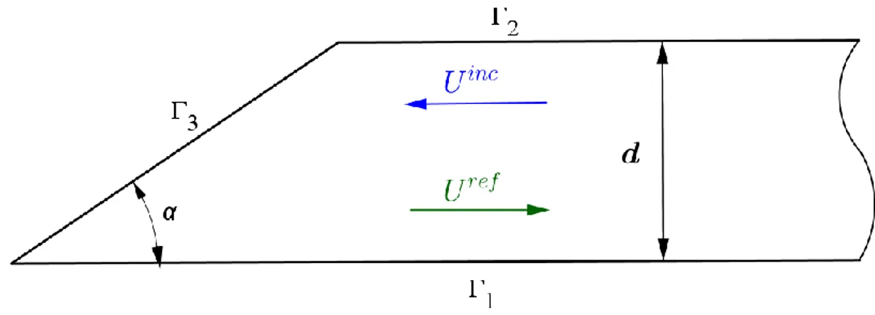
3.1 The plate structure geometry showing incident and reflected waves ... ... 40
3.2 Partitioned wedge-plate regions and common fictitious boundary... ... 40
3.3 Maximum value of radius r ... ... 41
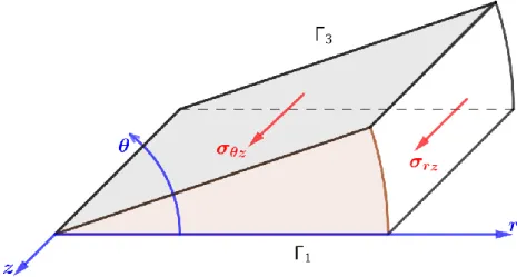
3.4 Stresses in polar coordinates in region II ... ... 43
3.5 The y-variation of displacement for the first two symmetric and antisymmetric SH modes ... 45
3.6 Plate structure with normal free end ... ... 52
3.7 Partitioned wedge-plate regions and common fictitious boundary... ... 53
List of figures
xiv
4.2 R versus normalized frequency for selected beveled edge m0 30 ... ... 60
4.3 R versus normalized frequency for selected beveled edge m0 45 ... ... 60
4.4 R versus normalized frequency for selected beveled edge m0 60 ... ... 61
4.5 R versus normalized frequency for selected beveled edge m1 30 ... ... 62
4.6 R versus normalized frequency for selected beveled edge m1 45 ... ... 63
4.7 R versus normalized frequency for selected beveled edge m1 60 ... ... 63
4.8 R versus beveled edge angle for normalized frequency m0 1.5 ... ... 64
4.9 R versus beveled edge angle for normalized frequency m0 3.5 ... ... 65
4.10 R versus beveled edge angle for normalized frequency m0 5.5 ... ... 66
4.11 R versus beveled edge angle for normalized frequency m1 1.5 ... ... 66
4.12 R versus beveled edge angle for normalized frequency m1 3.5 ... ... 67
List of tables
xv
List of tables
1.1 Analogy between operation of the human nervous system and structure SHM .... 4 4.1 Calculated results of Rm0 for particular frequencies and beveled edge 60 .... 61
4.2 Calculated results of Rm1 for particular frequencies and beveled edge 60 ... 63
4.3 Calculated results of Rm0 for particular angles and normalized frequency 1.5 65
4.4 Calculated results of Rm1 for particular angles and normalized frequency 1.5 67
Chapter 1
Chapter 1: General Introduction
2
Chapter 1
General Introduction
1.1. Motivation
Mechanical structures are widely used and indispensable in modern industry (pressure vessels, pipelines, storage tanks, ship hulls, aircraft wings, etc.). These structures are easily affected by the presence of damage mechanisms, such as corrosion or cracks which change the material properties and geometric integrity,consequently enfeebling their performance and decreasing their service life (Figure 1.1).
Chapter 1: General Introduction
3
Testing these structures is a significant issue for safety reasons and environmental impact control. Small defects are admissible as long as they are limited in size and if no overload occurs. Structural damage can continue to increase for a long time, but the ultimate failure is generally quick and unexpected. The consequences can be disastrous (structure collapse, aircraft crash, storage tank burst) (Figure 1.2). Such disasters can be predicted and avoiding such events is a good motivation for Structural Health Monitoring (SHM). This technique is rapidly emerging as a critical tool for continuous nondestructive inspection. It is used to evaluate material properties, components, or entire process units.
Figure 1.2: Incident of Aloha Airlines, Flight 243
In a typical SHM process, sensors are permanently installed to enable periodic assessment of the structure damage state. It provides information for making decisions about equipment life assessment [Boukabache et al, 2014].
A Structural Health Monitoring system is a kind of imitation of the human nervous system with integrated sensors and diagnostic capabilities (Figure 1.3). The analogy between the operation of the human nervous system and structure SHM is represented as follow, (Table 1.1):
Chapter 1: General Introduction
4
Table 1.1. Analogy between operation of the human nervous system and structure SHM
Human Nervous system Structural Health Monitoring system
More nerves around critical organs More sensors around critical parts
Pain indication Damage indication
The brain checks the intensity of the pain
and judges when to go to the doctor. The SHM system checks the structure and evaluate the reexamination actions for maintenance.
Figure 1.3: Analogy between the operation of the human nervous system and of SHM of a structure [Boukabache et al, 2014].
To improve the performance of structures monitoring, and reduce the operational cost at the same time, many researchers explored recently some new kind of structural health monitoring systems.
One of these SHM techniques is the employment of guided waves which proved to be useful in locating various types of defects in both plates and tubes. Guided waves refer to mechanical (or elastic) waves that propagate in a bounded medium parallel to the plane of its boundary. (Figure 1.4).
Chapter 1: General Introduction
5
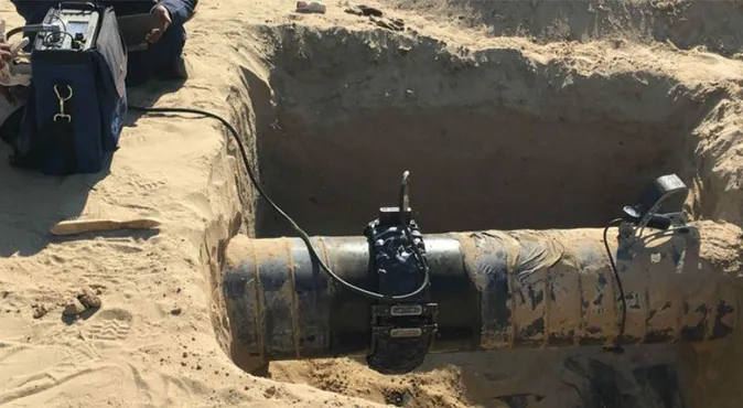
Figure 1.4: Pipeline inspection using guided wave testing (GWT)
The wave is called "guided" when it travels along the medium guided by its geometric boundaries. For this reason, the geometry has a strong influence on the behavior of the wave [Redwood, 1960]; [Rose, 1999]. Guided waves have advantages in their capacity to propagate from a single location over long distances in plates and tubes (Figure 1.5). They can offer good estimates of location, severity, and damage type, thus admitting higher efficiency, low in cost and fast detection of defects in large area of the structures [Staszewski et al, 2004]; [Croxford et al, 2007]; [Annamaria, 2016].
Chapter 1: General Introduction
6 The benefit of guided waves can also include:
High percentage coverage throughout the thickness of the structure
Ability of inspection of hidden and inaccessible regions of the structure
Inspection of underwater structures, coatings, insulation and concrete.
Avoidance of removal/reinstatement of insulation or coatings.
Guided waves can potentially be used for plate inspection such as airplane fuselage and wings often made of aluminum sheets. These sheets are assembled from holes by fasteners, which are sources of stress concentration and crack formation. The interaction of guided elastic waves with discontinuities in the structures has been the subject of scientific research of many scholars. Discontinuities in structures can be either geometrical or due to material property changes.
The complexity of such physical phenomenon fascinated many scientists over several years and has not been explained for all possible cases encountered in real situations [Demma, 2003]. Generally, the solution to such problems presents a very redoubtable challenge. A correct understanding of the physical and mathematical principles of the discontinuity effect in the structure is essential for effective utilization of these guided waves.
An important class of guided waves is the horizontal shear waves known as SH waves. The particle motion of SH waves is polarized parallel to the plate surface and perpendicular to the direction of wave propagation. These waves remain confined inside the walls of the structure and hence can travel over vast distances without energy loss (Figure 1.6).
Chapter 1: General Introduction
7
Figure 1.6: SH wave in a plate
On the other hand, the properties of the fundamental wave mode (SH0) make them very convenient for the inspection of the structure with good capability to detect defects. For those reasons, SH guided waves have the potential to be used for Non-Destructive Testing (NDT) and have recently attracted considerable interest in the structural health monitoring community [Adams, 2007] ; [Kamal and Giurgiutiu, 2014] ; [Castaings, 2014].
For the purpose of NDT studies, it is essential to model the SH wave propagation and interaction with defects analytically. This allows prediction of the repercussions of these defects on wave propagation. The knowledge of SH wave interaction with specific geometrical features can also help in the selection of incident modes and frequencies that improve inspection to various discontinuities. In the simplest case, one-single incident wave mode is used, after that it can be converted to other reflected modes in order to satisfy boundary conditions. The determination of reflection and transmission coefficients from discontinuities of different kinds has been studied by many scholars. Several approaches were proposed. The first is the development of numerical methods and tools to simulate the phenomena. The second is the development of appropriate experimental methods and techniques allowing verification and validation results of numerical simulations.
Chapter 1: General Introduction
8
For numerical methods, different approaches were investigated as methods based on wave expansion (mode-matching ) methods [Chen et al, 2015] ; [Ditri, 1996]; [Nakamura et al, 2012]; [Ahmad and Gabbert, 2012]; [Chancellier et al, 2002], finite element methods [Rajagopal and Lowe, 2007]; [Ratassep et al, 2008] ;[Koshiba et al, 1987]; [Lowe and Diligent, 2002]; [Demma et al, 2003]; [Gunawan and Hirose, 2004], or a combination of finite element formulations with waves function expansion technique [Annamaria, 2016]. Unfortunately, the study of the effects of multiple angles representing the direction of discontinuities was not widely analyzed. For these raisons, a better understanding of the interaction of guided SH waves with a beveled free end in a plate is needed.
The aim of this thesis is to develop an analytical and numerical model for SH guided wave propagation in an isotropic plate with a beveled free end. Applying these proposed procedures, the interaction between the guided waves and edge defects is well analyzed. [Mohammedi et al, 2019] The background literature on the different issues is presented in the following section.
1.2. Previous work
Although experimental observations of dynamic edge phenomenon in elastic waveguides took place over 70 years ago, the reflection of guided waves from the free end of an elastic layer remains an active area of research. Lawrie et al. [Lawrie and Kaplunov, 2012] provided a detailed review of the field that covered the period from 1958 to 2008. Within this context, a follow-up report was made by Deckers et al. [Deckers et al, 2014] in which they discussed and summarized research on wave-based methods.
Researchers have made tremendous advancements utilizing mode and frequency selections to solve many problems; for example, in the testing of pipes, rails, plates, ship hulls, and aircraft integrity [Giurgiutiu, 2007]; [Pujol, 2003]; [Rose, 2014]. In recent years, the inspection of irregularities and defects such as cracks have been carried out using horizontally polarized shear (SH) waves
Chapter 1: General Introduction
9
generated and detected by electromagnetic-acoustic transducers [Rose, 2000]; [Gao and Lopez, 2010]; [Hirao and Ogi, 1999].
The study of scattering problems varies from classical approaches such as mode matching and variational techniques to numerical techniques such as finite element and boundary element approaches, or a combination of numerical formulations with a wave function expansion technique. Among these, Abduljabbar et al. [Abduljabbar et al, 1983] studied the diffraction of SH waves in a plate with arbitrary defects by employing a finite element formulation and wave function expansion technique. Furthermore, Chen et al. [Chen et al, 2015] studied the SH guided waves propagated in a tapered plate using eigenmode matching theory and finite element methods. Ditri [Ditri, 1996] dealt with the scattering of guided elastic SH waves from material and geometric waveguide discontinuities. Nakamura et al. [Nakamura et al, 2012] studied the mode conversion behavior of an SH guided wave in a tapered plate. They investigated the different mode conversion phenomenon for abrupt and gradual thickness changes.
Many investigations have been made to study the beveled end of plates using Lamb waves. A semi-analytical finite element method has been used to simulate Lamb wave reflections at plate edges [Ahmad and Gabbert, 2012]. The Lamb wave conversion due to the beveled free end of plates has been studied theoretically as well as numerically, using the finite element method [Chancellier et al, 2002]; [Mofakhami and Boller, 2008]. Chancellier et al. used a collocation method on the beveled free end to determine the Lamb wave amplitudes and edge resonance [Chancellier et al, 2005].
Several experimental works have been published on the reflection of Lamb waves by the free and beveled edge of a plate [Castaings et al, 2002]; [Morvan et al, 2003]; [Chancellier et al, 2004]; [Santhanam and Demirli, 2013]. In these papers, the mode conversions were examined in detail over an extensive frequency range, and the energy conversion coefficients were obtained both numerically (finite element method) and experimentally.
Chapter 1: General Introduction
10
1.3. Scope and objectives
The aim of this thesis is to contribute to the understanding of SH wave propagation in an elastic plate with edge defects. The method of separation of variables (also known as the wave function expansion) is used to investigate the interactions of SH waves with the beveled free end of an elastic plate. The plate is divided into two non-overlapping regions with a common interface. Each region admits a separable solution of the corresponding wave equation. The total solution is assembled by enforcing continuity conditions at the interface. The solution preserves the total incident energy to within a small tolerance. The convergence of the solution is met when the difference between the total incident energy and reflected energy is less than 0.001% which is a very tight criterion compared to existing convergence criteria reported in many works available in the literature [Abduljabbar et al, 1983]; [Ditri, 1996]; [Morvan et al, 2003]; [Chancellier et al, 2005]. The solution provided here is compared with the known solution for a plate with a vertical end [Giurgiutiu, 2007]; [Rose, 2014].
Finally, very good agreement between the proposed numerical approach and analytical solution is observed. This indicates the effectiveness of the proposed approach. A wide range of beveled angles and incident frequencies is studied and reported here [Mohammedi et al, 2019].
1.4. Thesis outline
This thesis is divided into five chapters. The present chapter is intended to provide a general introduction to the subject, research backgrounds and useful information.
The second chapter presents a literature review of the theoretical fundamentals of wave propagation, which gives all the research background and useful information about this thesis. Guided waves in elastic plates are then introduced with particular attention on SH waves which are used in this study.
Chapter 1: General Introduction
11
Chapter 3 describes the analysis of SH waves propagating in a beveled free end plate. A region matching technique is applied to derive a series solution. Appropriate wave functions are employed to describe the displacement field. The unknown coefficients are determined by the enforcement of the continuity of displacements and stresses at the fictitious common boundary. The particular case of a plate with vertical edge is used in order to test the numerical results obtained in chapter 4
Chapter 4 deals with the numerical results of the reflecting SH waves in terms of the ratio between the energy of the mth reflected mode and the energy of
the qth incident mode. Beveled angles ranging from 20° to 90° with 0.1° increment
and normalized frequencies ranging from 0 to 5.5 are considered. The validity and accuracy of the results are checked by satisfaction of the energy conservation principle. The energy ratios are plotted as function of the beveled angles and normalized frequencies. After all, a comparative study between different approaches mentioned in the literature is done and shows the novelty of this work
In the last chapter, conclusion is provided on the findings of this thesis and additional topics that will be the subject of future work are proposed.
Chapter 2
Chapter 2 Background and literature review
13
Chapter2
Background and literature review
2.1. Introduction
In this chapter, the basic theoretical concepts for waves propagating in elastic solids on the basis of the continuum theory are described. Continuum mechanics is a classical subject that has been discussed in great generality in numerous treatises. The theory of continuous media is built upon the basic concepts of stress, motion, and deformation, upon the laws of conservation of mass, linear momentum and on the constitutive relations. The governing equations used in this thesis are for homogeneous, isotropic, linearly elastic solids. These equations are valid if it may be assumed that the strains are small and that the stress components are proportional to the strains.
The theory of wave propagation in solids is well developed and dates back to the early 1800s with the discovery of dynamical equations and waves in solids by Cauchy [Cauchy, 1822], Poisson [Poisson, 1829] and Lamé [Lamé, 1852]. During that time, these studies were merely an extension of the theory of elasticity. Poisson was the first to recognize that elastic disturbance was in general composed of two types of fundamental waves (dilatational and equivoluminal ones).
The linear theory of elasticity is based upon a linear approximation (geometrical and physical). Although it does not give an exact description of dynamics, it does provide a handy solution that is applicable as long as the assumptions are valid. This linear theory is the subject of many classic texts. A famous work entitled Mathematical Theory of Elasticity by A. E. H. Love [Love, 1906] was published in 1892 and has been reprinted many times until 1944. Numerous objects, such as an elastic 3D medium, a half space, waveguides, etc. were being studied. A wide range of waves was described, and particular
Chapter 2 Background and literature review
14
mathematical methods for analysis were derived. In recent years several books have appeared specifically dealing with wave propagation in linearly elastic solids. We mention the books presented by Kolsky [Kolsky, 1963], Achenbach [Achenbach, 1973], Whitham [Whitham, 1974], Graff [Graff, 1991], and Miklowitz [Miklowitz, 1980]. These books have summaries of the relevant elastodynamic theory. This theory is essential to the development of the method of wave propagation in plates developed in later sections.
2.2. Fundamental equations of elastodynamics
The theory to be introduced in this section attempts to deal with problems from a more fundamental basis (The dynamic theory of elasticity, called elastodynamics). The significant aspects of the theory needed for a basic understanding are presented to pursue the study in the upcoming chapters.
2.2.1. Tensor notation
Elastodynamics deals with physical quantities which are independent of any particular coordinate system that may be used to describe them. At the same time, these physical quantities are very often specified most conveniently by referring to an appropriate system of coordinates. Mathematically, such quantities are represented by Tensor. Tensor notation permits a compact expression to be written for the equations of mathematical physics that also indicates the form natural laws should take. Both indicial notation and vector notation are used in this thesis. In a Cartesian coordinate system with coordinates denoted by xi, the vector u x t( , ) is presented by
1 1 2 2 3 3
uu e u e u e (2.1)
Where, e ii ( 1, 2,3) are a set of orthonormal base vectors. Since summations of
the type (2.1) occur frequently, it is convenient to introduce the summation
convention, whereby a repeated index means summation over all values of that
Chapter 2 Background and literature review
15
i i
uu e (2.2)
The repeated index is called a dummy index because it can be replaced by any othersymbol that has not already been used in that expression. Thus, the expression in equation (2.2) can also be written as
i i j j m m
uu e u e u e (2.3)
Similarly we may have a set of nine quantities such as aij ( ,i j1, 2,3). Use will be
made of Kronecker delta defined as
1 for , 0 for , ij i j i j (2.4)
Permutationsymbol is defined as follows:
1, , , 1, 2, 3, 1, , , 1, 2, 3, 0, ijk i j k i j k
if arean even permutation of
if arean odd permutation of
otherwise.
(2.5)
The following notation is used for the field variables: Position vector x (coordinates xi)
Displacement vector u (components ui)
Strain tensor E (components ij) Stress tensor (components ij)
It may generally be assumed that the functions u x ti( , )i are differentiable. A
shorthand notation for the nine partial derivatives is
, i i j j u u x (2.6)
Chapter 2 Background and literature review
16
where the comma denotes partial differentiation with respect to the Cartesian coordinates xj.
It can be shown that the ui j, are the components of a second order tensor. A time derivative is often indicated by a dot over the quantity, i.e., i
i u u t 2.2.2. Displacement
Displacement characterizes vibrations, is a distance of a particle from its position of equilibrium. The field defining the displacement at position x at time
t is denoted by the displacement vector u x t( , )
1 1 2 2 3 3
( , ) ( , ) ( , ) ( , ) i( , ) i
u x t u x t e u x t e u x t e u x t e (2.7)
2.2.3. Strain
As a direct implication of the notion of a continuum, the deformation of the medium can be expressed in terms of the gradients of the displacement vector.
( ) ( ) ( ) i ( ) i i j i i j u x u x x u x x u x u x (2.8)
Therefore, in the first order assumption
, ,
, ,
( ) 1 1 2 2 1 1 ( ) 2 2 j j i i i i j j j j j i j i i j j i j i j j i j ij ij j u u u x u u u x x x x x x x x u u x u u x x (2.9)Where the symmetric part of (2.9)
, ,
1 2
ij ui j uj i
(2.10)
is the linear strain tensor and the skew symmetric part
, ,
1 2
ij ui j uj i
Chapter 2 Background and literature review
17
is the linear rotation tensors, which contain the spatial derivatives of the displacement field.
2.2.4. Forces and stress
In general forces on a body may be classified into two categories:
1. Body forces: Forces acting on all elements of volume of a continuum. Examples are gravity and inertia forces. These forces are represented by the symbol pi (force per unit volume) 2. Surface forces: Forces acting on the surface of a body, resulting from
physical contact with another body.
Applied external loads induce internal forces and stresses inside a body. In three-dimensions, the stress is defined by
11 12 13 21 22 23 31 32 33 ij , (2.12)
which is a second order tensor, and the first subscript indicates the surface applied and the second the direction (Figure 2.1).
Chapter 2 Background and literature review
18
Thus if a surface element has a unit outward normal n the surface traction t (stress vector) is introduced, defining a force per unit area. The surface tractions generally depend on the orientation of n as well as the locationx.
n
i ij j
t n (2.13)
Equation (2.13) is the Cauchy stress formula.
2.2.5. Equations of motion
According to the principle of balance of linear momentum, the instantaneous rate of change of the linear momentum of the body is equal to the resultant external force acting on the body at a particular instant of time. In the linear theory, this leads to the equations.
,
ij j pi ui
(2.14)
where is the mass density per unit volume.
Equations (2.14) are known as Cauchy equations of motion. For the linearized theory, the balance of moment of momentum yields the result ij ji, i.e., the stress tensor is symmetric.
2.2.6. Stress-strain relation
Assuming that the material is linearly elastic and that only small deformations are present in the domain, the linear relation between the components of the stress tensor and the components of the strain tensor is
ij Cijkm km
(2.15)
which is known as the generalized Hooke’s law.
In (2.15) Cijkm is a fourth-order tensor containing 81 elastic constants or matrix components that define the elastic properties of the material in the anisotropic medium. However, due to the symmetry of both the stress and strain tensors, there are at most 36 distinct elastic constants. Through strain energy
Chapter 2 Background and literature review
19
considerations, it follows that Cijkm Ckmij, so that even in the case of anisotropy the number of constants can be reduced to 21. The assumption of isotropy reduces the number of independent elastic constants to just 2. In summary for an isotropic, continuous medium, the elastic constant tensor can be reduced to the following:
( )
ijkm ij km ik jm im jk
c (2.16) Equation (2.16) contains two elastic constants and , which are known as Lamé’s elastic constants, which are related to the Young’s modulus E and the Poisson ratio
as , (1 )(1 2 ) 2(1 ) E E (2.17)Since the material is homogeneous, and are independent of x. The Lamé constant is also identified as the shear modulus, which is often denoted G . The stress-strain relationship (2.15) simplifies to
2
ij ij kk ij
(2.18)
which is known as the Hook’s law for isotropic elastic behavior.
2.2.7. Navier equations
The system of equations governing the motion of a homogeneous, isotropic, linearly elastic solid consists of Cauchy equations of motion, Hooke’s law and the displacement relations [Rose, 2014]; [Achenbach, 1973]. The strain-displacement relations (2.10) may be substituted into Hooke’s law (2.18) and the result in turn substituted into the stress equation of motion (2.14) to produce the governing equations
, ( ) ,
i jj j ji i i
u u p u
Chapter 2 Background and literature review
20
Motion equations (2.19) containing only particle displacements (displacement vector ui) are displacement-type partial differential equations known as Navier equations and represent three equations in Cartesian notation
2 2 2 2 2 2 2 2 2 2 2 2 2 2 2 2 2 2 2 2 2 2 ( ) ( ) ( ) y x x x x z x x y y y x y z y y y x z z z u u u u u u u p x y z x x y z t u u u u u u u p x y z y x y z t u u u u u x y z z x y 2 2 z z z u u p z t (2.20)
In vector notation equation of motion (2.19) becomes
2
( )
u u p u
(2.21)
2.3. Elastic waves in unbounded media
Elastic waves are mechanical waves propagating in an elastic medium as an effect of forces associated with volume deformation (compression and extension) and shape deformation (shear) of medium elements [Pujol, 2003]. The solution of the equation of motion for an elastic medium results in the existence of elastic waves in its interior. The wave phenomenon is a way of transporting energy without transport of matter. The propagation of energy is, then, an essential aspect of wave propagation.
2.3.1. Dilatational and rotational wave equations
Elastic homogeneous medium is considered so that the elastic moduli are constant throughout the body. In this context, the body forces are to be neglected. Navier’s equations in the absence of body forces are
, ( ) ,
i jj j ji i
u u u
(2.22)
Taking the divergence of equation (2.22) yield the scalar equation
, ( ) , ,
i jji j jii i i
u u u
Chapter 2 Background and literature review
21
which after substitution and reordering of terms involving repeated indices yields
, ( ) , ,
k iik k kii k k
u u u
or (2 ) ,ii
with the cubic dilatation uk k, , this equation is rewritten as
, 2 1 ii p c or 2 2 2 2 1 i i p x x c t (2.23) where 2 p c (2.24)
is the speed of propagation of such dilatational waves, known as the
dilatational wave speed. From (2.23), the cubic dilatation satisfies the wave
equation, known as the dilatational wave equation. The Dilatational waves are frequently called longitudinal waves, or irrotational waves, or in seismology,
P-waves (where P stands for pressure).
Navier equations (2.22) admit another wave-type solution. Taking the rotational of equation (2.22) yields the three equations
, ( ) , ,
ijkuk llj ijkul lkj ijkuk j
(2.25)
Here ijk is the permutation symbol defined in (2.5). The term ul lkj, is
symmetric in the indices j and k, whereas the permutation symbol ijk is antisymmetric. Hence, the second term appearing in equation (2.25) vanishes. Making use of this result, equation (2.25) reduces to
, 2 1 i jj i s w w c or 2 2 2 2 1 i i j j s w w x x c t (2.26) where s c (2.27)
Chapter 2 Background and literature review
22
is the shear speed. Equation (2.26) is the three-dimensional wave equation known as transverse waves, or shear waves, or S-waves. The quantity wi is the vector rotation of the displacement field
, 1 1 2 2 i ijk k j ijk kj w u W , 1( , ,) 2 ij i j j i W u u (2.28)
Here W is the skew-symmetric part of the displacement gradient ij uk j,
known as the infinitesimal rotation tensor.
2.3.2. Helmholtz representation
The results presented in the previous section can also be found in an alternative way known as Helmholtz decomposition. The vector field ui can be expressed as the sum of the gradient of a scalar field vi and the curl of a vector field (divergence-free) wi , , i i i i ijk k j u v w H or u H (2.28) and , 0 k k H or H 0 (2.29)
Direct calculation show that ui i, 0 and ijk k jv , 0. In other words, ui has been decomposed into the sum of an irrotational vector vi and a solenoidal vector wi. The case where ui is solenoidal (vi 0) and ui wi, Navier’s equations (2.25)
reduce to , i jj i u u (2.30)
which is the wave equation governing shear waves or equivoluminal waves. The case where the displacement is irrotational (wi 0) and ui vi, can be found by
Chapter 2 Background and literature review 23 , 2 i jj i u u (2.31)
which is the dilatational wave equation. Consequently, an arbitrary displacement can be regarded as the sum of equivoluminal and dilatational waves. Equations (2.30) and (2.31) are independent of each other, which mean that the longitudinal and shear waves propagate without interaction in unbounded media.
2.4. Guided waves
In comparison, a bulk wave travels in an infinite media, for which boundaries do not influence wave propagation. Hence they travel in the bulk of the material. Guided waves are waves that propagate within the boundaries of a structure. The boundaries not only influence the propagation but they guide the wave along the structure. Bulk and guided waves are governed by the same set of partial differential equations. The difference in mathematical solution is that guided waves must satisfy some additional boundary conditions [Giurgiutiu, 2007]. The difficulty in the application of guided waves arises from the complexity of the solution. Guided waves are characterized by an infinite number of modes associated with a given partial differential equation solution. The basic principles of guided waves are very well known, and several textbooks discuss the topics [Giurgiutiu, 2007]; [Graff, 1991]; [Brekhovskikh, 1980].
In this thesis, the guided waves propagation in plates will be considered.
2.4.1. Guided waves in plates
The elastic wave propagation theory in plates has been built-up over one hundred years. The propagation of waves in isotropic plates with free boundary conditions was first studied by Lamb [Lamb, 1917] after whom the guided waves in free plates are named. His study analyzed symmetric and anti-symmetric modes separately. In 1945 Rayleigh and Lindsay investigated the wave propagation in isotropic plates with free boundary conditions [Rayleigh and Lindsay, 1945]. In their works, the Rayleigh-Lamb equations were developed, which identified the relationship between wave frequency and wave number
Chapter 2 Background and literature review
24
under certain conditions. A comprehensive analysis and contribution to the understanding of guided waves in plates were given by Victorov [Victorov, 1970], Achenbach [Achenbach, 1973], Graff [Graff, 1991], Rose [Rose, 2014] and Royer and Dieulesaint [Royer and Dieulesaint, 2000]. Some examples of guided wave problems that have been solved and whose solution has inherited the name of the investigator are Rayleigh waves, Lamb waves, Love waves, and Shear horizontal waves. A brief description is listed as follows:
2.4.1.1 Rayleigh waves
Rayleigh waves, as the most straightforward wave, propagate on the free surface of a semi-infinite solid [Ostachowicz et al, 2011]. In these waves, the particle motion is composed of elliptical movements in the x y vertical plane and of motion parallel to the direction of propagation x(as shown in Figure 2.2). The motion amplitude decreases rapidly with depth y starting from the wave crest. The Rayleigh waves are very sensitive to surface defects with very little penetration in the depth of the solid [Hirao and Ogi, 1999]. For this reason, they can be used to inspect the surface properties for a structure.
Figure 2.2: Rayleigh wave [Ostachowicz et al, 2011].
2.4.1.2 Lamb waves
Lamb waves are waves that are guided between two parallel free surfaces, such as the upper and lower surfaces of a plate (Figure 2.3). These waves can
Chapter 2 Background and literature review
25
only be generated in thin-walled structures so that the motion amplitude remains the same on both top and bottom surfaces only. Therefore Lamb waves are of two basic varieties, symmetric Lamb-waves modes and antisymmetric Lamb-wave modes [Hirao and Ogi, 1999]; [Ostachowicz et al, 2011]. Unlike the Rayleigh waves, the Lamb waves are highly dispersive, and their speed is related to their frequency and plate thickness.
Figure 2.3: Lamb wave [Ostachowicz et al, 2011].
2.4.1.3 Love waves
Love waves are another kind of surface waves applied for surface inspection. These waves were firstly found by Love in 1911 and verified by many researchers. Their particle motion is horizontal (in the x z plane) and perpendicular to the direction of propagation x. As in the case of Rayleigh waves, their wave amplitude decreases rapidly with depth (Figure 2.4).
Chapter 2 Background and literature review
26 2.4.1.4 Shear horizontal waves
Shear horizontal (SH) waves are characterized by particle motion maintained in the x z horizontal plane, as their name explained. The direction of the particle motion is perpendicular to the direction of wave propagation x (Figure 2.5). The SH waves can be symmetric and antisymmetric. Except for the very fundamental mode, the SH wave modes are all dispersive. The advantage of applied SH waves on structural health monitoring is summarized by Petcher et al. [Petcher et al, 2013].
Figure 2.5: Horizontal shear wave [Ostachowicz et al, 2011].
2.4.2. Shear horizontal wave in plate
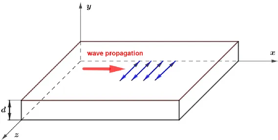
Shear horizontal waves have a particle motion contained in a plane parallel to the surface of the plate ( x z ). The axes definition is shown in Figure 2.6. The x axis is placed along the direction of wave propagation, whereas the
z
axis is perpendicular to it. [Giurgiutiu, 2007]Chapter 2 Background and literature review
27
Figure 2.6: Particle motion and coordinate definition for SH plate waves [Giurgiutiu, 2007].
2.4.2.1 General equation
The SH mode can be considered as the superposition of waves reflecting from the upper and lower surfaces of the plate, polarized horizontally (in the
z
axis direction). The problem is assumed to be z-invariant, i.e., ( ) 0z
. Particle
motion has only a Uz component and if Uz is independent of
z
, then equation(2.26) reduces to: 2 2 1 z z s U U c or 2 2 2 2 2 2 2 1 z z z s U U U x y c t (2.32) where Uz w3
It is assumed that the particle motion has the form
, , i kx t
z
U x y t f y e (2.33)
This form of the solution is chosen because it represents a wave motion propagating in the x direction (due to the exponential term i kx t
e ) and has a fixed distribution in the y direction (standing waves across the thickness d ). Notice that Uz is independent of
z
, so that the problem is assumedz
-invariant.Chapter 2 Background and literature review
28
Substitution of equation (2.33) into equation (2.32) and division of both sides by
i kx t e yields
2 2 2 2 2 0 s f y k f y x c (2.34)The solution of equation (2.34) has the general form
sin
cos
f y A y B y (2.35) Where is defined as 2 2 2 2 s k c (2.36)and A,B are arbitrary constants. The general form of the displacement field is therefore
, , sin cos i kx t
z
U x y t A y B y e (2.37)
The boundary conditions state that the upper and lower plate surfaces are traction free
, ,
z
, ,
0 yz U x d t x d t y (2.38)Without going into details [Giurgiutiu, 2007], Boundary conditions (2.38) lead to the dispersion equations characterized by the system of linear homogeneous equations with the determinant
sin d cos d 0 (2.39)
Equation (2.39) is the characteristic equation of SH wave modes and is zero when either:
sin d 0 (2.40)
Chapter 2 Background and literature review
29
cos d 0 (2.41)
which corresponds to antisymmetric modes (A-modes) of the SH waves. By virtue of the simplicity of the solution, explicit solutions of equations (2.40) and (2.41) are , 0, 1, 2,... , 1, 3, 5,... 2 S A d n n n d n (2.42) The values S d and A d
given by equations (2.42) are the Eigenvalues for symmetric and antisymmetric motions. The solutions to equations (2.40) and (2.41) can be written as
2
n
d
(2.43)
where n
0, 2, 4, ...
for symmetric SH modes and n
1, 3, 5, ...
for antisymmetricSH modes. After substitutions, the general solution (2.33) becomes
, , cos 2 i kx t S z n U x y t B ye d (2.44)for symmetric SH waves (S-modes), and
, , sin 2 i kx t A z n U x y t A ye d (2.45)For antisymmetric SH waves (A-modes).
A sketch of the symmetric SH modes (S0, S1, S2) and antisymmetric SH modes (A0, A1, A2) are illustrated in Figure 2.7.
Chapter 2 Background and literature review
30
Figure 2.7: SH waves, (a) symmetric modes, (b) Anti-symmetric modes. [Giurgiutiu, 2007].
2.4.2.2 Dispersion of SH waves
By using the definition of the wave number
p
k c
(2.46)
where c is the mode phase velocity p
The dispersion equation (2.36) can be written as
2 2 2 2 2 2 s p n c c d (2.47)
Equation (2.47) can be solved for the phase velocity c in terms of the frequency p
thickness product 2 fd (where 2 f )
2 2 2 2 2 4(2 ) p s s fd c c fd n c (2.48)
It should be noted that when n0, corresponding to the first symmetric mode
SH0 , the phase velocity cp is equal to cs, so the SH0 wave mode is not dispersive and propagates at the shear wave speed cs. For all other SH modes (n0) the
phase velocity is varying with the frequency-thickness product. This phenomenon is called dispersion, and results in the distortion of the shape of the wave packet
Chapter 2 Background and literature review
31
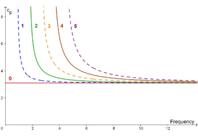
containing multiple frequencies that propagates for long distances. The first five SH modes of the phase velocity dispersion curves over a frequency thickness range of 0-14 MHz-mm, are plotted in Figure 2.8. The solid and dashed curves represent the symmetric and antisymmetric modes respectively.
The cutoff frequencies of the SH modes which correspond to infinite phase velocities can be found by setting the denominator in equation (2.48) equal to zero. The nth cutoff frequency is given by
2
2 s n nc fd (2.49)It should be noted that , even integer n represents symmetric modes and odd integer n represents antisymmetric modes.
Figure 2.8 also indicates the asymptotic behavior of the phase velocity. All the SH modes converge to cs as the frequency thickness product becomes large. In this example cs 3.1mm/s for aluminum plate.
The phase velocity represents the velocity at which a mode at a given frequency is traveling in a medium. If this mode is dispersive, then the group velocity is associated with the propagation velocity of a group of waves of similar frequency.
Chapter 2 Background and literature review
32
Figure 2.8: Phase velocity dispersion curves for SH modes.
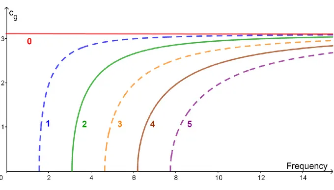
The group velocity corresponds to the velocity at which the energy of a multi frequency wave packet is traveling.
Solving the dispersion equation for the quantity d cg dk
(by definition, the group
velocity ), it can be shown [Rose, 1999], that the group SH wave velocities can be expressed as : 2 2 2 1 2 g s s n c c fd c (2.50)
Chapter 2 Background and literature review
33
Figure 2.9: Group velocity dispersion curves for SH modes.
Notice that at cutoff frequencies given by equation (2.49), the group velocity of any mode is zero. As fd approaches infinity for any mode, the group velocity approaches the shear wave cs. Plots of SH mode group velocity curves are illustrated in Figure 2.9.
2.5. Wave equation in cylindrical and polar coordinates
While Cartesian coordinates are attractive because of their simplicity, there are many problems in mechanics fruitfully analyzed when they are modeled as having particular geometry and various symmetries, such as cylindrical symmetry. When looking for waves with some chosen geometry, it is advantageous to get at the solutions to the wave equation directly in these coordinates.
2.5.1. Transforming the wave equation


![Figure 2.6: Particle motion and coordinate definition for SH plate waves [Giurgiutiu, 2007]](https://thumb-eu.123doks.com/thumbv2/123doknet/14897157.652043/44.892.270.663.122.402/figure-particle-motion-coordinate-definition-plate-waves-giurgiutiu.webp)
![Figure 2.7: SH waves, (a) symmetric modes, (b) Anti-symmetric modes. [Giurgiutiu, 2007]](https://thumb-eu.123doks.com/thumbv2/123doknet/14897157.652043/47.892.166.790.135.384/figure-waves-symmetric-modes-anti-symmetric-modes-giurgiutiu.webp)