DOI 10.1515 / ADVGEOM.2010.001 de Gruyter 2010
Secant dimensions of low-dimensional
homogeneous varieties
Karin Baur
∗and Jan Draisma
†(Communicated by R. Miranda)
Abstract. We completely describe the higher secant dimensions of all connected homogeneous projective varieties of dimension at most 3, in all possible equivariant embeddings. In particular, we calculate these dimensions for all Segre–Veronese embeddings of P1× P1
, P1× P1 × P1
, and P2× P1, as well as for the flag variety F of incident point-line pairs in P2. For P2× P1and F the results are new, while the proofs for the other two varieties are more compact than existing proofs. Our main tool is the second author’s tropical approach to secant dimensions.
1
Introduction and results
Let K be an algebraically closed field of characteristic 0; all varieties appearing here will be over K. Let G be a connected affine algebraic group, and let X be a projective variety on which G acts transitively. An equivariant embedding of X is by definition a G-equivariant injective morphism ι : X → P(V ), where V is a finite-dimensional (rational) G-module, subject to the additional constraint that ι(X) spans P(V ).
The k-th (higher) secant variety kι(X) of ι(X) is the closure in P(V ) of the union of all subspaces of P(V ) spanned by k points on ι(X). The expected dimension of kι(X) is min{k(dim X + 1) − 1, dim V − 1}; this is always an upper bound on dim kι(X). We call kι(X) non-defective if it has the expected dimension, and defective otherwise. We call ι non-defective if kι(X) is non-defective for all k, and defective otherwise.
We want to compute the secant dimensions of ι(X) for all X of dimension at most 3 and all ι. This statement really concerns only finitely many pairs (G, X): Indeed, as X is projective and G-homogeneous, the stabiliser of any point in X is parabolic (see [2, §11]) and therefore contains the solvable radical R of G. But then R also acts trivially on the span of ι(X), which is P(V ), so that we may replace G by the quotient G/R, which is semisimple. In addition, we may and shall assume that G is simply connected. Now V is
∗The first author is supported by EPSRC grant number GR/S35387/01. †The second author is supported by DIAMANT, an NWO mathematics cluster.
an irreducible G-module, and ι(X) is the unique closed orbit of G in PV , the cone over which in V is also known as the cone of highest weight vectors. Conversely, recall that for two dominant weights λ and λ0the minimal orbits in the corresponding projective spaces PV (λ) and PV (λ0) are isomorphic (as G-varieties) if and only if λ and λ0have the same support on the basis of fundamental weights. So, to prove that all equivariant embeddings of a fixed X are non-degenerate, we have to consider all possible dominant weights with a fixed support.
Now there are precisely seven pairs (G, X) with dim X ≤ 3, namely (SLi2, (P1)i)
for i = 1, 2, 3, (SL3, P2), (SL3× SL2, P2 × P1), (SL4, P3), and (SL3, F ), where F is
the variety of flags p ⊂ l with p, l a point and a line in P2, respectively. The
equivari-ant embeddings of Pi for i = 1, 2, 3 are the Veronese embeddings; their higher secant
dimensions — and indeed, all higher secant dimensions of Veronese embeddings of pro-jective spaces of arbitrary dimensions — are known from the work of Alexander and Hirschowitz; see [1] or [3]. In low dimensions there also exist tropical proofs for these results: P1and P2 were given as examples in [10], and for P3see the Master’s thesis of
Silvia Brannetti [4]. The other varieties are covered by the following theorems.
First, the equivariant embeddings of P1 × P1 are the Segre–Veronese embeddings,
parameterised by the degree (d, e) (corresponding to the highest weight dω1+ eω2where
the ωiare the fundamental weights), where we may assume d ≥ e. The following theorem
is known in the literature; see for instance [5, Theorem 2.1] and the references there. Our proof is rather short and transparent, and serves as a good introduction to the more complicated proofs of the remaining theorems.
Theorem 1.1. The Segre–Veronese embedding of P1× P1of degree(d, e) with d ≥ e ≥ 1
is non-defective unlesse = 2 and d is even, in which case the (d + 1)-st secant variety has codimension1 rather than the expected 0.
The equivariant embeddings of P1× P1
× P1
and of P2× P1are also Segre–Veronese
embeddings. While writing this paper we found out that the following theorem has al-ready been proved in [6]. We include our proof because we need its building blocks for the other 3-dimensional varieties.
Theorem 1.2. The Segre–Veronese embedding of P1× P1× P1 of degree(d, e, f ) with
d ≥ e ≥ f ≥ 1 is non-defective unless
(1) e = f = 1 and d is even, in which case the (d + 1)-st secant variety has codimension 1 rather than the expected 0, or
(2) d = e = f = 2, in which case the 7-th secant variety has codimension 1 instead of the expected0.
The remaining two theorems are newer.
Theorem 1.3. The Segre–Veronese embedding of P2× P1of degree(d, e) with d, e ≥ 1
is non-defective unless
(1) d = 2 and e = 2k is even, in which case the (3k + 1)-st secant variety has codimen-sion3 rather than the expected 2 and the (3k + 2)-nd secant variety has codimension 1 rather than 0; or
(2) d = 3 and e = 1, in which case the 5-th secant variety has codimension 1 rather than the expected0.
Finally, the equivariant embeddings of F are the minimal orbits in PV for any irre-ducible SL3-representation of highest weight dω1+ eω2.
Theorem 1.4. The image of F in PV , for V an irreducible SL3-representation of highest
weightdω1+ eω2withd, e ≥ 1 is non-defective unless
(1) d = e = 1, in which case the 2-nd secant variety has codimension 1 rather than 0, or (2) d = e = 2, in which case the 7-th secant variety has codimension 1 rather than 0. Remark 1.5. Most defective Segre–Veronese varieties above can be explained as follows. The Veronese varieties are rank-1 loci of so-called catalecticant matrices, whose entries are homogeneous coordinates of the ambient space [11]. The Segre product of such vari-eties is then the rank-1 locus of the Kronecker product of the corresponding catalecticant matrices. Hence the k-th secant variety of this Segre product is contained in the locus of rank-k matrices. In general this does not give much information about the ideal, but sometimes it is just enough to conclude that a secant variety that was expected to fill the space actually is contained in a hypersurface. This argument is used extensively in [7].
To the best of our knowledge Theorems 1.3 and 1.4 are new. Moreover, F seems to be the first settled case where maximal tori in G do not have dense orbits. Our proofs of Theorems 1.1 and 1.2 are more compact than their original proofs [5, 6]. Moreover, the planar proof of Theorem 1.1 serves as a good introduction to the more complicated induction in the three-dimensional cases, while parts of the proof of Theorem 1.2 are used as building blocks in the remaining proofs.
We shall prove our theorems using a polyhedral-combinatorial lower bound on higher secant dimensions introduced by the second author in [10]. Roughly this goes as follows: to a given X and V we associate a finite set B of points in Rdim X, which parameterises a certain basis in V . Now to find a lower bound on dim kX we maximise
k
X
i=1
[1 + dim AffRWini(f )]
over all k-tuples f = (f1, . . . , fn) of affine-linear functions on Rdim X, where Wini(f )
is the set of points in B where fi is strictly smaller than all fj with j 6= i, and where
AffRdenotes taking the affine span. Typically, this maximum equals 1 plus the expected dimension of dim kι(X), and then we are done. If not, then we need other methods to prove that kι(X) is indeed defective — but most defective cases above are known in the literature.
As a motivation for this optimisation problem we now carry out our proof in one particular case. For the Segre–Veronese embedding of X = P1× P1of degree (d, e) the
set B is the grid {0, . . . , d} × {0, . . . , e} ⊆ R2. Take for instance d = 3 and e = 2.
In Figure 1 the points in B are grouped into four triples spanning the plane. It is easy to see — for instance with Lemma 2.6 below — that there exist affine-linear functions f1, . . . , f4inducing this partition, so that 4X has the expected dimension 4 · 3 − 1 = 11.
1
2
3
Figure 1: The embedding Seg ◦(v3× v2) of P1× P1is non-defective.
Our tropical approach closely related to Sturmfels–Sullivant’s combinatorial secant varieties [13], Miranda–Dumitrescu’s degeneration approach (private communication), and Develin’s tropical secant varieties of linear spaces [9]. We find it very surprising and promising that strong results on secant varieties of non-toric varieties such as F can be proved with our approach.
The remainder of this paper is organised as follows. In Section 2 we recall the tropical approach, and prove a lemma that will help us deal with the flag variety. The tropical ap-proach depends rather heavily on a parameterisation of X, and in Section 3 we introduce the polynomial maps that we shall use. In particular, we give, for any minimal orbit (not necessarily of low dimension, and not necessarily toric), a polynomial paramaterisation whose tropicalisation has an image of the right dimension; these tropical parameterisa-tions are useful in studying tropicalisaparameterisa-tions of minimal orbits; see Remark 3.3. Finally, Sections 4–7 contain the proofs of Theorems 1.1–1.4, respectively.
Acknowledgments. We thank the referee for such thorough reading of the first version of this paper, and for many suggestions to improve it.
2
The tropical approach
2.1 Two optimisation problems. We recall from [10] a polyhedral-combinatorial
op-timisation problem that plays a crucial role in the proofs of our theorems; here AP abbre-viates Affine Partition.
Problem 2.1 (AP(A, k)). Let A = (A1, . . . , An) be a sequence of finite subsets of Rm
and let k ∈ N. For any k-tuple f = (f1, . . . , fk) of affine-linear functions on Rmlet the
sets Wini(f ), i = 1, . . . , k, be defined as follows. For b = 1, . . . , n we say that fiwinsb
if fiattains its minimum on Abin a unique α ∈ Ab, and if this minimum is strictly smaller
than all values of all fj, j 6= i on Ab. The vector α is then called a winning direction of
fi. Let Wini(f ) denote the set of winning directions of fi. Now the problem AP(A, k)
can be stated as follows.
Maximise Pk
i=1[1 + dim AffRWini(f )] over all k-tuples f of affine-linear functions
Note that if every Ab is a singleton {αb}, then Wini(f ) is just the set of all αb on
which fiis smaller than all other fj, j 6= i. We shall then also write AP({α1, . . . , αn}, k)
for the optimisation problem above. In this case we are really optimising over all possible regular subdivisionsof Rminto k open cells. Each such subdivision induces a partition of the αbinto the sets Wini(f ) — at least if no αblies on a border between two cells, but
this is easy to achieve without decreasing the objective function. Below we shall never explicitly construct the fj, nor the regular subdivision, but rather just give the induced
partition on the points αi, which will lie in two- or three-dimensional real space depending
on the dimension of X. The following two lemmas will be used throughout to establish the existence of the fiwithout actually constructing them.
Lemma 2.2. Let S be a finite set in Rm, letf
1, . . . , fkbe affine-linear functions on Rm,
and letg1, . . . , glalso be affine-linear functions on Rm. LetSibe the subset ofS where
fi < fj for allj 6= i, and let Tibe the subset ofS1wheregi < gj for allj 6= i. Then
there exist affine-linear functionsh1, . . . , hlsuch that
(1) hi< hjonTifori, j = 1, . . . , l and j 6= i;
(2) hi< fjonTifori = 1, . . . , l and j = 2, . . . , k; and
(3) fi< hjonSifori = 2, . . . , k and j = 1, . . . , l.
In other words, the functionsh1, . . . , hl, f2, . . . , fk together induce the partitionT1, . . . ,
Tl, S2, . . . , SkofS.
Proof. Take hi= f1+ εgifor ε positive and sufficiently small. 2
This lemma implies, for instance, that one may find appropriate Wini(f ) (still for
the case of singletons Ab) by repeatedly cutting polyhedral pieces of space in half. For
instance, in Figure 1 the plane is cut into four pieces by three straight cuts. Although this is not a regular subdivision of the plane, by the lemma there does exist a regular subdivision of the plane inducing the same partition on the 12 points. The next lemma concerns the following, slightly different polyhedral optimisation problem Voronoi Partition.
Problem 2.3 (VP(S, k)). Let S be a finite set in Rm, and equip Rmwith a positive defi-nite inner product with associated norm || . ||. For any k-tuple v = (v1, . . . , vk) of points
in Rmlet Vori(v) denote the intersection of S with the open Voronoi cell of vi, i.e.,
Vori(v) := {α ∈ S | ||α − vi|| < ||α − vj|| for all j 6= i}.
Then the problem VP(S, k) can be stated as follows.
MaximisePk
i=1[1 + dim AffRVori(v)] over all k-tuples v of points in Rm; call the
maximumVP∗(A, k).
Lemma 2.4 ([10, Lemma 3.8]). Let S be a finite subset in the Euclidean space (Rm,
|| . ||), let v = (v1, . . . , vk) be a k-tuple of points in Rm for which the setsVori(v)
partitionS, that is, there are no points of S on the boundary of any Voronoi cell. Then there exists ak-tuple f = (f1, . . . , fk) of affine-linear functions on Rmwhose associated
regular subdivision partitions the setS in exactly the same parts Vori(S). In particular,
Lemmas 2.2 and 2.4 can only be applied directly to AP if the Ab are singletons,
while the Ab in our application to the 3-dimensional flag variety F are not. We get
around this difficulty by giving a lower bound on AP∗(A, k) for more general A in terms of AP∗(A0, k) for some sequence A0 of singletons. In the following lemmas a convex polyhedral conein Rm is by definition the set of non-negative linear combinations of a finite set in Rm, and it is called pointed if it does not contain any non-trivial linear subspace of Rm.
Lemma 2.5. Let A = ({α1}, . . . , {αn}) be an n-tuple of singleton subsets of Rm.
Fur-thermore, letk ∈ N, let Z be a pointed convex polyhedral cone in Rm, and letf be a
k-tuple of affine-linear functions on Rm. Then the value ofAP(A, k) at f is also attained
at somef0= (f10, . . . , fk0) for which every fi0is strictly decreasing in thez-direction, for everyz ∈ Z \ {0}.
Proof. As Z is pointed, there exists a linear function f0on Rmsuch that every fj+ f0is
strictly decreasing in the z-direction, for every z ∈ Z. But since fi(α) < fj(α) ⇔ fi(α) + f0(α) < fj(α) + f0(α)
we have Wini((fj+ f0)j) = Wini(f ) for all i, and we are done. 2
It is crucial in this proof that only values of fiand fjat the same α are compared —
that is why we have restricted ourselves to singleton-AP here.
Lemma 2.6. Let A = (A1, . . . , An) be a k-tuple of finite subsets of Rmand letk ∈ N.
Furthermore, letZ be a pointed convex polyhedral cone in Rmand define a partial order
≤ on Rmby
p ≤ q :⇔ p − q ∈ Z.
Suppose that for everyb, Abhas a unique minimal elementαb with respect to this order.
Then we have
AP∗(A, k) ≥ AP∗({α1, . . . , αn}, k)
Proof. Let d∗ = AP∗({α1, . . . , αn}, k). By Lemma 2.5 there exists a k-tuple f =
(f1, . . . , fk) of affine-linear functions on Rmfor which AP({α1, . . . , αn}, k) also has
value d∗and for which every fiis strictly decreasing in all directions in Z. We claim that
the value of AP(A, k) at this f is also d∗. Indeed, fix b ∈ B and consider all fi(α) with
α ∈ Aband i = 1, . . . , k. Because αb− α ∈ Z for all α ∈ Aband because every fiis
strictly decreasing in the directions in Z, we have fi(αb) < fi(α) for all α ∈ Ab\ {αb}
and all i. Hence the minimum, over all pairs (i, α) ∈ {1, . . . , k} × Ab, of fi(α) can
only be attained in pairs for which α = αb. Therefore, in computing the value at f of
AP(A, k) the elements of Abunequal to αbcan be ignored. We conclude that AP(A, k)
2.2 Tropical bounds on secant dimensions. Rather than working with projective va-rieties, we work with the affine cones over them. So suppose that C ⊆ Kn is a closed cone (i.e., closed under scalar multiplication with K), and set
kC := {v1+ · · · + vk | v1, . . . , vk∈ C}.
Suppose that C is unirational, and choose a polynomial map f = (f1, . . . , fn) : Km→
C ⊆ Kn that maps Kmdominantly into C. Let x = (x
i)mi=1and y = (yb)nb=1be the
standard coordinates on Kmand Kn. The tropical approach depends very much on these
coordinates; in particular, one would like f to be sparse. For every b = 1, . . . , n let Ab
be the set of α ∈ Nmfor which the monomial xαhas a non-zero coefficient in fb, and set
A := (A1, . . . , An).
Theorem 2.7 ([10]). For all k ∈ N, dim kC ≥ AP∗(A, k). Remark 2.8. In fact, in [10] this is proved provided thatS
bAbis contained in an affine
hyperplane not through 0, but this can always be achieved by taking a new map f0(t, x) := tf (x) into C, without changing the optimisation problem AP(A, k).
In Section 3 we introduce a polynomial map f for general minimal orbits that seems suitable for the tropical approach, and after that we specialise to low-dimensional varieties under consideration.
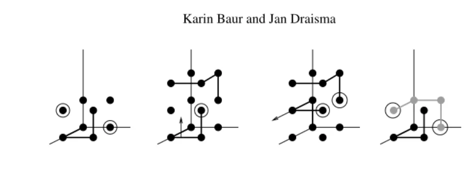
2.3 Non-defective pictures. Our proofs will be entirely pictorial: given a set B of lat-tice points in Z2or Z3according as dim X = 2 or dim X = 3, we solve the optimisation
problem AP(B, k) for all k. To this end, we shall exhibit a partition of B into parts Bi
such that there exist affine-linear functions fion R2or R3, exactly one for each part, with
Bi= Wini(f ). If each Biis affinely independent, and if moreover the affine span of each
Bihas dim X, except possibly for one single Bi, then we call the picture non-defective,
as it shows, by Theorem 2.7, that all secant varieties of X in the given embedding have the expected dimension. Otherwise, we call the picture defective.
The Bi that we shall use will have very simple shapes: in dimension 2 they will all
be equivalent, up to distance-preserving automorphisms of the lattice Z2, to the triple {0, e1, e2}, or to the edge {0, e1}, or to the single point {0}. These building blocks
also appear in dimension 3, but there we also have 3-dimensional blocks equivalent to {0, e1, e2, e3}, which we call corners, or to {0, e1, e1+ e2, e1+ e2+ e3}, which we call
snakes; see Figure 2. Only for the flag-variety F it will be convenient to use a single slightly different building block in one instance.
Figure 2: A corner (left) and a snake (right).
The fiwill not be computed explicitly, but their existence will be deduced from
Figure 3: Snakes and threats
inducing the given partition of B into the Bi, one can try and take the barycentre Mi of
each Bi as its point vi. The squared distance, relative to the standard inner product, of
this barycentre of Bito its vertices is as follows:
single point {0}: 0; edge {0, e1}: twice 1/4;
triangle {0, e1, e2}: once 2/9, twice 5/9;
corner {0, e1, e2, e3}: once 3/16, thrice 11/16; and
snake {0, e1, e1+ e2, e1+ e2+ e3}: twice 6/16, twice 14/16 (for the heads of the snake).
Given any snake Bj, there are exactly two lattice points outside Bj that also have
squared distance 14/16 from the barycentre Mj. They are indicated with a circle in the
left-most picture in Figure 3. If such a point p happens to be the head of another snake Bi, then we say that p is threatened by Bj, as it lies on the border of the Voronoi cells of
Biand Bj. It can happen that both Bjthreatens a head of Bi, and Bithreatens a head of
Bj; see the third picture in Figure 3 for an example. It is straightforward to verify that if
all blocks Bi are of the shapes above, then any lattice point p of Biis closer to Mithan
to any Mjwith j 6= i unless p is threatened by Bj in the sense above. In our pictures we
will then draw a circle around p, to indicate that it is threatened by Bj. Now our pictures
are constructed in such a way that all such threats can be removed by slightly wiggling the vifrom their initial positions Mi. For snake Bj threatening the head p of snake Bi this
can be done in more than one way: either by moving vifrom Mislightly towards p, or by
moving vjfrom Mjslightly away from p. In our pictures we indicate such wigglings with
small arrows: an arrow attached to (the edges connecting) Bi indicates that vi is moved
slightly in the direction of the arrow; see the second picture in Figure 3. This wiggling direction will always be one of the six positive or negative coordinate directions. Remark 2.9. It is admittedly somewhat cumbersome to verify that the indicated wigg-lings do indeed remove all threats. It would be nicer to have a theorem stating that any partition of a point set B in Z3 into single points, edges, triangles, corners, and snakes
is induced by some regular subdivision. However, this naive statement is not true for the simple reason that the two snakes in the rightmost picture in Figure 3 cannot be separated by a hyperplane. Now of course two such snakes can be replaced by two corners, and it might be true that any partition of B avoiding two such snakes is induced by some regular subdivision. However, we did not manage to prove anything substantial along these lines. Instead we have tried to reduce the number of threats in our pictures so that the reader can verify the pictorial proof with the following straightforward visual check: for each snake,
look at each of the two vertices that it potentially threatens. If that is the head of an other snake, one or both of the snakes should have arrows removing this threat.
In our proofs by induction we shall build defective pictures for sets B using non-defective pictures for smaller sets built earlier. To ensure that the resulting partition of B is indeed induced by some regular subdivision, one can proceed in two ways. First, if the smaller pictures can be separated by each other by a regular subdivision, e.g. by repeatedly cutting with planar cuts, then we may invoke Lemma 2.2. Occasionally, however, we shall match up redundant points from two smaller pictures to form a new building block (snake, corner, etc.). In such a situation we invoke Lemma 2.4, after checking that potential new threats created near the building block are removed by wiggling as above.
3
A polynomial map
We retain the setting of the Introduction: G is a simply connected, connected, semisimple algebraic group, V is a G-module, and we wish to determine the secant dimensions of X, the unique closed orbit of G in PV . Let C be the affine cone in V over X. Fix a Borel subgroup B of G, let T be a maximal torus of B and let vλ∈ V span the unique B-stable
one-dimensional subspace of V ; λ denotes the T -weight of vλ. In other words, vλ is a
highest weight vector and λ is the highest weight of V . Let P ⊇ B be the stabiliser in G of Kvλ(so that X ∼= G/P as a G-variety) and let U− be the unipotent radical of the
parabolic subgroup opposite to P and containing T . Let u denote the Lie algebra of U−,
let X(u) be the set of T -roots on u, and set ˜X(u) := X(u) ∪ {0}. For every β ∈ X(u) choose a vector Xβspanning the root space uβ. Moreover, fix an order on X(u). Then it
is well known that the polynomial map Ψ : KX(u)˜ → V, t 7→ t0
Y
β∈X(u)
exp(tβXβ)vλ,
where the product is taken in the fixed order, maps dominantly into C. This map will play the role of f from Subsection 2.2.
In what follows we shall need the following notation: Let XR:= R ⊗ZX(T ) be the real vector space spanned by the character group of T , let ξ : RX(u) 7→ XRsend r to P
βrββ and also use ξ for the map R ˜
X(u)→ X
Rwith the same definition; in both cases
we call ξ(r) the weight of r.
Now for a basis of V : since V is a G-module with P stabilizing the line Kvλthrough
the highest weight vector, all of V is obtained by letting the universal enveloping algebra of u act on vλ. The Poincar´e–Birkhoff–Witt (PBW) theorem tells us that for any linear
order on the basis (Xβ)β∈X(u) of u, the universal enveloping algebra of u has a basis
{Q
β∈X(u)X rβ
β | rβ ∈ N
X(u)}, where the product is taken in the fixed order; cf.
Sec-tion 17 of [12]. As a consequence, V is the linear span of the elements obtained by letting this basis act on vλ, that is, of all elements of the form mr := Qβ∈X(u)X
rβ
β vλ with
r ∈ NX(u). Note that only finitely many of these are non-zero since each X
β, β ∈ X(u)
acts nilpotently on V . Slightly inaccurately, we shall call the mrPBW-monomials. Note
Let M be the subset of all r ∈ NX(u) for which mris non-zero; M is finite. Let B
be a subset of M such that {mr | r ∈ B} is a basis of V ; later on we shall add further
restrictions on B. For b ∈ B let Ψbbe the component of Ψ corresponding to b; it equals
t0times a polynomial in the tβ, β ∈ X(u). Let Ab⊆ NX(u)denote the set of exponent
vectors of monomials having a non-zero coefficient in Ψb/t0.
Lemma 3.1. For b0∈ B we have
(1) Ab0⊆ {r ∈ M | ξ(r) = ξ(b0)}, and (2) Ab0∩ B = {b0}.
Proof. Expand Ψ(t)/t0as a linear combination of PBW-monomials:
Ψ(t)/t0= X r∈NX(u) tr Q β∈X(u)(rβ!) mr.
So tr appears in Ψb0/t0 if and only if mrhas a non-zero mb0-coefficient relative to the basis (mb)b∈B. Hence the first statement follows from the fact that every mris a linear
combination of the mbof the same T -weight as mr, and the second statement reflects the
fact that for all b1 ∈ B, mb1 has precisely one non-zero coefficient relative to the basis
(mb)b∈B, namely that of mb1. 2
Now Theorem 2.7 implies the following proposition.
Proposition 3.2. dim kC ≥ AP∗((Ab)b∈B, k)
For Segre products of Veronese embeddings every Ab is a singleton, and we can
use our hyperplane-cutting procedure immediately. For the flag variety F we shall use Lemma 2.6 to bound AP∗by a singleton-AP∗.
Remark 3.3. To see that Proposition 3.2 has a chance of being useful, it is instructive to verify that AP∗((Ab)b∈B, 1) is, indeed, dim C, at least for some choices of B. Indeed,
recall that the |X(u)| + 1 vectors vλ and Xβvλ, β ∈ X(u), are linearly independent,
so that we can take B to contain the corresponding exponent vectors, that is, 0 and the standard basis vectors eβ in NX(u). Now let f1 : RX(u) → R send r to Pβ∈X(u)rβ.
We claim that AP((Ab)b∈B, k) has value dim C at (f1). Indeed, A0= {0} and for every
b ∈ B of the form eβ, β ∈ X(u), the set Ab consists of eβ itself, with f1-value 1, and
exponent vectors having a f1-value a natural number > 1. Hence Win1(f1) contains all
eβand 0 — and therefore spans an affine space of dimension dim C − 1 = dim X.
This observation is of some independent interest for tropical geometry: going through the theory in [10], it shows that the image of the tropicalisation of Ψ in the tropicalisation of C has the right dimension; this is useful in minimal orbits such as Grassmannians.
(a) (d, e) = (1, 1) (b) (d, e) = (2, 1) (c) (d, e) = (3, 1) (d) e = 1; induction
(e) (d, e) = (2, 2) (f) (d, e) = (3, 2) (g) e = 2; induction
(h) (d, e) = (3, 3) (i) (d, e) = (4, 3) (j) (d, e) = (5, 3)
(k) e = 3; induction (l) (d, e) = (3, 4) (m) (d, e) = (4, 4)
+2
d=1 mod 3 d=0 mod 3 +2 d=2 mod 3 +2
(n) e = 4, induction
+2 +3
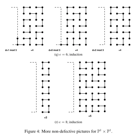
d=2 mod 3 +4 d=0 mod 3 +4 +4 d=1 mod 3 (q) e = 6; induction +2 +5 (r) e = 8; induction
Figure 4: More non-defective pictures for P1× P1.
(a) B1,1,1 (b) B2,1,1 (c) induction for B∗,1,1 (d) B2,2,1
(e) B3,2,1 (f) B4,2,1 (g) B5,2,1
B3,2,1
(h) induction for B∗,2,1
4
Secant dimensions of P
1× P
1We retain the notation of Section 3. To prove Theorem 1.1, let X = P1× P1, G =
SL2× SL2, and V = Sd(K2) ⊗ Se(K2). The polynomial map
Ψ : (t0, t1, t2) 7→ t0(x1+ t1x2)d⊗ (x1+ t2x2)e,
is dominant into the cone C over X, and M = B is the rectangular grid {0, . . . , d} × {0, . . . , e}. We may assume that d ≥ e. The building blocks of our non-defective pictures will be equivalent to {0}, {0, e1}, or {0, e1, e2}. In particular, Lemma 2.4 can be applied
directly to the barycentres of these blocks — there are no snakes and no threats.
First, if e = 2 and d is even, then (d + 1)C is known to be defective, that is, it does not fill V but is given by some determinantal equation; see [7, Example 3.2]. The argument below will show that its defect is not more than 1.
Figure 4 gives non-defective pictures for e = 1, 2, 3, 4, 5 and d ≥ e, except for e = 2 and d even. This implies, by transposing pictures, that there exist non-defective pictures for e = 6 and d = 1, 3, 4, 5. Figure 4p gives a non-defective picture for (d, e) = (6, 6). Then, using the two induction steps in Figure 4q, we find non-defective pictures for e = 6 and all d 6= 2. A similar reasoning gives non-defective pictures for e = 8 and all d 6= 2. Finally, let d ≥ e ≥ 6 be arbitrary with (d, e) 6∈ 2N × {2}. Write e + 1 = 6q + r with r ∈ {0, 2, 4, 5, 7, 9}. Then we find a non-defective picture for (d, e) by gluing q non-defective pictures for (d, 5) and, if r 6= 0, one non-defective picture for (d, r − 1) on top of each other. This proves Theorem 1.1.
5
Secant dimensions of P
1× P
1× P
1Now we turn to Theorem 1.2. Cutting to the chase, M = B is the block {0, . . . , d} × {0, . . . , e}×{0, . . . , f }. We denote the picture for this block by Bd,e,f. When convenient
we assume that d ≥ e ≥ f . First, for e = f = 1 and d even, the d + 1-st secant variety, which one would expect to fill the space, is in fact known to be defective, see [6]. The pictures below show that the defect is not more than 1.
Figure 5 gives inductive constructions for pictures for (e, f ) ∈ {(1, 1), (2, 1)} that are non-defective except for (e, f ) = (1, 1) and d even. The grey shades serve no other purpose than to distinguish between front and behind.
Rotating appropriately, this also gives non-defective pictures B1,3,1and B2,3,1;
Fig-ure 6b then gives an inductive construction of non-defective pictFig-ures Bd,3,1for d ≥ 3.
So far we have found non-defective pictures B2,4,1and B3,4,1(just rotate those B4,2,1
and B4,3,1). Figure 6c gives a non-defective picture B4,4,1. A non-defective picture B5,4,1
can be constructed from a B5,1,1and B5,2,1. Now let d ≥ 6 and write d + 1 = 4q + r with
q ≥ 0 and r ∈ {3, 4, 5, 6}. Then using q copies of B3,4,1and 1 copy of Br−1,4,1, we can
build a non-defective picture Bd,4,1; see Figure 6d for this inductive procedure.
We already have non-defective pictures B1,5,1 and B2,5,1. For d ≥ 3, write d +
1 = q ∗ 2 + r with r ∈ {2, 3}. Then a non-defective picture Bd,5,1can be constructed
from q copies of our non-defective picture B1,5,1and 1 copy of our non-defective picture
(a) B3,3,1 (b) induction for B∗,3,1 (c) B4,4,1 B3,1,1 B3,2,1 B3,4,1 (d) induction for B∗,4,1
Figure 6: Non-defective pictures for B∗,3,1and B∗,4,1.
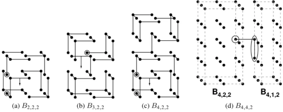
(a) B2,2,2 (b) B3,2,2 (c) B4,2,2
B4,2,2 B4,1,2
(d) B4,4,2
Figure 7: Non-defective pictures for some B∗,∗,2.
Let d ≥ e ≥ 6 and write e + 1 = q ∗ 4 + r with r ∈ {3, 4, 5, 6}. Then we can construct a non-defective picture Bd,e,1 by putting together q non-defective pictures Bd,3,1and 1
non-defective picture Bd,r−1,1. This settles all cases of the form Bd,e,1.
Figure 7a gives a picture for (d, e, f ) = (2, 2, 2), The picture is defective, but it shows that kX has the expected dimension for k = 1, . . . , 6 and defect at most 1 for k = 7. From [6] we know that 7X is, indeed, defective, so we are done. Figure 7b gives a non-defective picture B3,2,2. Similarly, Figure 7c gives a non-defective picture B4,2,2.
Now let d ≥ 5 and write d + 1 = (3 + 1)q + (r + 1) with r ∈ {1, 3, 4, 6}. Then we can construct a non-defective picture Bd,2,2from q copies of the non-defective picture B3,2,2and one non-defective picture Br,2,2. This settles Bd,2,2.
For B2,3,2and B1,3,2we have already found non-defective pictures. For d ≥ 3 write
d + 1 = 2q + (r + 1) with r ∈ {1, 2}. Then one can construct a non-defective picture Bd,3,2 from q non-defective pictures B1,3,2 and one non-defective picture Br,3,2. This
B
4,4,1B
4,4,2Figure 8: B4,4,4.
If d + 1 is even, then we can a construct non-defective picture Bd,e,2with d ≥ e ≥ 2
as follows: write e + 1 = 2q + (r + 1) with r ∈ {1, 2}, and put together q non-defective pictures Bd,1,2and one non-defective picture Bd,r,2.
Figure 7d shows how a copy of our earlier non-defective picture B2,4,2 and a
non-defective picture B1,4,2 can be put together to a non-defective picture B4,4,2. Now let
d ≥ 6 be even and write d + 1 = 4q + (r + 1) with r ∈ {2, 4}. Then one can construct a non-defective picture Bd,4,2from q copies of our non-defective picture B3,4,2and one
non-defective picture Br,4,2. This settles Bd,4,2.
Now suppose that d ≥ e ≥ 5 and f = 2. Write e + 1 = 4 ∗ q + (r + 1) with r ∈ {1, 2, 3, 4}. Then we can construct a non-defective picture Bd,e,2 from q non-defective pictures Bd,3,2and one non-defective picture Bd,r,2. This concludes the case where d ≥ e ≥ f = 2.
Consider the case where d ≥ e ≥ f = 3. This case is easy now: write, for instance, e + 1 = q ∗ 2 + (r + 1) with r ∈ {1, 2}. Then a non-defective picture Bd,e,3 can be
constructed from q non-defective pictures Bd,1,3and one non-defective picture Bd,r,3.
The above gives (by rotating) non-defective pictures Bd,e,4 for all d ≥ 1 and e ∈
bit of explanation: the upper half is the non-defective picture B4,4,1, of Figure 6c, except
that the redundant two vertices have been separated. The lower half is the non-defective picture B4,4,2 of Figure 7d. By joining the lower one of the superfluous vertices in the
upper half with the triangle in the lower half, we create a non-defective picture B4,4,4.
The newly created snake does not threaten any building block, as the picture shows, nor are the heads of this snake threatened by other snakes. Now suppose that d ≥ e ≥ 5 and write e + 1 = 4q + (r + 1) with r ∈ {1, 2, 3, 4}. Then we find a non-defective picture Bd,e,4from q non-defective pictures Bd,3,4and one non-defective picture Bd,r,4.
Finally, suppose that d ≥ e ≥ f ≥ 5, and write f + 1 = 4q + (r + 1) with r ∈ {1, 2, 3, 4}. Then a non-defective picture Bd,e,f can be assembled from q
non-defective pictures Bd,e,3and one non-defective picture Bd,e,r. This concludes the proof
of Theorem 1.3.
6
Secant dimensions of P
2× P
1For Theorem 1.3 we first deal with the defective cases: the Segre–Veronese embeddings of degree (2, even) are all defective by [7, Example 3.2]. That the embedding of degree (3, 1) is defective can be proved using a polynomial interpolation argument, used in [5] for proving defectiveness of other secant varieties: Split (3, 1) = (2, 0) + (1, 1). Now it is easy to see that given 5 general points there exist non-zero forms f1, f2 of
multi-degrees (2, 0) and (1, 1), respectively, that vanish on those points. But then the product f1f2 vanishes on those points together with all its first-order derivatives; hence the 5-th
secant variety does not fill the space. The proof below shows that its codimension is not more than 1.
For the non-defective proofs we have to solve the optimisation problems AP(B, k), where
B = {(x, y, z) ∈ Z3| x, y, z ≥ 0, x + y ≤ d, and z ≤ e}.
We shall do a double induction over the degrees e and d: First, in Subsections 6.1–6.4 we treat the cases where e is fixed to 1, 2, 3, 4, respectively, by induction over d. Then, in Subsection 6.5 we perform the induction over e. We shall always think of the x-axis as pointing towards the reader, the y-axis as pointing to the right and the z-axis as the vertical axis. The picture for (d, e) will be denoted by Td,e. We shall also use
(non-defective) pictures Ba,b,cfrom Section 5 as building blocks.
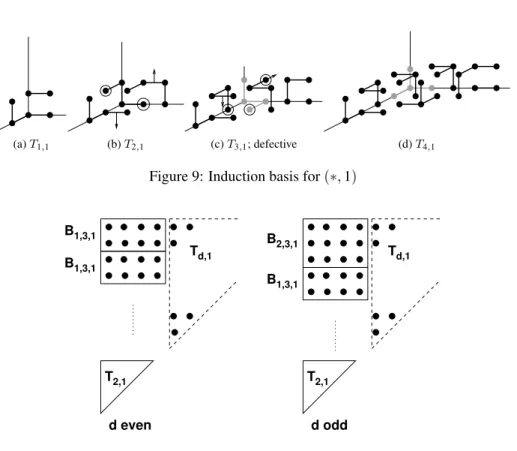
6.1 The cases where e = 1. Figures 9a–9d give pictures for (d, 1) with d = 1, . . . , 4. Now we explain how to construct a defective picture for (d + 4, 1) from a non-defective picture for (d, 1). First translate Td,1four steps in the positive x-direction, and
then proceed as follows.
(1) If d + 1 is even, d + 1 = 2l for some l, then put l copies of B1,3,1to the left of Td,1,
starting at the origin. Finally, add a copy of T2,1.
(2) If d + 1 is odd, d + 1 = 2l + 1 for some l, then put one copy of B2,3,1and l − 1 copies
of B1,3,1to the left of Td,1. Finally, add another copy of T2,1.
(a) T1,1 (b) T2,1 (c) T3,1; defective (d) T4,1
Figure 9: Induction basis for (∗, 1)
T2,1 T2,1 B1,3,1 B1,3,1 B1,3,1 B2,3,1 d even d odd Td,1 Td,1
Figure 10: Induction step for (∗, 1)
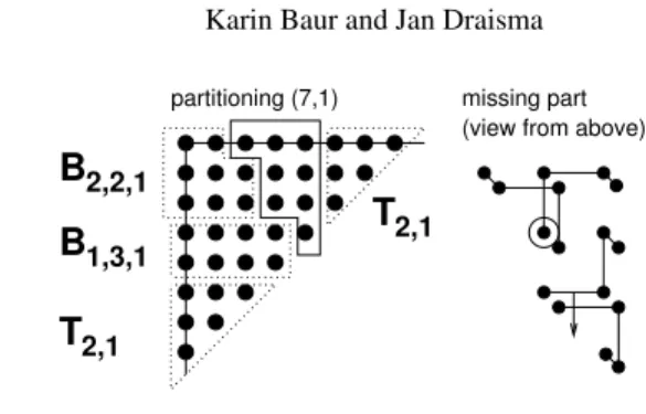
To complete the induction, since T3,1 is defective, we need a non-defective picture
for (7, 1). We can construct this from two copies of T2,1, one B1,3,1 and one B2,2,1(at
the origin) from Figure 5d. The remaining vertices are grouped together as in Figure 11 below. Note that one can separate the building blocks in this figure by successive planar cuts, so that Lemma 2.2 applies.
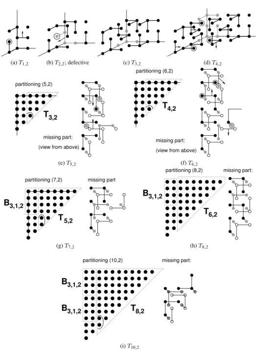
6.2 The cases where e = 2. Figures 12a–12i lay the basis for the induction over d.
Note that T6,2 is the first among the pictures whose number of vertices is divisible by 4.
To finish the induction, we need to construct a non-defective picture for (d + 8, 2) from Td,2. First of all, move Td,2eight positions to the right. Then proceed as follows:
(1) If d is odd, d = 2l + 1 for some l ≥ 0, put l pairs of B1,3,2to the right of Td,2(starting
at the origin), then two copies of B2,3,2, and finally a copy of T6,2.
(2) If d is even, d = 2l for some l > 0, put l + 1 pairs of B1,3,2starting at the origin.
Finish off with one copy of T6,2.
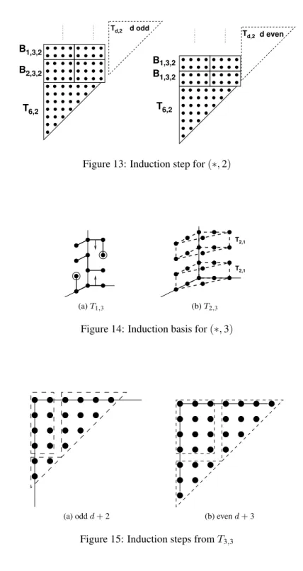
This is illustrated in Figure 13.
6.3 The cases where e = 3. Here the induction over d is easier since every Td,3has
B
2,2,1B
1,3,1T
2,1T
2,1partitioning (7,1) missing part (view from above)
Figure 11: Obtaining T7,1
(the latter just consists of two copies of T2,1). Now we show that from a non-defective
Td,3with d odd one can construct non-defective Td+2,3and Td+3,3. Write d = 2l + 1, and
proceed as follows.
(1) Move T2l+1,3 two positions to the right. Put a block B2l+1,1,3 at the origin, and
conclude with a copy of T1,3. This gives T2l+3,3.
(2) Move T2l+1,3three steps to the right. Put a block B2l+1,2,3at the origin, and conclude
with a copy of T2,3.
For d = 3 this is illustrated in Figure 15.
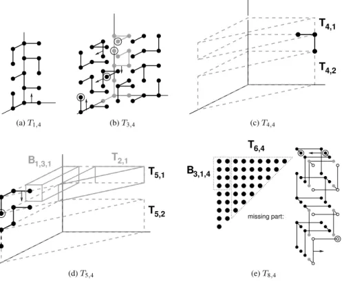
6.4 The cases where e = 4. We proceed by induction. The induction step is identical to that for e = 2, except that the blocks B1,3,2and B2,3,2have to be replaced by the blocks
B1,3,4and B2,3,4, and T6,2has to be replaced by T6,4. To lay the basis for the induction
we need pictures for d = 1, 2, 3, 4, 5, 6, 7, 8, 10, where the last one is needed since (2, 4) is defective. If (d + 1)(d + 2), which is the number of points in Td,1, is a multiple
of 4 and both Td,1 and Td,2 are non-defective, then a non-defective Td,4 is obtained by
stacking Td,1on top of Td,2. This is the case for d = 6, 7, 10. The same construction for
d = 2 leads to a defective picture T2,4, which shows that the defects are not worse than
Theorem 1.3 claims. Hence only pictures Td,4for d = 1, 3, 4, 5, 8 are needed, and these are in Figures 16a–16e.
6.5 Induction over e. From a defective picture for (d, e) we can construct a non-defective picture for (d, e + 4) by stacking a non-non-defective picture for (d, 3), whose num-ber of vertices is divisible by 4, on top of it. This settles all (d, e) except for those that are modulo (0, 4) equal to the defective (3, 1) or (2, 2). The latter are easily handled, though: stacking copies of T2,1on top of T2,2gives pictures for all (2, e) with e even that
are defective but give the correct, known, secant dimensions. So to finish our proof of Theorem 1.3 we only need the non-defective picture for (3, 5) of Figure 17.
(a) T1,2 (b) T2,2; defective (c) T3,2 (d) T4,2
partitioning (5,2)
missing part: (view from above)
T
3,2(e) T5,2
T
4,2partitioning (6,2)
missing part: (view from above)
(f) T6,2
partitioning (7,2) missing part
B
3,1,2T
5,2(g) T7,2
partitioning (8,2) missing part:
B
3,1,2T
6,2 (h) T8,2 missing part: partitioning (10,2)T
8,2B
3,1,2B
3,1,2 (i) T10,2T6,2 B1,3,2 B2,3,2 T6,2 B1,3,2 B1,3,2 Td,2 d odd Td,2 d even
Figure 13: Induction step for (∗, 2)
(a) T1,3
T2,1
T2,1
(b) T2,3
Figure 14: Induction basis for (∗, 3)
(a) odd d + 2 (b) even d + 3
(a) T1,4 (b) T3,4 T4,1 4,2 T (c) T4,4 T5,1 T5,2 B1,3,1 T2,1 (d) T5,4 missing part: B3,1,4 T6,4 (e) T8,4
Figure 16: Induction basis for (∗, 4)
7
Secant dimensions of the point-line flag variety F
In this section, X = F , G = SL3, and the highest weight λ equals mω1+ nω2 with
m, n > 0.
Remark 7.1. For the geometrically inclined reader we recall that the SL3-equivariant
embedding of F corresponding to highest weight λ is the one corresponding to the line bundle SL3/B ×BK−λ→ SL3/B = X where B is the Borel subgroup and K−λis the
one-dimensional representation of B on which the torus T ⊆ B acts with weight −λ. The global sections of this line bundle form an irreducible SL3-module of highest weight λ by
the Borel–Weil–Bott theorem. Below we shall point out a basis of this module consisting of PBW-monomials, which are in particular T -weight vectors. Unlike in the situation for Segre–Veronese embeddings, the T -weight spaces are not one-dimensional here, and we shall choose, in each weight space, PBW-monomials that are “small” in a suitable sense. We first argue that (m, n) = (1, 1) and (m, n) = (2, 2) yield defective embeddings of F . The first weight is the adjoint weight, so the cone C1,1over the image of F is just the
set of rank-one, trace-zero matrices in sl3, whose secant dimensions are well known. For
the second weight let C2,2be the image of C1,1under the map sl3 → S2(sl3), v 7→ v2.
Then C2,2 spans the SL3-submodule (of codimension 9) in S2(sl3) of highest weight
2ω1 + 2ω2, while it is contained in the quadratic Veronese embedding of sl3. Viewing
the elements of S2(sl
3) as symmetric 8 × 8-matrices, we find that C2,2 consists of rank
1 matrices, while it is not hard to prove that the module it spans contains matrices of full rank 8. Hence 7C2,2cannot fill the space.
For the non-defective proofs let α1, α2 be the simple positive roots, so that X(u) =
{β1, β2, β3} with β1 = −α1, β2 = −α1− α2 and β3 = −α2. The subscripts indicate
the order in which the PBW-monomials are computed: for r = (n1, n2, n3) we write
mr:= Xβn11X n2 β2X n3 β3vλ. Set B := {(n1, n2, n3) ∈ Z3| 0 ≤ n2≤ m, 0 ≤ n3≤ n, and 0 ≤ n1≤ m + n3− n2},
and let M be the set of all r ∈ NX(u) with m
r 6= 0. We shall not need M explicitly; it
suffices to observe that r3≤ n for all r ∈ M : indeed, if r3> n then Xβr33vλis already 0, hence so is mr. We use the following consequence of the theory of canonical bases; see
[8, Example 10, Lemma 11].
Lemma 7.2. The mb,b ∈ B, form a basis of V .
Remark 7.3. The map (n1, n2, n3) 7→ (n1, n − n3, m − n2) sends the set B, which
corresponds on the highest weight (m, n), to the set corresponding to the highest weight (n, m). Hence if we have a defective picture for one, then we also have a non-defective picture for the other. We shall use this fact occasionally.
We want to apply Lemma 2.6. First note that r, r0 ∈ RX(u)
= R3 have the same
weight if and only if r − r0 is a scalar multiple of z := (1, −1, 1). We set r < r0if and only if r − r0is a positive scalar multiple of z.
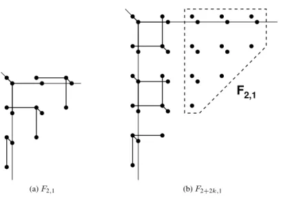
(a) F2,1
F
2,1(b) F2+2k,1
Figure 18: Pictures Feven,1.
Lemma 7.4. For all r ∈ M \ B and all b ∈ B with ξ(b) = ξ(r) we have b < r, i.e., the differenceb − r is a positive scalar multiple of z.
Proof. Suppose that b = (n1, n2, n3) ∈ B and that n3< n. Then the defining inequalities
of B show that b + z = (n1+ 1, n2− 1, n3+ 1) also lies in B. This shows that B is a
lower idealin (M, ≤), i.e., if b ∈ B and r ∈ M with r < b, then also r ∈ B. This readily
implies the lemma. 2
Proposition 7.5. AP∗(B, k) is a lower bound on dim kC for all k.
Proof. This follows immediately from Lemma 2.6 and Lemma 7.4 when we take for Z
the one-dimensional cone R≥0· z. 2
In what follows we denote the picture for (m, n) by Fm,n, and we shall assume that
m ≥ n when convenient. We first prove, by induction over m, non-defectiveness for (m, 1) and (m, 2), and then do induction over n to conclude the proof. Figure 19a for (m, n) = (1, 1) is not non-defective, reflecting that the adjoint minimal orbit — the cone over which is the cone of 3 × 3-matrices with trace 0 and rank ≤ 1 — is defective. Figure 18a, however, shows a non-defective picture F2,1, and from this picture one can
construct non-defective pictures F2+2k,1 by putting it to the right of k pictures, each of
which consists of cubes and a single corner; Figure 18b illustrates this for the step from F2,1to F2+2,1.
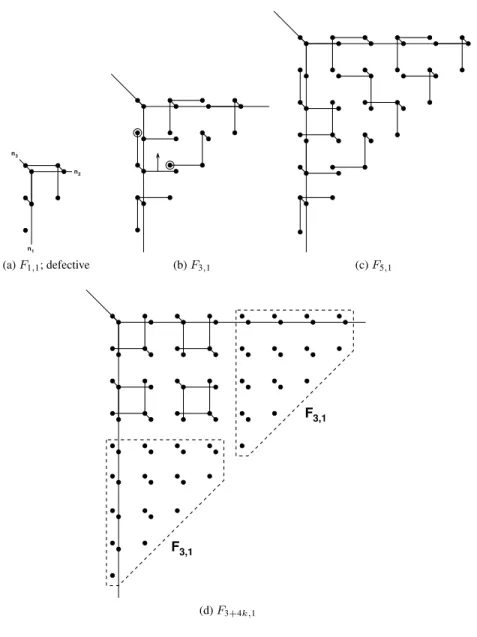
Figure 19b shows a non-defective picture for F3,1, and Figure 19c a non-defective
picture F5,1. From these we can construct non-defective pictures F3+4k,1 and F5+4k,1,
respectively, by putting them to the right of k pictures, each of which consists of a few cubes plus a non-defective picture for F3,1— Figure 19d illustrates this for the step from
n1 n3 n2 (a) F1,1; defective (b) F3,1 (c) F5,1 F3,1 F3,1 (d) F3+4k,1
(a) F2,2; defective !! (b) F3,2 (c) F4,2 (d) F5,2 B3,1,2 F4,2 (e) F6,2 F4,2 B3,2,2 (f) F7,2 B1,7,2 F7,2 F1,2 (g) Fm+8,2 Figure 20: Pictures F∗,2
F
3,1F
3,2B
2,3,1Figure 21: Construction for m or n odd.
Figure 20a is defective: it reflects the fact that the 7-th secant variety of X in the F2,2-embedding has defect 1. Figure 20b gives a non-defective picture F3,2. Note that
one non-standard cells Biis used here; this is because we want to line up the single edge
with a single vertex in the construction of F6,6. The non-standard block and the edge can
be cut of from the rest by a planar cut, so that Lemma 2.2 yields non-defectiveness of F3,2. Figure 20c gives a non-defective picture F4,2. Figures 20d, 20e, and 20f give
non-defective F5,2, F6,2, F7,2. Similarly, one can construct pictures F8,2and F10,2— which are
left out here because they take too much space. Finally, from a non-defective picture Fm,2
(with m = 1 or m ≥ 3) one can construct a non-defective picture Fm+8,2by inserting an
F7,2and a block Bm,7,2in front — Figure 20g illustrates this for m = 1. This settles the
cases where m ≥ n = 2.
Now all cases where at least one of m and n is odd can also be settled. Indeed, suppose that m, n ≥ 3 and that m is odd. Write n + 1 = 2q + (r + 1) with r ∈ {1, 2}. Then we can construct a non-defective picture Fm,nby taking our non-defective picture Fm,r
and successively stacking q non-defective pictures of two layers on top, each of which pictures with a number of vertices divisible by 4. These layers can be constructed as
(a) F4,4 F4,4 1,5,4 B (b) F6,4 F3,3 F3,2 B3,2,6 B 3,3,2 F2,6 (c) F6,6
follows: the i-th layer consists of a block Br+2i−2,m,1(lying against the (n2, n3)-plane)
and a non-defective picture Fm,1. As m is odd, each of these two blocks has a number of
vertices divisible by 4. This construction is illustrated for m = 3 and n = 4 in Figure 21, where one extra layer is put on top of the “ground layer”.
Only the cases remain where m and n are both even. We first argue that we can now reduce the discussion to a finite problem: if m ≥ 7 and n ≥ 2, then we can compose a non-defective picture Fm,n from one non-defective picture F7,n (which exists by the
above), one non-defective block B7,m−8,n(both of these have numbers of vertices
divis-ible by 4), and one non-defective picture Fm−8,n— if such a picture exists. Hence we may assume that m < 7. Similarly, by using Remark 7.3 we may assume that n < 7. Using that m, n are even, and that m, n > 2 (which we have already dealt with), we find that only (4, 4), (4, 6) (or (6, 4)), and (6, 6) need to be settled — as done in Figures 22a– 22c. The picture F6,6is built from a block B3,2,6, one F2,6obtained from F6,2, and one
F3,6; the latter picture, in turn, can be constructed as outlined above, except that, in order
to line up the single edge in F3,6and the single vertex in F2,6, the order of the building
blocks for F3,6is altered: F3,2comes on top, next to a block B3,3,2, and under these a
copy of F3,3. This is where we use that in F3,2the remaining two vertices form an edge in
a convenient position, this explains the use of the non-standard building block for F3,2. It
is easy to see that the left-hand side of the picture, together with the single edge of F3,2in
the right-hand side, can be separated from the rest with a plane, so that Lemma 2.2 yields non-defectiveness. This concludes the proof of Theorem 1.4.
References
[1] J. Alexander, A. Hirschowitz, Polynomial interpolation in several variables. J. Algebraic Geom.4 (1995), 201–222.MR1311347 (96f:14065) Zbl 0829.14002
[2] A. Borel, Linear algebraic groups. Springer 1991.MR1102012 (92d:20001) Zbl 0726.20030
[3] M. C. Brambilla, G. Ottaviani, On the Alexander-Hirschowitz theorem. J. Pure Appl. Algebra 212 (2008), 1229–1251.MR2387598 (2008m:14104) Zbl 1139.14007
[4] S. Brannetti, Degenerazioni di Variet`a Toriche e Interpolazione Polinomiale. PhD thesis, Uni-versit`a di Roma “Tor Vergata”, 2007.
[5] M. V. Catalisano, A. V. Geramita, A. Gimigliano, Higher secant varieties of Segre-Veronese varieties. In: Projective varieties with unexpected properties, 81–107, de Gruyter 2005.
MR2202248 (2007k:14109a) Zbl 1102.14037
[6] M. V. Catalisano, A. V. Geramita, A. Gimigliano, Segre–Veronese embeddings of P1× P1× P1 and their secant varieties. Collect. Math. 58 (2007), 1–24. MR2310544 (2008f:14069)
Zbl 1122.14037
[7] M. V. Catalisano, A. V. Geramita, A. Gimigliano, On the ideals of secant varieties to certain rational varieties. J. Algebra 319 (2008), 1913–1931.MR2392585 (2009g:14068) Zbl 1142.14035
[8] W. A. de Graaf, Five constructions of representations of quantum groups. Note Mat. 22 (2003/04), 27–48.MR2106571 (2005i:17018) Zbl 1097.17013
[9] M. Develin, Tropical secant varieties of linear spaces. Discrete Comput. Geom. 35 (2006), 117–129.MR2183492 (2006g:52024) Zbl 1095.52006
[10] J. Draisma, A tropical approach to secant dimensions. J. Pure Appl. Algebra 212 (2008), 349– 363.MR2357337 (2008j:14102) Zbl 1126.14059
[11] J. Harris, Algebraic geometry. Springer 1992.MR1182558 (93j:14001) Zbl 0779.14001
[12] J. E. Humphreys, Introduction to Lie algebras and representation theory. Springer 1972.
MR0323842 (48 #2197) Zbl 0254.17004
[13] B. Sturmfels, S. Sullivant, Combinatorial secant varieties. Pure Appl. Math. Q. 2 (2006), 867– 891.MR2252121 (2007h:14082) Zbl 1107.14045
Received 19 July, 2007; revised 9 February, 2009
K. Baur, ETH Z¨urich, Departement Mathematik, R¨amistrasse 101, 8092 Z¨urich, Schweiz Email: [email protected]
J. Draisma, Department of Mathematics and Computer Science, Technische Universiteit Eindhoven, P.O. Box 513, 5600 MB Eindhoven, The Netherlands, and Centrum voor Wiskunde en Infor-matica, Amsterdam, The Netherlands