Clustered Naive Bayes

Clustered Naive Bayes

by

Daniel Murphy Roy

Submitted to the Department of Electrical Engineering and Computer Science

in partial fulfillment of the requirements for the degree of

Masters of Engineering in Electrical Engineering and Computer Science

at the

MASSACHUSETTS INSTITUTE OF TECHNOLOGY

May 2006

@ Daniel Murphy Roy, MMVI. All rights reserved.

The author

paper

hereby grants to MIT permission to reproduce and distribute publicly

and electronic copies of this thesis document in whole or in part.

A uth or ...

...

Department of Electrical IENgineering and Computer Science

May 25, 2006

Certified by ...

Professor of Electrical

Accepted by ...

Chairman, Depar

Leslie Pack Kaelbling

Engineering and Computer Science

Thesis Supervisor

... ...

Arthur C. Smith

tment Committee on Graduate Students

MASSACHUSETTS INS1TIUTE

OF TECHNOLOGY _BARKER

Clustered Naive Bayes

Daniel Murphy Roy

Submitted to the Department of Electrical Engineering and Computer Science on May 25, 2006, in partial fulfillment of the

requirements for the degree of

Masters of Engineering in Electrical Engineering and Computer Science

Abstract

Humans effortlessly use experience from related tasks to improve their performance at novel tasks. In machine learning, we are often confronted with data from "related" tasks and asked to make predictions for a new task. How can we use the related data to make the best prediction possible? In this thesis, I present the Clustered Naive Bayes classifier,

a hierarchical extension of the classic Naive Bayes classifier that ties several distinct Naive Bayes classifiers by placing a Dirichlet Process prior over their parameters. A priori, the model assumes that there exists a partitioning of the data sets such that, within each subset, the data sets are identically distributed. I evaluate the resulting model in a meeting domain, developing a system that automatically responds to meeting requests, partially taking on the responsibilities of a human office assistant. The system decides, based on a learned model of the user's behavior, whether to accept or reject the request on his or her behalf. The extended model outperforms the standard Naive Bayes model by using data from other users to influence its predictions.

Thesis Supervisor: Leslie Pack Kaelbling

Acknowledgments

All of my achievements to date were possible only with the support provided to me by a

handful of individuals. Most immediately, this work would not have been possible without my thesis advisor, Leslie Kaelbling, who took me on as a student last year and has, since then, given me full reign to chase my interests. Leslie has an amazing ability to see through the clutter of my reasoning and extract the essence; the various drafts of this thesis improved

by leaps and bounds each time Leslie gave me comments.

I would also like to thank Martin Rinard, who was the first professor at MIT to invite

me to work with him. Martin encouraged me to apply to the PhD program and then championed my application. I learned many valuable lessons from Martin, most of them late at night, working on drafts of papers due the next day. Every so often, I hear Martin in the back of my head, exclaiming, "Be brilliant!" Of course!

I would like to thank Joann P. DiGennaro, Maite Ballestero and the Center for

Excel-lence in Education for inviting me to participate in the Research Science Institute in 1998. They accepted my unorthodox application, taking a risk with a student with much less exposure to academic research than his peers. I flourished under their guidance and owe them an enormous debt of gratitude. I would also like to thank my teachers at Viewpoint School who pushed me to reach my full potential and more than prepared me for MIT.

I am incredibly grateful for the sacrifices my parents made in sending me to the best schools possible. I would like to thank my father for buying my first computer, my mother for buying my first cello, and my two brothers, Kenny and Matt, for being my closest friends growing up. Finally, I would like to thank Juliet Wagner, who five years ago changed my life with a single glance.

Contents

1 Introduction 6

2 Models 14

2.1 Naive Bayes models . . . . 15

2.2 No-Sharing Baseline Model . . . . 17

2.3 Complete-Sharing Model. . . . . 18

2.4 Prototype Model . . . . 20

2.5 The Clustered Naive Bayes Model . . . . 23

3 The Meeting Task and Metrics 27 3.1 Meeting Task Definition . . . . 28

3.1.1 Meeting Representation . . . . 29

3.1.2 Dataset specification . . . . 29

3.2 Evaluating probabilistic models on data . . . . 31

3.2.1 Loss Functions on Label Assignments . . . . 32

3.2.2 Loss Functions on Probability Assignments . . . . 35

4 Results 38 4.1 No-Sharing Model . . . . 38

4.2 Complete-Sharing Model. . . . . 41

4.3 Clustered Naive Bayes Model . . . . 47

A Implementing Inference

A.1 Posterior Distributions: Derivations and Samplers . . . .

A.1.1 No-Sharing Model . . . .

A.1.2 Complete-Sharing Model . . . .

A.1.3 Clustered Naive Bayes . . . .

A.2 Calculating Evidence and Conditional Evidence . . . .

A .2.1 Evidence . . . .

A.2.2 Conditional Evidence . . . .

A.2.3 Implementing AIS to compute the conditional evidence

B Features 5 55 57 57 60 . . . . 63 . . . . 64 . . . . 64 . . . . 65 . . . . 67 70

I

Chapter 1

Introduction

In machine learning, we are often confronted with multiple, related datasets and asked to make predictions. For example, in spam filtering, a typical dataset consists of thousands of labeled emails belonging to a collection of users. In this sense, we have multiple data sets-one for each user. Should we combine the datasets and ignore the prior knowledge that different users labeled each email? If we combine the data from a group of users who roughly agree on the definition of spam, we will have increased the available training data from which to make predictions. However, if the preferences within a population of users are heterogeneous, then we should expect that simply collapsing the data into an undifferentiated collection will make our predictions worse. Can we take advantage of all the data to improve prediction accuracy even if not all the data is relevant?

The process of using data from unrelated or partially related tasks is known as transfer

learning or multi-task learning and has a growing literature (Thrun, 1996; Baxter, 2000;

Guestrin et al., 2003; Xue et al., 2005; Teh et al., 2006). While humans effortlessly use experience from related tasks to improve their performance at novel tasks, machines must be given precise instructions on how to make such connections. In this thesis, I introduce such a set of instructions, based on the statistical assumption that there exists some partitioning of the data sets into groups such that each group is identically distributed. Because I have made no representational commitments, the assumptions are general but weak. Ultimately, any such model of sharing must be evaluated on real data to test its worth, and, to that end,

responds to meeting requests, partially taking on the responsibilities of a human office assistant. The system decides, based on a learned model of the user's behavior, whether to accept or reject the request on his or her behalf. The model with sharing outperforms its non-sharing counterpart by using data from other users to influence its predictions.

In the machine learning community, prediction is typically characterized as a

classifi-cation problem. In binary classificlassifi-cation, our goal is to learn to predict the outputs of a

(possibly non-deterministic) function

f

the missing label Yn+1. However, before a prediction is decided upon, we must first formally specify our preferences with respect to prediction error. This is accomplished by defining a loss function, L(y, y'), which specifies the penalty associated with predicting the label y' when the true label is y. For example,

L(yy') = y=y11

is referred to as 0-1 loss. Inspecting Equation (1.1), we see that the classifier is penalized if it predicts the wrong label and is not penalized if it predicts the correct label. It follows from this definition that the optimal decision is to choose the most likely label. In a spam filtering setting, however, the 0-1 loss is inappropriate; we would prefer to allow the odd spam email through the filter if it lowered the chance that an authentic email would be discarded. Such loss functions are called asymmetric because they assign different loss depending on whether the true label is zero or one.

In the standard classification setting, the example input/output pairs are assumed to be independent and identically distributed (i.i.d.) samples from some unknown probabil-ity distribution, P(X, Y). In fact, if we know P(X, Y), then, given any unlabeled input Xn+1 = x and any loss function L(y, y'), we can determine the prediction that minimizes the expected loss by choosing the label

yopt = arg min E[L(Y, y')IX = x]. (1.2)

L(y, y')

?(XY)

P(X,Y|D)

argmin

Yn+1

- Inference _{E [L(Y, y')ID, X = X.+]}

D=(Xi,

Y)

X

Figure 1-1: Given a probabilistic model,

P(X,

loss function L(y, y') and an unlabeled input Xn+1, we can immediately choose the label

that minimizes the expected loss.

From this perspective, if we can build a probabilistic model

P(X,

close to the true distribution P(X, Y), then we can make predictions for a range of loss functions (see Figure 1-1). For any particular loss function, empirical assessments of loss can be used to discriminate between probabilistic models (Vapnik, 1995). However, in order to handle a range of loss functions, we should not optimize with respect to any one particular loss function. While we could handle over-specialization heuristically by using several representative loss functions, we will instead directly evaluate the probability assignments that each model makes.

Recall that the monotonicity of the log function implies that maximizing the likelihood is identical to maximizing the log-likelihood. Using Gibbs' inequality, we can interpret the effect of seeking models that maximize the expected log-likelihood. Given two distribution p(.) and q(.), Gibbs' inequality states that,

Ep[logp(x)] ;> Ep[logq(x)],

(1.3)

with equality only if p = q almost everywhere. Consider the task of choosing a distribution q to model data generated by an unknown probability distribution p. By Gibbs inequality, the distribution q that maximizes the expected log-likelihood of the data,

Ep[log q(x)],

(1.4)

is the only loss function on distributions such that minimizing the expected loss leads invariably to true beliefs (Merhav, 1998).1

The difference between the expected log-likelihood under the true model p and any approximate model q is

Ep[logp(x)] - Ep[logq(x)] = E,[log ] = D(pflq), (1.5)

q(x)

where D(p| q) is known as the relative entropy of p with respect to q.2 Therefore, choosing the model that maximizes the expected log-likelihood is equivalent to choosing the model that is closest in relative entropy to the true distribution. Given any finite dataset, we can produce empirical estimates of these expectations and use them to choose between models and make predictions.3

Assuming that we have decided to model our data probabilistically, how do we take advantage of related data sets? Consider the case where the datasets are each associated with a user performing a task that we intend to learn to predict. In order to leverage other users' data, we must formally define how users are related. However, while we may know several types of relationships that could exist, unless we know the intended users person-ally, we cannot know which relationships will actually exist between users in an arbitrary population. Therefore, the set of encoded relationships should include those relationships that we expect to exist in real data (so they can be found) and those that can be used to improve prediction performance (so they are useful). With real data from a group of users, we first identify which of these relationships actually hold and then take advantage of them. For example, consider the prior belief that people who receive similar email are more likely to agree on the definition of spam. Given unlabeled emails from a user, we might benefit

by grouping that user with other users whose mail is similar. On the other hand, while we

may be able to discover that two users share the same birthday, this information is unlikely to aid in learning their spam preferences.

'Technically the log-loss is the only local proper loss function, where local implies that the loss function

L(q, a) only relies on the value of the distribution q at the value a and proper implies that it leads to Bayesian beliefs. The log-loss is known as the self-information loss in the information theory literature (Barron, 1998).

2_{This quantity is also known as the Kullback-Leibler (or, KL) divergence. Note that, while relative}

entropy is non-negative and zero if and only if q = p, it is not symmetric and therefore not a distance metric.

(a) User 1 User 2 User 3 User 4 User 5 User 6

U

U.E

(b)

User I

User 2

User 3

User 4

User 5

User 6

(c)

User 1

User 2

User 3

User 4 N User 5

Ue

Classifier E User Data Set

Figure 1-2: Transfer Learning Strategies: When faced with multiple datasets (six here, but in general n) over the same input space, we can extend a model that describes a single data set to one that describes the collection of datasets by constraining the parameters of each model. (a) If a model is applied to each dataset and no constraints are placed on the parameterizations of these models, then no transfer will be achieved. (b) Alternatively, if each of the models is constrained to have the same parameterization, it is as if we trained a single model on the entire dataset. Implicitly, we have assumed that all of the data sets are identically distributed. When this assumption is violated, we can expect prediction to suffer. (c) As a compromise, assume there exists a partitioning (coloring) of the datasets into groups such that the groups are identically distributed.

When faced with a classification task on a single data set, well-studied techniques abound (Boser et al., 1992; Herbrich et al., 2001; Lafferty et al., 2001). A popular classifier that works well in practice, despite its simplicity, is the Naive Bayes classifier (Maron, 1961) (which was casually introduced over 40 years ago). However, the Naive Bayes classifier cannot directly integrate multiple related datasets into its predictions. If we train a separate classifier on each data set then, of course, it follows that the other data sets will have no effect on predictive performance (see Figure 1-2(a)). One possible way of integrating related datasets is to combine them into a single, large data set (see Figure 1-2(b)). However, just as in the spain example, grouping the data and training a single Naive Bayes classifier will work only if users behave similarly.

Consider the following compromise between these two extreme forms of sharing. Instead of assuming that every dataset is identically distributed, we will assume that some grouping of the users exists such that the datasets within each group are identically distributed (see Figure 1-2(c)). Given a partitioning, we can then train a classifier on each group. To handle uncertainty in the number of groups and their membership, I define a generative process for datasets, such that they the datasets tend to cluster into identically distributed groups. At the heart of this process is a non-parametric prior known as the Dirichlet Process. This prior ties the parameters of separate Naive Bayes models that model each dataset. Because samples from the Dirichlet Process are discrete with probability one, and therefore, exhibit clustering, the model parameterizations also cluster, resulting in identically distributed groups of data sets. This model extends the applicability of the Naive Bayes classifier to the domain of multiple, (possibly) related data sets defined over the same input space. I call the resulting classifier the Clustered Naive Bayes classifier. Bayesian inference under this model simultaneously considers all possible groupings of the data, weighing the predictive contributions of each grouping by its posterior probability.

There have been a wide variety of approaches to the problem of transfer learning. Some of the earliest work focused on sequential transfer in neural networks, using weights from networks trained on related data to bias the learning of networks on novel tasks (Pratt,

1993; Caruana, 1997). Other work has focused on learning multiple tasks simultaneously.

to achieve transfer and then extends this approach to decision-tree induction and k-nearest neighbors. More recently, these ideas have been applied to modern supervised learning algorithms, like support vector machines (Wu and Dietterich, 2004). Unfortunately, it is very difficult to interpret these ad-hoc techniques; it is unclear whether the type of sharing they embody is justified or relevant. In contrast, the probabilistic model at the heart of the Clustered Naive Bayes classifier explicitly defines the type of sharing it models.

I have taken a Bayesian approach to modelling, and therefore probabilities should be interpreted as representing degrees of belief (Cox, 1946; Halpern, 1999; Arnborg and Sjdin, 2000). This thesis is related to a large body of transfer learning research conducted in the hierarchical Bayesian framework, in which common prior distributions are used to tie together model components across multiple datasets. My work is a direct continuation of work started by Zvika Marx and Michael Rosenstein on the CALO DARPA project. Marx and Rosenstein formulated the meeting acceptance task, chose relevant features, collected real-world data sets and built two distinct models that both achieved transfer. In the first model, Marx et al. (2005) biased the learning of a logistic regression model by using a prior over weights whose mean and variance matched the empirical mean and variance of the weights learned on related tasks. Rosenstein et al. (2005) constructed a hierarchical Bayesian model where each tasks was associated with a separate naive Bayes classifier. Transfer was achieved by first assuming that the parameters were drawn from a common distribution and then performing approximate Bayesian inference. The most serious problem with this model is that the chosen prior distribution is not flexible enough to handle more than one group of related tasks. In particular, if there exists two sufficiently different groups of tasks, then no transfer will occur. I describe their prior distribution in Section 2.4. This thesis improves their model by replacing the common distribution with a Dirichlet Process prior. It is possible to loosely interpret the resulting Clustered Naive Bayes model as grouping tasks based on a marginal likelihood metric. From this viewpoint, this work is related to transfer-learning research which aims to first determine which tasks are relevant before

attempting transfer (Thrun and O'Sullivan, 1996).

Ferguson (1973) was the first to study the Dirichlet Process and show that it can, simply speaking, model any other distribution arbitrarily closely. With the advent of faster

com-puters, large-scale inference under the Dirichlet Process has become possible, resulting in a rush of research applying this tool to a wide range of problems including document mod-elling (Blei et al., 2004), gene discovery (Dahl, 2003), and scene understanding (Sudderth et al., 2005). Teh et al. (2006) introduced the Hierarchical Dirichlet Process, achieving transfer learning in document modelling across multiple corpora. The work closest in spirit to this thesis was presented recently by Xue et al. (2005). They achieved transfer learning between multiple datasets by tying the parameters of logistic regression models together using the Dirichlet Process and deriving a variational method for performing inference. In the same way, the Clustered Naive Bayes model I introduce uses a Dirichlet Process prior to tie the parameters of several Naive Bayes models together to achieve transfer. There are several important differences: First, the logistic regression model is discriminative, meaning that it does not model the distribution of the inputs. Instead, it only models the condi-tional distribution of the outputs conditioned on the inputs. As a result, it cannot take advantage of unlabeled data. In the Clustered Naive Bayes model, the datasets are clus-tered with respect to a generative model which defines a probability distribution over both the inputs and outputs. Therefore, the Clustered Naive Bayes model is semi-supervised: it can take advantage of unlabeled data points. Implicit in this choice is the assumption that similar feature distributions are associated with similar predictive distributions. Whether this assumption is valid must be judged for each task; for the meeting acceptance task, the generative model of sharing seems appropriate and leads to improved results.

This thesis is in five parts. In Chapter 2, I formally define the Clustered Naive Bayes model as well as two baseline models against which the clustered variant will be compared. In Chapter 3, I define the meeting acceptance task and justify the metrics I will use to evaluate the Clustered Naive Bayes model's performance. In Chapter 4, I present the results for the meeting acceptance task. In Chapter 5, I conclude with a discussion of the results and ideas for future work. Finally, for my most ardent readers, I present the technical aspects of performing inference in each of the models in Appendix A.

Chapter 2

Models

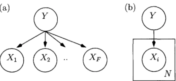
In this thesis we are concerned with classification settings where the inputs and output labels are drawn from finite sets. In particular, the inputs are composed of F features, each taking values from finite sets. Over such input spaces, the standard Naive Bayes classifier normally takes the form of a product of multinomial distributions. In this chapter I introduce the Clustered Naive Bayes model in detail, as well as two additional models which will function as baselines for comparison in the meeting acceptance task.

Let the tuple (X1, X2,..., XF) represent F features comprising an input X, where each Xi takes values from a finite set Vi. We write (X, Y) to denote a labelled set of features, where Y E L is a label. We will make an assumption of exchangeability; any

permutation of the data has the same probability. This is a common assumption in the classification setting, that states that it is the value of the inputs and outputs that determine the probability assignment and not their order. Consider U data sets, each composed of

N feature/label pairs. Simply speaking, each data set is defined over the same input

space. It should be stressed, however, that, while each dataset is assumed to be identically distributed, we do not assume that the collection of datasets are identically distributed. We will associate each data set with a particular user. Therefore, we will write D",j = (X, Y)i

and D, = (Ds,, D,,2, ... , DU,NU) to indicate the N, labelled features associated with the

u-th user. Then D is the entire collection of data across all users, and Duj = (Xu,j, Yu,) is the j-th data point for the u-th user.

(a)

(b)

Y

y

N

Figure 2-1: (a) A graphical model representing that the features X are conditionally inde-pendent given the label, Y. (b) We can represent the replication of conditional independence across many variables by using plates.

2.1

Naive Bayes models

Under the Naive Bayes assumption, the marginal distribution for j-th labelled input for the

u-th user is

F

P(Du,j) = P(Xu,,Y = P(Yu,,) H P(Xu,j,fIYu,j). (2.1) f=1

This marginal distribution is depicted graphically in Figure 2-1. Recall that each label and feature is drawn from a finite set. Therefore, the conditional distribution, P(Xu,j,fIYU,j), associated with the feature/label pair y/f is completely determined by the collection of probabilities 0u,y,f {Ou,y,f,x : x E Vf}, where

9_{uy,f,x L Pr {Xu,f = x1Y = y}. (2.2)}

To define a distribution, the probabilities for each value of the feature Xf must sum to one. Specifically, EZXEVf Ou,y,f,x = 1. Therefore, every feature-label pair is associated with

a distribution. We write 6 to denote the set of all conditional probability distributions that parameterize the model. Similarly, the marginal P(Yu) is completely determined by the probabilities Ou O{,y : y E L}, where

Again, Eycc Ou,y = 1. We will let 0 denote the collection of marginal probability distri-butions that parameterize the model. Note that each dataset is parameterized separately and, therefore, we have so far not constrained the distributions in any way. We can now write the general form of the Naive Bayes model of the data:

U

P(DO, 4) =7 P(DuI|O, OU) (2.4)

u=1

U Nu

1P1

u=1 n=1

U N, F

=

1

17P(Y,n1Ou,y)

Jj

u=1 n=1 f=1

U F

mu~y ou,y,f, u=1 yEL f=1 xEVf

where me,, is the number of data points labeled y E C in the data set associated with the

u-th user and nu,,,f,x is the number of instances in the u-th dataset where feature

f

into a product of terms, one for each dataset, reflecting that the datasets are independent conditioned on the parameterization. Equation (2.5) makes use of the exchangeability assumption; specifically, the label/feature pairs are independent of one another given the parameterization. In Equation (2.6), we have made use of the Naive Bayes assumption. Finally, in (2.7), we have used the fact that the distributions are multinomials.

To maximize P(D 6, 0) with respect to 6,

4,

OUY = MU'y (2.8) and 6 u,y,f, = uyfx (2.9) Zfx YxCVf lu,,y,f,x

Because each dataset is parameterized separately, it is no surprise that the maximum like-lihood parameterization for each data set depends only on the data in that data set. In

order to induce sharing, it is clear that we must somehow constrain the parameterization across users. In the Bayesian setting, the prior distribution P(9, 0) can be used to enforce such constraints. Given a prior, the resulting joint distribution is

P(D) = P(D1,

4)

4).

Each of the models introduced in this chapter are completely specified by particular prior distributions over the parameterization of the Naive Bayes model. As we will see, different priors result in different types of sharing.

2.2

No-Sharing Baseline Model

We have already seen that a ML parameterization of the Naive Bayes model ignores related data sets. In the Bayesian setting, any prior over the entire set of parameters that factors into distributions for each user's parameters will result in no sharing. In particular,

U

P(O, 0) =

17

u=1

is equivalent to the statement that the parameters for each user are independent of the parameters for other users. Under this assumption of independence, training the entire collection of models is identical to training each model separately on its own dataset. We therefore call this model the no-sharing model.

Having specified that the prior factors into parameter distributions for each user, we must specify the actual parameter distributions for each user. A reasonable (and tractable) class of distributions over multinomial parameters are the Dirichlet distributions which are conjugate to the multinomials. Therefore, the distribution over qu, which takes values in the LC-simplex, is

P(4U) = 42" . (2.12)

Similarly, the distribution over 0uyf, which takes values in Vf f-simplex, is

F(Zxevf

17

1uyfxl

P(Of) = EV (uyfx) 1 uyfx (2.13)

rlx~fr(3uy~~xXEVf

We can write the resulting model compactly as a generative process:1

OU ~ Dirichlet({a,y : y E L}) (2.14)

Yu, I Ou ~ Discrete(ou) (2.15)

Ou,u,f ~ Dirichlet({#u,,,j,x : x E Vf} (2.16)

X f I Yun, {Ou,y,f : Vy E Y} ~ Discrete(6u,(yfl),f) (2.17)

The No-Sharing model will function as a baseline against which we can compare alternative models that induce sharing.

2.3

Complete-Sharing Model

The Complete-Sharing model groups all the users' data together, learning a single model. We can express this constraint via a prior P(O, 0) by assigning zero probability if 9

u,y,f

$

Gu',,f for any u, u' (and similarly for Ou,y). This forces the users to share the same

param-eterization. It is instructive to compare the graphical models for the baseline No-Sharing model (Figure 2-2) and the Complete-Sharing model (Figures 2-3). As in the No-Sharing model, each parameter will be drawn independently from a Dirichlet distribution. However, while each user had its own set of parameters in the No-Sharing model, all users share the same parameters in the Complete-Sharing model. Therefore, the prior probability of the complete parameterization is

F

P(6, 0) = P(#)

]J

JJ

P(OV),

(2.18)

f=1 yEL

'The ~ symbol denotes that the variable to the left is distributed according to the distribution specified on the right. It should be noted that the Dirichlet distribution requires an ordered set of parameters while the definitions we specify provide an unordered set. To solve this, we define an arbitrary ordering of the elements of L and Vf. We can then consider the elements of these sets as index variables when necessary.

Figure 2-2: No-Sharing Graphical Model: Each ization. X~if

X 5f

Nu

U

model for each user has its own

parameter-yf 12fF

Figure 2-3: Graphical Model for Complete-Sharing model - The prior distribution over parameters constrains all users to have the same parameters.

Ybj

F

Y

E

where

F(Zyc

y)

H~~F~cy)

Again, we can represent the model compactly by specifying the generative process (c.f. (2.14)):

0 ~ Dirichlet({a., y E G}) (2.21)

Y,,I 1 ~ Discrete() (2.22)

6_{y,f ~ Dirichlet({y,f,x : x E Vf}) (2.23)}

XUn,f | Y,n, {6yj : Vy E Y} - Discrete(6(yud),f) (2.24)

While the baseline model totally ignores other datasets when fitting its parameters, this model tries to find a single parameterization that fits all the data well. If the data are unrelated, then the resulting parameterization may describe none of individual data sets accurately. In some settings, this model of sharing is appropriate. For example, for a group of individuals who agree what constitutes spam, pooling their data would likely improve the performance of the resulting classifier. However, in situations where we do not know a priori whether the data sets are related, we need a more sophisticated model of sharing.

2.4

Prototype Model

Instead of assuming that every dataset is distributed identically, we can relax this assump-tion by assuming that there exists a prototypical distribuassump-tion and that each data set is generated by a distribution that is a noisy copy of this prototype distribution. To model this idea, we might assume that every user's parameterization is drawn from a common unimodal parameter distribution shared between all users. Consider the following noise

Xuj

F

Nu

IF

U

-(9F

Figure 2-4: Prototype Model

model: For all features

f

Oy,f = {Oy,f,x

: x

Vf

},

and a strength parameter K,f > 0. Then, each parameter 9

u,,f is drawn according to a Dirichlet distribution with parameters Oy,f,x * Kyf. I will refer to this distribution over

the simplex as the noisy Dirichlet. As Kyf grows, the noisy Dirichlet density assigns most of its mass to a ball around the prototype #yj. Figure 2-5 depicts some samples from this noise model.2 One question is whether to share the parameterization for the marginal distribution, <$. Because we are most interested in transferring knowledge about the relationship between the features and the label, I have decided not to share the marginal.

2

An alternative distribution over the simplex that has a larger literature is the logistic normal distribution (Aitchison, 1982). The noisy Dirichlet has reasonable properties when K is large. However, for K < 1, the

K.10 0. 105 -02 --01 0 0!2 04 0,6 09 1 K.O.60 0" 0.. 0 0 0 0.2 0.4 DA6 0.0 1 P1 09 -O's 0.7 0.6 0 5 02 - 0 0 0 .02 4 0 9 K00 0 0 0.1 00 0.2 04 0 6 1

Figure 2-5: Noise Model Samples: The following diagrams each contain 1000 samples from the noisy Dirichlet distribution over the 3-simplex with prototype parameter 9 =

{

and strength parameter K={100, 10, 3,0.5, 0.1, 0.01}. When the value of K drops below the point at which KG has components less than 1 (in this diagram, K = 3), the distribution

becomes multimodal, with most of its mass around the extreme points.

We can write the corresponding model as a generative process

Uj, Dirichlet({3vfx : x E

Vf})

I

E

If the parameterizations of each of the data sets are nearly identical, then a fitted unimodal noise model will be able to predict parameter values for users when there is insufficient data. However, this model of sharing is brittle: Consider two groups of data sets where each group is identically distributed, but the parameterizations of the two groups are very different. Presented with this dataset, the strength parameter K will be forced to zero in order to model the two different parameterizations. As a result, no sharing

04 03 00 07 - C 06-02 0 01 0 12 0. p 0 Km.001 0.E 02 0. 0. 0 02 0.4 08 08 1 P1 (2.29) (2.30) (2.31)

Yuj 6 zyf

F

|

F

XujfN

Nu

_U

_(b)

_-(

Figure 2-6: (a) The parameters of the Clustered Naive Bayes model are drawn from a Dirichlet Process. (b) In Chinese Restaurant Process representation, each user u is associ-ated with a "table" zu, which indexes an infinite vector of parameters drawn i.i.d. from the base distribution.

will occur. Because the unimodal nature of the prior seems to be the root cause of this brittleness, a natural step is to consider multimodal prior distributions.

2.5

The Clustered Naive Bayes Model

A more plausible assumption about a group of related data sets is that some partition exists where each subset is identically distributed. We can model this idea by making the prior distribution over the parameters a mixture model. Consider a partitioning of a collection of datasets into groups. Each group will be associated with a particular parameterization of a Naive Bayes model. Immediately, several modelling questions arise. First and foremost, how many groups are there? It seems reasonable that, as we consider additional data sets, we should expect the number of groups to grow. Therefore, it would be inappropriate to choose a prior distribution over the number of groups that was independent of the number of datasets. A stochastic process that has been used successfully in many recent papers to model exactly this type of intuition is the Dirichlet Process. In order to describe this

process, I will first describe a related stochastic process, the Chinese Restaurant Process. The Chinese Restaurant Process (or CRP) is a stochastic process that induces distribu-tions over partidistribu-tions of objects (Aldous, 1985). The following metaphor was used to describe the process: Imagine a restaurant with an infinite number of indistinguishable tables. The first customer sits at an arbitrary empty table. Subsequent customers sit at an occupied table with probability proportional to the number of customers already seated at that table and sit at an arbitrary, new table with probability proportional to a parameter a > 0 (see

Figure 2.5). The resulting seating chart partitions the customers. It can be shown that, in expectation, the number of occupied tables after n customers is E(log n) (Navarro et al.,

2006; Antoniak, 1974).

To connect the CRP with the Dirichlet Process, consider this simple extension. Imagine that when a new user enters the restaurant and sits at a new table, they draw a complete parameterization of their Naive Bayes model from some base distribution. This parameter-ization is then associated with their table. If a user sits at an occupied table, they adopt the parameterization already associated with the table. Therefore, everyone at the same

table uses the same rules for predicting.

This generative process is known as the Dirichlet Process Mixture Model and has been used very successfully to model latent groups. The Dirichlet process has two parameters, a mixing parameter a, which corresponds to the same parameter of the CRP, and a base dis-tribution, from which the parameters are drawn at each new table. It is important to specify that we draw a complete parameterization of all the feature distributions, OV,f, at each ta-ble. As in the prototype model, I have decided not to share the marginal distributions, <, because we are most interested in knowledge relating features and labels.

It is important to note that we could have easily defined a separate generative process for each conditional distribution 01,f. Instead, we have opted to draw a complete parameteriza-tion. If we were to share each conditional distribution separately, we would be sharing data in hopes of better predicting a distribution over the

JVf

w 4 'I AN 7 4 - -~ W~2~~)

34

4

5

occupied (1 customer)

p

Figure 2-7: This figure illustrates the Chinese Restaurant Process. After the first customer sits at an arbitrary table, the next customer sits at the same table with probability 11, and a new table with probability 1.. In general, a customer sits a table with probability proportional to the number of customers already seated at the table. A customer sits at an arbitrary new table with probability proportional to a. In the diagram above, solid circles represent occupied tables while dashed circles represent unoccupied circles. Note that there are an infinite number of unoccupied tables, which is represented by the gray regions. The fractions in a table represents the probability that the next customer sits at that table.

Customer

*SOS

features, it is almost always the case that, by the time we have enough data to discover a relationships, we have more than enough data to get good performance without sharing. As a result, we make a strong assumption about sharing in order to benefit from discovering the structure; when people agree about one feature distribution, they are likely to agree about all feature distributions. Therefore, at each table, a complete parameterization of the feature distributions is drawn. The base distribution is the same joint distribution used in the other two models. Specifically, each user's parameterization is drawn from a product of independent Dirichlet distributions for each feature-label pair.

Again, we can represent the model compactly by specifying the generative process:

0, ~ Dirichlet({aU,Y : y E L}) (2.32)

Y,, ~ Discrete(ou) (2.33)

F

=(6uyf)EU ,...,F ~ DP(a,

1 ]

f=1 yEL

XU,nf I Yu,n, { O,,,f : Vy E Y} ~ Discrete(6(uyu,),f) (2.35)

Because the parameters are being clustered, I have named this model the Clustered Naive Bayes model. Bayesian inference under this generative model requires that we marginalize over the parameters and clusters. Because we have chosen conjugate priors, the base distri-bution can be analytically marginalized. However, as the number of partitions is large even for our small dataset, we cannot perform exact inference. Instead, we will build a Gibbs sampler to produce samples from the posterior distribution. See Appendix A for details. In the following chapter I define the meeting acceptance task and justify two metrics that

Chapter 3

The Meeting Task and Metrics

In the meeting acceptance task, we aim to predict whether a user would accept or reject an unseen meeting request based on a learned model of the user's behavior. Specifically, we are given unlabeled meeting requests and asked to predict the missing labels, having observed the true labels of several meeting requests. While we need training data to learn the preferences of a user, we cannot expect the user to provide enough data to get the accuracy we desire; if we were to require extensive training, we would undermine the usefulness of the system. In this way, the meeting task can benefit from transfer learning techniques.

The success of collaborative spam filters used by email services like Yahoo Mail and Google's GMail suggests that a similar "collaborative" approach might solve this problem.

All users enjoy accurate spam filtering even if most users never label their own mail, because

the system uses everyone's email to make decisions for each user. This is, however, not as simple as building a single spam filter by collapsing everyone's mail into a undifferentiated collection; the latter approach only works when all users roughly agree on the definition of spam. When the preferences of the users are heterogeneous, we must selectively use other users' data to improve classification performance.

Using the metaphor of collaborative spam filtering, meeting requests are email messages to be filtered (i.e. accepted or rejected). Ideally, the data (i.e. past behavior) of "related" users can be used to improve the accuracy of predictions.

A central question of this thesis is whether the type of sharing that the CNB model

candidate for testing the CNB model. In this chapter I describe the meeting acceptance task in detail and justify two metrics that I will use to evaluate the models on this task.

3.1

Meeting Task Definition

In order to make the meeting task a well-defined classification task, we must specify our preferences with respect to classification errors by specifying a loss function.1 _However, it is easy to imagine that different users would assign different loss values to prediction errors. For example, some users may never want the system to reject a meeting they would have accepted while others may be more willing to let the system make its best guess. As

I argued in the introduction, when there is no single loss function that encompasses the

intended use of a classifier, we should instead model the data probabilistically.

Therefore, our goal is to build a probabilistic model of the relationship between meeting requests and accept/reject decisions that integrates related data from other users. Given an arbitrary loss function and a candidate, probabilistic model, we will build a classifier in the obvious way:

1. Calculate the posterior probability of each missing label conditioned on both labelled

and unlabeled meeting requests.

2. For each unlabeled meeting request, choose the label that minimizes the expected loss with respect to the posterior distribution over the label.

There are two things to note about this definition. First, our goal is to produce marginal distributions over each missing label, not joint distributions over all missing labels. This follows from the additivity of our loss function. Second, we are conditioning on all labelled meeting requests as well as on unlabeled meeting requests; it is possible that knowledge about pending requests could influence our decisions and, therefore, we will not presume otherwise. It is important to note that each request is accepted or rejected based on the state of the calendar at the time of the request (as if it were the only meeting request). As a result, the system will not correctly handle two simultaneous requests for the same

'We restrict our attention to additive loss; i.e. if we make k predictions, the total loss is the sum of the individual losses.

time slot. However, we can avoid this problem by handling such requests in the order they arrive.

3.1.1 Meeting Representation

In this thesis, I use a pre-existing formulation of the meeting acceptance task developed by Zvika Marx and Michael Rosenstein for the CALO Darpa project. To simplify the modelling process, they chose to represent each meeting request by a small set of features that describe aspects of the meeting, its attendees, their inter-relationships and the state of the user's calendar. The representation they have chosen implicitly encodes certain prior knowledge they have about meeting requests. For instance, they have chosen to encode the state of the users' calendar by the free time bordering the meeting request and a binary feature indicating whether the requested time is unallocated.2 The use of relative, as opposed to absolute, descriptions of the state of a meeting request imposes assumptions that they, as modelers, have made about how different meeting requests are, in fact, similar. See Appendix B for a list of the features used to represent each meeting request and Figure 3-1 for a description of the input space.

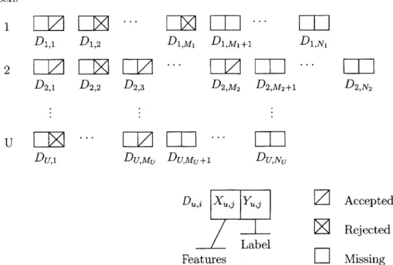
3.1.2 Dataset specification

A meeting request is labelled if the user has chosen whether to accept or reject the

meet-ing. In the meeting acceptance task, there are U users, U

e

that are labelled. Then XU A (Xu,1, Xu,2,..., Xu,MJ) denotes this user's labelled meeting requests and Xu- ' (Xu,Mj+1,. , Xu,Nj) denotes the unlabeled meeting requests, where

2_{A fair question to ask is whether the features I have chosen to use can be automatically extracted from} raw data. If not, then the system is not truly autonomous. Most of the features I inherited from the

CALO formulation can be extracted automatically from meeting requests served by programs like Microsoft

Outlook. Others, like the feature that indicates whether the requester is the user's supervisor, rely upon the knowledge of the social hierarchy in which the user is operating (i.e. the organizational chart in a company, chain of command in the military, etc). Fortunately, this type of knowledge remains relatively fixed. Alternatively, it could be learned in an unsupervised manner. Other features, e.g. the feature that describes the importance of the meeting topic from the user's perspective, would need to be provided by the user or learned by another system.

Users 1-P

LiE

D

D2,

DIZ

D

,

D

,

D

,

u

LZ

Du,

Du,i IXu,j Yujg

Label Features

Z

Accepted

Rejected

LI

Missing

each Xu,= (Xuj,1, Xu,j,2, - - -, Xu,J,F) is a vector composed of F features, the i-th feature,

i E {0, 1 . _{F}, taking values from the finite set Vi. Together, the concatenation of XUj}

and Xu- is written Xu, denoting the entire collection of meeting requests. Similarly, let

Yu+ A (Y, Yu,2,... ,Yu,M) denote the labels for the Mu labelled meeting requests. We

will write Y- to denote the Nu - Mu unknown labels labels corresponding to XU. Each Yu,i E {accept,reject} = 1,O}. For j E {,2,... , Mu}, Du = (Xu,j, Yu,) denotes the features and label pair of the j-th labelled meeting request. Then, D+ A (Xl, Y+) the

set of all labelled meeting requests for the u-th user. By omitting the subscript indicating the user, D+ represents the entire collection labelled meeting requests across all users. The same holds for X- and Y-.

Having defined the meeting acceptance task, we now turn to specifying how we will evaluate candidate models.

3.2

Evaluating probabilistic models on data

Each of the models I evaluate are defined by a prior distribution P(O) over a common, pa-rameterized family of distributions P(DJe). From a Bayesian machine learning perspective, the prior defines the hypothesis space by its support (i.e. regions of positive probability) and our inductive bias as to which models to prefer a priori.3 After making some observa-tions, D, new predictions are formed by averaging the predictions of each model according to its posterior probability, P(OID).

In the classification setting, the goal is to produce optimal label assignments. However, without a particular loss function in mind, we must justify another metric by which to evaluate candidate models. Since the true distribution has the property that it can perform optimally with respect to any loss function, in some sense we want to choose metrics that result in distributions that are "close" to the true distribution.

In this thesis, I use two approaches to evaluate proposed models, both of which can be 3

In the non-Bayesian setting, priors are used to mix predictions from the various models in a family.

After data is observed, the prior is updated by Bayes rule, just as in the Bayesian case. This "mixture approach" was first developed in the information theory community and shown to be optimal in various ways with respect to the self-information loss, or log-loss, as its known in the machine learning community. Consequently, the log-loss plays a special role in Bayesian analysis for model averaging and selection.

actual label

yes no

predicted yes true positive (tp) false positive (fp) label no false negative (fn) true negative (tn)

Table 3.1: Confusion Matrix: A confusion matrix details the losses associated each of the four possibilities when performing binary classification. The optimal decision is only a function of A1 = fp - tin and AO = f n - tp.

understood as empirical evaluations of two distinct classes of loss functions. The first class of loss functions evaluates label assignments, while the second class evaluates probability assignments. From the first class, I have chosen a range of asymmetric loss functions as well as the the symmetric 0-1 loss, which measures the frequency with which the most probable label under the model is the true label. From the second class, I have chosen the marginal likelihood (or log-loss, or self-information loss), which can be shown to favor models that are close to the "true" distribution (where distance is measured in relative entropy). Furthermore, I will show that the log-loss plays a central role in combining predictions from several models in a principled fashion.

3.2.1

Loss Functions on Label Assignments

When a probabilistic model is built for a classification setting, it is common for the model to be evaluated using a loss function representative of the intended domain. The symmetric 0-1 loss is a common proxy, and optimal decisions under this loss correspond to choosing the maximum a posteriori (MAP) label assignment. For this reason, the resulting classifier is sometimes referred to as the minimum-probability-of-error estimator. Intuitively, if the most probable label according to the model is often the true label, then the model is deemed a good fit. However, this intuition can be misleading.

Consider the following simple example involving a Bernoulli random variable X taking values in {0, 1}. Let us consider a set of models P, where each member p E P is a Bernoulli random variable with probability p. We will evaluate these models by computing their expected loss with respect to the true distribution, Pr[X = 1] = q. As we will see, the

(a)

1(b)

Figure 3-2: (a) Every loss function, (Ao, A1), induces a probability threshold, below which

models predict X = 0 and above which models predict X = 1. (b) Two thresholds, C1 and

C2, divide the space. The side of each threshold on which q lies defines the optimal decision for that threshold. Therefore, loss functions corresponding with the C1 threshold will prefer the pl model while those corresponding to C2 will prefer the P2 model.

Let A1 > 0 be the difference in loss between a false positive and true negative and

AO > 0 be the difference in loss between a false negative and true positive (see Table 3.1).

It then follows that the optimal decision for a model p e P is to predict X = 1 if

P > A , (3.1)

IAO

+

and X = 0 otherwise. Therefore, every loss function defines a probability threshold between

0 and 1, below which all models always predict X = 0 and above which all models predict

X 1. If the true probability q lies below the threshold, then the optimal decision is

X = 0, and vice versa (see Figure 3-2a). However, all models that lie on the same side

of the threshold will exhibit identical behavior and therefore, will be indistinguishable. In addition, it is obvious that, given any two models P1, P2 satisfying pi < q < P2, there exists

a pair of loss functions (specifically, thresholds) C1 and C2 such that, upon evaluation, C1 prefers p, and C2 prefers P2, regardless of how close either P1, P2 is to the true probability q (see Figure 3-2b). For example, consider the concrete setting where q = 0.51, p1 = 0.49 and P2 = 1.0. Then our intuition tells us to prefer pi but a symmetric loss function (A1 = AO)

will actually prefer the second model. If we shift the threshold beyond 0.51, then the first model is preferred.

The above example, while contrived, demonstrates an important point: optimizing for one type of loss function can result in model choices that conflict with common-sense in-tuitions about what constitutes a "good" fit. The above example, however, does suggest that it might be possible to use multiple loss functions to separate out the best model. Un-fortunately, as we consider more complex modelling situations, it will become increasingly difficult to design loss functions that will reveal which model should be preferred. Despite its drawback, this approach does result in easy-to-interpret values (e.g. percentage correct on a classification dataset), possibly explaining its widespread use. Besides its intuitive-ness, I have chosen to use this metric because it is a common metric in the classification literature. In addition, I will evaluate not only the symmetric loss function but a range of asymmetric loss functions in the hope of highlighting any differences between the models.

3.2.2

Loss Functions on Probability Assignments

The second approach I use in this thesis prefers models that assign higher likelihood to the data. By Gibbs inequality, the model q that maximizes the expected log-likelihood of data generated by some unknown distribution p,

Ep [log q~),(3.2)

is precisely q = p. This suggests that we evaluate the empirical log-loss of each of our candidate models. Choosing the best one corresponds to choosing the distribution that minimizes the relative entropy to the true distribution.

Despite the apparent simplicity of this approach, there are many implementation issues in practice. First and foremost, we cannot evaluate the expectation (3.2) because we do not know the true distribution p. Therefore, we instead calculate the empirical log-loss on the available dataset. The specifics of how we calculate the log-loss depends, at the very least, on how we intend to use the model class on future data. Each of the model classes we are evaluating is a parameterized family of distributions, P(DJe), with a prior distribution

P(1), where predictions are made by performing full Bayesian inference. If we imagine that

after every prediction we will receive feedback as to whether the correct decision was made, then the appropriate log-loss metric is the marginal likelihood, P(D) = f P(D; e)P(O) d1.

To see this, note that if D = (D1, D2,..., DpNr), then we can write

P(D)

P(D

) P(D

) P(D

ID1,

Often, this quantity is difficult to calculate as it involves a high-dimensional integral. How-ever, we will employ stochastic Monte-Carlo techniques that allow us to estimate it efficiently (Neal, 1993).

In the Bayesian setting, we can think about the question of future performance in a fundamentally different way. Surprisingly, we will find that the marginal likelihood is once again the metric of interest. Instead of choosing a model with which to make predictions, we can combine the predictions of several models together. Intuitively, the more we trust a