Simulation of the pressure field beneath a turbulent boundary layer using realizations of uncorrelated wall plane waves

1

Simulation of the pressure field beneath a turbulent

boundary layer using realizations of uncorrelated wall plane

waves

Laurent Maxit 5

Univ Lyon, INSA-Lyon, LVA EA677 Laboratoire Vibrations- Acoustique Bât. St. Exupéry, 25 bis av. Jean Capelle

F-69621 Villeurbanne Cedex, France laurent.maxit@insa-lyon.fr 10

Abstract

This paper investigates the modelling of a vibrating structure excited by a turbulent boundary 15

layer (TBL). Although the wall pressure field (WPF) of the TBL constitute a random excitation, the element-based methods generally used for describing complex mechanical structures consider deterministic loads. The response of the structure to a random excitation like TBL is generally deduced from calculations of numerous Frequency Response Functions. The result is that the process requires costly computational resources. To tackle this issue, an efficient 20

process is proposed for generating realizations of the WPF corresponding to the TBL. This process is based on a formulation of the problem in the wave-number space and the interpretation of the wall pressure field as uncorrelated wall plane waves. Once the WPF have been synthesized, the local vibroacoustic responses are calculated for the different realizations and averaged together in the last step. A numerical application of this process to a plate beneath 25

a TBL is used to verify its efficiency and ability to reproduce the partial space correlation of the excitation. Finally an application on a stiffened panel modelled with the finite element method is proposed to illustrate the interest of the proposed process.

Running title: Numerical synthesis of random pressure field 30

2

I.

INTRODUCTION

Structures excited by the turbulent boundary layer (TBL) are very common in practical 35

applications. Cars, airplanes, trains and submarines may be excited by pressure fluctuations due to the turbulent flow caused by their movements. In order to reduce the noise radiated from or transmitted by these structures, it is important to understand at the design stage how the structure reacts to TBL excitation. It is then necessary to develop numerical tools to predict the vibration or the pressure radiated from the complex panels excited by the turbulent flow. This 40

topic has been the purpose of many works in the literature and it remains an important research topic. To be convince, the reader can find a recent state of the art on this topic in the book [1] published after the FLINOVIA symposium held in 2013 at Roma.

Usually, the calculation process is decomposed into 3 steps: 45

- First, a hydrodynamic model is used to estimate the TBL parameters (convective velocity, boundary layer thickness, wall shear stress, etc.) over the surface of the structure on the basis of its geometry and the flow conditions.

- Second, the spectrum of the wall pressure fluctuations is evaluated from the TBL parameters estimated previously and by using one of the models proposed in the literature. 50

Some of them are expressed in the space - frequency domain (like the well-known Corcos model [2]), whereas others are in the wavenumber - frequency domain (like the equally well-known Chase [3] and Smolyakov [4] models). Discussions on different models and comparisons with experiments can be found in [5-8] for the Auto Spectrum Density (ASD) function and in [8-10] for the normalized Cross Spectrum Density (CSD) function.

55

- Finally, a vibro-acoustic model is used to estimate the response of the structure to the pressure fluctuations.

Many studies were carried out in the past to develop this type of calculation process for predicting the vibro-acoustic response of structures excited by fully developped TBL. The 60

former ones concerned generally simple plates excited by a turbulent flow. In the end of the 60th, Strawderman [11] gave a review of existing models (at this period) of finite and infinite plates under turbulence. Although neither the finite nor infinite model agrees wholly with the experimental results, he indicated that the vibration statistics computed from the finite plate model are in better agreement with the experimental results than those computed from the 65

3 infinite panel model. He also investigated with Christman [12] the effect of heavy fluid loading on the vibratory response. Davis [13] proposed a space integration method including the light fluid loading effect to estimate the power density functions of the displacement of the finite plate and of the radiated acoustic pressure. Graham [14] reviewed statistical models of the boundary layer and investigated the more specific case of aircraft statistical models of TBL. 70

The response of a finite panel under boundary layer excitation was determined by using the modal superposition method and a wavenumber integration technique. For naval applications, Ko and Schloemer [15, 16] proposed a method for evaluating the transmitted flow noise received by a rectangular hydrophone embedded in an infinite extended viscoelastic layer. The wavenumber filtering effects of both the elastomer layer and the rectangular hydrophone were 75

highlighted by their approach. Mazzoni [17] proposed a deterministic model to approximate the response of an elastic rectangular plate at a low Mach number. The approximation was based on the observations of numerical studies showing that the subconvective region of the turbulent excitation power spectrum contributes significantly to the response of the panel. Rumerman [18-20] derived different expressions giving broad band estimations of the acoustic power 80

radiated from a ribbed plate excited by TBL. He assumed a wavenumber-white pressure excitation and that the ribs radiated independently, that leads the formulations to be more accurate in the high frequency domain. Recently, Ciappi and al. [21] studied numerically and experimentally the response of two composite panels under TBL excitation for nearly subsonic flow conditions. They use literature empirical models for the WPF with the input date obtained 85

from the analyses of experimental wall pressure data. The comparison between finite element and experimental results showed a good agreement between the different results.

For the prediction of the vibratory response of complex panels under TBL excitation, the element-based methods considering deterministic harmonic excitations are generally 90

considered for describing the vibro-acoustic behavior of the panel. Finite Element Modeling (FEM) can be used for a pure structural problem whereas FEM coupled with Perfectly Matched Layers (PMLs) [22], the Boundary Element Method (BEM) [23], or the Infinite Element Model (IEM) [24] can be used for an acoustic radiation problem. The coupling between the statistical model used to describe the wall pressure fluctuations and the deterministic vibroacoustic model 95

represent a difficulty in the calculation process described above. Generally, this coupling is established thanks to a formulation of the random excitation problem in the frequency-space domain [25]. The ASD function of the system response (i.e. structure acceleration, acoustic pressure) at a receiving point is then linked to the CSD function of the wall pressure fluctuations

4 through Frequency Response Functions (FRFs) [24]. These FRFs are defined between the 100

receiving point and a set of points distributed on the excited surface. In order to correctly describe the partial correlation of the excitation, it is necessary to consider a large number of points on the excited surface and compute a large number of FRFs [24-25]. A study can be found in [26] which highlights the issues induced by the transformation of the pressure distribution into discrete locations (i.e. nodes), in particular the aliasing effect. Hong and Shin 105

[25] examined in details the maximum mesh size required for reliable finite element analysis. They showed that the mesh size should be defined under consideration of the spatial distribution of the CSD function of the WPF in addition to the dynamic characteristic of the considered structure. This may lead to consider a very fine finite element mesh and it results that the finite element calculations are both time and memory consuming.

110

Different alternatives have been proposed for overcoming these drawbacks. Ichchou et al. [27] were developed an equivalent “rain on the roof” excitation model for the high frequency range which largely simplified the Finite Element calculations. Hong and Shin [25] proposed an uncorrelated loading model of the WPF which was based on the compensation of the wall 115

pressure correlation lost due to the coarse mesh. A good accuracy with an exact solution was obtained with this approach on a simply supported beam. The proposed loading model can also be applied on more complex structures. In the same time, De Rosa and Franco [28] proposed a scaling procedure in order to reduce the computation cost which can be induced by a high modal density. It consists to reduce the dimensions not involved in the energy transmission whereas 120

the damping is increased in order to keep the same dissipated energy. The same authors and others [29] have also analyzed scaling laws from experimental data involving four plates in air or in water flow. More recently, the same team [30] proposed a frequency modulated pseudo-equivalent deterministic excitation. This approach named PEDEM is derived from the pseudo-excitation method [31-32]. This latter involves a modal decomposition of the load matrix related 125

to the CSD function of the WPF and it converges to the exact response if all the eigensolutions are considered. Different PEDEM approximations were studied for overcoming the drawback of the modal decomposition of the load matrix at each frequency step. The approximations depended on the considered frequency ranges (i.e. low, mid or high) which could be identified with a general criterion given by the authors. They were validated on a chain of linear oscillator 130

and on a flexural plate. Another type of approaches [24, 33] which has been developed recently consists in synthetizing realizations of the wall pressure fluctuations corresponding to the CSD function in the frequency-space domain. The process is based on a Choslesky decomposition

5 of the wall pressure CSD matrix [34]. Once the pressure fields corresponding to the different realizations have been obtained, the vibroacoustic model is used to calculate the system 135

response at the receiving point for each realization, separately. The response to the TBL excitation is finally deduced by an ensemble average on the different realizations. With this process, the number of load cases considered in the vibroacoustic calculations corresponds to the number of realizations, which is generally much lower that the number of FRFs considered with the standard approach described above. This is the advantage provided by this approach. 140

However, it always requires a fine finite element mesh of the panel for frequencies above the hydrodynamic coincidence frequency and the Choslesky decomposition is time consuming. In order to tackle these issues, this paper proposes an alternative process to the ones described in [24, 33]. It is based on a formulation of the random excitation problem in the frequency-wavenumber domain and the interpretation of the wall pressure field as uncorrelated wall plane 145

waves. Realizations of the WPF are directly generated from an analytical expression depending on the wavenumber-frequency spectrum of the WPF. The Cholesky decomposition is then not be required. For each realization, the panel response induced by the deterministic WPF (of the considered realization) can then be estimated from a low-frequency deterministic vibro-acoustic model of the panel. For instance, it can be achieved by using a finite element model 150

when dealing with a complex panel. The stochastic response of the panel is then obtained from an ensemble average of the different panel responses. The interest of this type of approach is that it requires a relatively small number of realizations for estimating the stochastic response of the panel. This point will be studied on the basic case of a simply supported plate. Moreover, we will highlight how in some situations, the well-known filtering effect of the panel [35, 36] 155

can be considered in the process in order to reduce the mesh size of the panel. The accuracy of the proposed process will be studied in function of the WPF model (i.e. Corcos or Chase), the convective velocity of the flow and the panel thickness. A stiffened plate modelled with the finite element solver MSC/NASTRAN will also be considered to illustrate the interest of the present approach for practical application.

160

The paper is organized as follows:

- Section 2 gives a description of the problem considered and presents the outlines of its mathematical formulation in the frequency-wavenumber space;

- Section 3 introduces the concept of uncorrelated wall plane waves and proposes the 165

6 - The numerical process for estimating the panel response to TBL excitation is

summarized in Sec. 4.

- Then, in Sec. 5, numerical applications are proposed for a basic case of studying the influence of different parameters on the accuracy of the approach proposed.

170

- Finally, before the concluding remarks, an application on a stiffened plate is proposed in Sec. 6.

II.

VIBRATING

PANELS

EXCITED

BY

RANDOM

PRESSURE FLUCTUATIONS

175

Presentation of the problem

Fig. 1. Baffled simply supported plate excited by a homogeneous and stationary TBL. 180

Let us consider a baffle panel of surface p excited by a TBL as shown in Fig. 1. We assume that the TBL is fully developed, stationary, and homogeneous over_p. Moreover, the panel and the boundary layer are assumed to be weakly coupled. It is then assumed that the vibration of the plate does not interfere with the wall pressure. The spectrum of the wall pressure fluctuations over a rigid surface can then be considered for charactering the panel excitation. 185

This can be estimated from the parameters characterizing the turbulent boundary layer (i.e. convective velocity, U ; boundary layer thickness; wall shear stress), and one of the wall _c pressure models proposed in the literature [2-7]. The space-frequency cross spectrum of the

Lx

h Ly

7 wall pressure fluctuations STBL_pp



xx,



may be written on the specific form proposed by Graham [10] and reused by different authors ([5, 37]):

190





 







   , , 2 x x x x            TBL pp c pp TBL pp S U S S , (1) where: - Spp

 

 (in Pa

2_{/Hz) is the Auto Spectrum Density (ASD) function of the WPF} depending on the angular frequency



, and;

- S_ppTBL



xx,





(in rad2/m2)) is the normalized Cross Spectrum Density (CSD) function of the WPF depending on the spatial separation between two points, xx, and the 195

angular frequency.

This form can be used with different models for the ASD function and for the normalized CSD function, independently one from each other. For example, the Goody [6] or Rozenberg [7] models can be used for the ASD function whereas the Corcos [2] or Chase [3] models can 200

be considered for the normalized CSD functions.

It is assumed that the panel has a linear vibroacoustic behavior that can be represented by a deterministic model (like FEM). It may be complex. That is to say, for example, that it could be made of different layers of different materials. It could also be stiffened by ribs on the side 205

opposite the flow.

The goal for us consists in estimating the vibrations of this panel when it is excited by the wall pressure fluctuations induced by the TBL. In the next section, we give the outlines of the formulation of this problem in the frequency-wavenumber space. Details of the formulation can 210

be found in the literature [38-40].

Mathematical formulation

 

~x,

b

p represents the wall-pressure fluctuations due to the TBL on the plate at pointx as a function of time t. The plate acceleration at point x due to wall-pressure fluctuations,



 

x,t , 215

8

 

_{ }



  

      p d d p t h t x x _b x x x, ,~,  ~,  ~   , (2)

where h_



x, x~,t



is the acceleration impulse response at point x for a normal unit force at point

x

~_.

As the turbulent flow induces a random process, the plate response is characterized by the auto correlation function of the acceleration, R_. Assuming that the process is stationary and 220

ergodic (i.e. expectation replaced by the limit of a time average), R_can be written as:

 

_

  



     2 / 2 / , , 1 lim , T T T _T t t d t R x  x  x  . (3)

By introducing (2) in (3) and taking the time Fourier transform of the result, we obtain the Auto Spectrum Density (ASD) of the acceleration at pointx(see details in [38-40]):

 

_{ }







  

    p p d d H S H S x x x TBLpp x x x x x x ~ ~ ~ , ~ ~ , , ~ ~ ~ , ~ , , *      , (4) where











     h t e dt

H x,~x,  x,x~, jt is the Frequency Response Function (FRF) in terms of acceleration at point x for a normal force at point ~x and the asterisk denotes the complex 225

conjugate.

Now, let us consider the space Fourier transform of the wall pressure spectrum,



TBL_pp

 

k,



. This is related to the wall pressure spectrum in the physical spaceSTBL_pp



xx,





by



_{x x}



 

_k kx x _k d e STBL_pp TBL_pp i  



   . 2 , 4 1 ,     . (5) 230

Introducing Eq. (5) in Eq. (4) gives

 

_

  



  k xk k x H d S ₂ TBL_pp , ~ , , 2 4 1 ,      _  , (6) with





_





  p d e H H~_ x,k, _ x,~x, jk~x ~x. (7)

9







 , , ~ k x

H is generally called the sensitivity function [41]. The interpretation of Eq. (7) indicates that this quantity corresponds to the acceleration at point x when the panel is excited by a unit wall plane wave of wavevector k (i.e. by a WPF

 

j _p

b e

p ~x  k~x,x~ ).

235

In Eq. (5-6), improper integrals exist over the wavenumber space. In the following, it is assumed that they can be approximated by considering the rectangular rule and by truncating and regularly sampling the wavenumber space. The criterion for defining the cut-off wavenumbers and the wavenumber resolutions will be discussed later. However, it should be 240

underlined here that the cut-off wavenumbers can be different between Eq. (5) related to the wall pressure and Eq. (6) related to the panel vibration due to the well-known filtering effect of the panel [35]. p and denote the sets of wavenumbers selected to estimate Eq. (5) and (6), respectively. Thus the following can be written:





 

  k k x x  



k x x     p i TBL pp TBL pp e S        . 2 , 4 1 , , (8)

 

_

  



          x _  k  xk  k 2 2 , , ~ , 4 1 , H S TBL_pp , (9)

where krepresents the wavenumber resolutions. 245

The outlines of the formulation for estimating the vibratory response of the panel have been presented here. One can emphasize that these developments can be easily adapted for evaluating the noise radiated by the panel (see the details of the formulation in [38-40]). It is however outside the scope of the present paper which focus on the synthetize of the WPF and the 250

prediction of the panel vibration.

III.

UNCORRELATED WALL PLANE WAVE FIELD

The basic idea of the proposed approach is to represent the TBL pressure CSD function as the result of a combination of uncorrelated wall pressure plane waves. This approach may be related 255

to room acoustics, where a diffuse field can be represented by summing the effect of an infinite number of acoustic plane waves originating from all spatial directions and having the same amplitude [42].

This section is organized as follow: we define first the concept of uncorrelated wall plane waves. Then, we establish the link between the uncorrelated wall plane waves and the TBL 260

10 excitation. Finally, we propose a process for synthetizing realizations of the WPF induced by uncorrelated wall plane waves. As the uncorrelated wall plane waves can be representative of the TBL excitation when the wave amplitudes are correctly defined, the process which will be described in this section will permit to synthetize realizations of the WPF induced by a TBL excitation.

265

Definition

Let us define the concept of uncorrelated wall plane waves. One recalls that the term wall plane wave refers to the blocked pressure acting on a panel surface varying spatially as 270

p j

ekx,x where k is the wavevector of the wave considered. It is assumed that this wave has a stochastic amplitude. The blocked pressure induced by a wall plane wave  of wavenumber



k can then be written

 



 

k x



x    j e t A t p , Re , ₍₁₀₎

where A_

 

t is a random variable.

This wall plane wave is clearly a surface wave in the sense that it is only defined at the surface 275

of the panel. Moreover, we underline that the wavevector kmay be arbitrary in the 2-D real space kℝ2. It does not depend on the acoustic propagation as it is the case for an acoustic plane wave.

The pressure CSD function corresponding to this wall plane wave is therefore:





 

k xx x x   _{ }       j A A p p S e S , , ₍₁₁₎

where S_AA

 

 is the ASD function of the wave amplitude. 280

Now, let us consider a set of Uncorrelated Wall Plane Waves (UWPW) of wavenumbers

 

  ,

k . The total blocked pressurep

 

x,t is given by:

 

_

 

     t p t p x, x, . (12)

As the wall plane waves are assumed to be uncorrelated, the CSD function between the amplitudes of two different waves is null: S_AA

 



0 if







. Hence the CSD function of the pressure induced by this set of uncorrelated wall plane waves is therefore:

11





_

 

            





k x x x x _AA j UWPW pp S e S , . (13)

Uncorrelated wall plane wave field and TBL excitation

Now let us establish a link between the UWPW and the TBL excitation. To do that, one considers a set of UWPW defined such that_p and the ASD functions of the wave 290

amplitudes are given by:

 



 

         ₄ , , 2 k k TBL pp A A S . (14)

By introducing Eq. (14) in Eq. (13) and by comparing the results with Eq. (8), it can be seen immediately that SUWPW_pp



xx,





STBL_pp



xx,





. This clearly demonstrates that the TBL excitation can be represented as a superposition of uncorrelated wall pressure plane waves. 295

It is possible to verify that this representation of the TBL excitation remains consistent with the panel response. Indeed, if we consider a set of UWPW with_, the ASD function of the panel acceleration in response to the set of UWPW may be written as:

 

_{ }





 





                  x, H~ x,k ,S  H~ x,k , SUWPW _AA , (15)

which is simplified because the wall plane waves are uncorrelated:

 

_

 





             2 , , ~ , xk x S H SUWPW _AA . (16)

When defining the wave amplitudes by Eq. (14), the direct comparison of Eq. (16) and Eq. 300

(9) gives SUWPW

 

x,



STBL

 

x,



.

In conclusion, the TBL excitation can be represented by a set of UWPW when the wave amplitudes are defined with Eq. (14).

Realizations of uncorrelated wall plane wave fields

Let us now define a process for synthetizing realizations of the WPF induced by UWPW. A set 305

of UWPW as defined in the previous section constitutes a random excitation. One way of approximating it is to consider different realizations of the random pressure field. Using the physical interpretation of uncorrelated wall plane waves, it is possible to define the wall pressure field of the kth realization, pk

 

x, by,

12

 

 

kx x         j j A A k e e S p



k    , , (17)

where



k, are random phase values uniformly distributed in



0, 2





.

310

In this expression, the terms

k

j

e express the fact that the wall plane waves are uncorrelated and the terms S_AA

 

 represent the wave amplitudes. The root square of the ASD function of the wave amplitudes is used to counteract the second-moment related to the ASD function. It can be easily demonstrated that the CSD function of the wall pressure corresponding to an infinite number of these realizations, S_ppS



xx,





, corresponds well to the CSD function of the 315

uncorrelated wall pane wave field, SUWPW_pp



xx,





. Indeed, SS_pp



xx,





can be written by definition:





 

 

k j j A A j j A A S pp E S e e S e e S k k _             





kx kx x x _{ }   _{ }         , , (18)

whereE

 

_krepresents the ensemble average over the realizations and the upper bar denotes the complex conjugate of the complex number.

320

By rearranging the different terms,





 

 

 

 

 k j j A A A A S pp k k e E e S S S _{   }                   



   kxk x x x , , (19)

and by considering an infinite number of realizations,





 













 

otherwise,

,

0

,

if

,

1





    k j k k

e

E

(20) we obtain S_ppS



xx,





SUWPW_pp



xx,





.

This demonstrates well that when considering an infinite number of realizations, the CSD 325

function of the WPF defined by Eq. (17) is equivalent to the CSD function of the uncorrelated wall pane wave field.

To summarize this section 3, one can emphasize that: (a), the TBL excitation can be represented by a set of uncorrelated wall plane waves when the wave amplitudes are defined 330

by Eq. (14); (b), Realizations of the random pressure field corresponding to a set of uncorrelated wall plane waves can be obtained using Eq. (17); (c), The CSD function of the WPF

13 corresponding to these realizations converge to the CSD function of the set of uncorrelated wall plane waves when the number of realization tends to infinity.

It results that realizations of the random pressure field corresponding to a TBL excitation 335

can be obtained by using Eq. (17) when the wave amplitudes are defined by Eq. (14). The CSD function of the WPF corresponding to an infinite number of realizations is then equal to the CSD function of the TBL excitation. An infinite number of realizations of the WPF as described previously are then equivalent to the TBL excitation. In consequence, the response of the panel under TBL excitation can be estimated from the response of the panel excited by the WPF 340

corresponding to these realizations. In practice, a finite number of realizations K will be considered to approximate the TBL excitation. The accuracy of the calculation process summarized in section 4 will be studied in section 5 in function of the number of realizations.

IV.

PROCESS FOR ESTIMATING THE PANEL RESPONSE

345

FROM THE WALL PRESSURE REALIZATIONS

The following is a description of the numerical process for estimating the panel response to a TBL excitation from the realizations of the uncorrelated wall plane wave field. This process is directly derived from the previous section. One has seen that the realizations of the WPF defined 350

by Eq. (17) with Eq. (14) are representative of the WPF of the TBL excitation. The proposed process consist then to estimate the panel response to the WPF of each individual realization and then to average the obtained panel responses over the different realizations.

Let us consider a deterministic vibroacoustic model of the panel in order to estimate the 355

panel response to deterministic load cases. This model can be an analytical model for an academic structure or an element-based model for a complex panel (as it will be illustrated in section 6 for a stiffened plate represented by a finite element model within the MSC/NASTRAN code).

360

The numerical process proposed can be decomposed into three steps:

- The first step consists in calculating the WPF of K realizations of the uncorrelated wall plane wave field representing the TBL excitation. It is carried out by using the formula (17) and considering the wave amplitudes defined by Eq. (14). When using an element-based method for describing the vibro-acoustic behavior of the panel, the WPF should be applied to the nodes 365

14 of the mesh belonging to the interaction surface between the panel and the flow. For the node i of this set of nodes, the pressure corresponding to the kth _{realization (deduced from Eq. (14) and} (15)) is given by:









 i k y i xx k y k j y x y x TBL pp i i k e k k k k y x p                



 ₂ 4 , , , , , (21) where:

- x and y represent the axis in the streamwise direction and the crosswise direction, 370

respectively;

-



k ,_x k_y



are the coordinates of the wavevectork ; _

-

 

x ,i yi are the coordinates of node i.

- k_xand k_y are the wavenumbers resolutions in the spanwise and streamwise directions, respectively, and;

375

-



_k, are random phase values uniformly distributed in



0, 2





;

- In the second step, the vibroacoustic model is used to estimate k

 

x, , the panel acceleration at point x when the panel is excited by the deterministic WPF, pk

 

x, calculated in the previous step. When an element-based model is considered, expression (21) is directly 380

used to prescribe the pressure on the nodes at the interface between the panel and the flow. A direct frequency analysis can then be performed for example to estimate the panel acceleration

k

 . This calculation is repeated for the different realizations k



1,...,K



. The number of load cases considered in the vibroacoustic simulations therefore corresponds to the number of realizations;

385

- Finally, in the last step, the ASD of the acceleration at point x is estimated by an

ensemble average of the acceleration responses, k

  

x, ,k1,...,K



estimated in the previous step:

 



   



k  K k k S E S x,   x, x, _1,..., . (22) 390

 

 S x,

S corresponds then to the ASD of the acceleration at point x induced by the WPF of

15 function of the WPF of the TBL excitation when K, S_S

 

x, converge to the ASD function of the plate acceleration at point x induced by the TBL excitation. In practice, a finite

number of realizations K will be considered to approximate the ASD function of the plate 395

acceleration. This will be studied in the next section.

V.

NUMERICAL APPLICATIONS

For evaluating the numerical process described in the previous section, we are going to compare 400

its results on a basic application case with the results obtained by a direct calculation of Eq. (9). In the following, the latter calculation is named the sensitivity function method whereas the numerical process described in section 4 is called the sampling method.

Presentation of the test case

405

The test case considered for this numerical application is composed of a rectangular thin plate simply supported along its four edges and excited by a turbulent air flow. This academic plate was chosen because the modal base can be obtained analytically and the vibratory response can be easily interpreted. The plate is made of aluminum and the flow direction is parallel to the longest edges of the plate (i.e. about the x-axis). The effect of the air on the plate vibrations are 410

neglected. The numerical values of the physical parameters considered for this nominal test case are given in Tab. 1. To study the influence of different parameters on the accuracy of the presented approach, one will be led to modify the physical parameters of the nominal case. This will be indicated in the text. For the sake of compactness, one limits however the study to the cases presenting a hydrodynamic coincidence frequency (i.e. frequency for which the flexural 415

wavenumber is equal to the convective wavenumber) lower than the higher frequency of interest (i.e. frequency for which the flexural wavenumber is equal to the convective wavenumber). In particular, one does not study the cases concerning by a frequency band of interest below the hydrodynamic coincidence frequency. For the nominal case, the hydrodynamic coincidence frequency is 86.7 Hz and the higher frequency of interest has been 420

16

Parameters Numerical value

Panel thickness h3mm

Panel length in the streamwise direction _1.5m x

L

Panel length in the crosswise direction Ly 0.9m

Panel Young’s modulus E67 109 _Pa

Panel Poisson’s ratio  0.34

Panel mass density  2700 kg/m 3

Panel damping loss factor  0.01 

Receiving point coordinates



_,

 

 _{0.133m,0.212m}



M M y x Convective velocity c U = 50 m/s TBL displacement thickness * _5.3mm Friction velocity * _2.6m/s u 425

Table 1. Physical parameters of the nominal test case.

Two different models of WPF will be considered in order to study the influence of the model on the accuracy of the results. From Eq. (1) and the definition of the space Fourier transform (5), the CSD function of the WPF in the wavenumber space TBL_pp can be written:

430





 









    , , , , 2 y x TBL pp c pp y x TBL pp k k U S k k        , (23)

where _ppTBL



k_x,k_y,



is the normalized CSD function of the WPF in the wavenumber space which is a dimensionless quantity.

The Corcos model is first considered because it provides an analytical expression of the CSD function both in the space-frequency domain



xx,





[2] and in the wavenumber-frequency 435

domain

 

k,



. The Corcos model is a semi-empirical model. Although the Corcos model is simple and it is frequently used in the literature, it has been pointed out by different authors that it may be deficient to represent accurately the subconvective domain of the WPF [44]. One can also notice that some improvements have been proposed recently to circumvent this issue [45]. We consider however the Corcos model in the following due its simplicity, without any 440

17 consideration on its ability to reproduce fairly the WPF induced by a TBL. The Corcos normalized CSD function of the WPF used in the following depends on the convective velocity given in Tab. 1 for the nominal case. It is given by ([10], [37]):





                                ₂ 2 2 2 1 4 , ,         y c y x c x y x y x TBL pp k U k U k k , (24)

with the Corcos’s parameters: _x 0.11, _y 0.77. 445

The second model of WPF considered for the numerical applications is the Chase model [10, 43]. It has been deduced from theoretical developments based on the Poisson equation and it depends on numerous empirical parameters. It is supposed to be more accurate in the low wavenumber region that the empirical models [45]. The Chase normalized CSD function of the WPF is expressed by Eq. (3.18) to (3.20) of Ref. [10]. The empirical constants given after these 450

equations in this reference are also considered in the present paper. This model depends on the TBL displacement thickness, the friction velocity and the convective velocity which are given on Tab. 1 for the nominal case.

For the sake of simplicity, the vibratory responses of the panel are normalized by 455

 

, 2         c pp U

S which makes it independent of the ASD of the WPF. In others words, this normalized response corresponds to the vibratory response of the panel induced by the WPF defined by the normalized CSD function, TBL



_x, _y,



pp k k (see Eq. (23)).

Numerical modelling

460

The vibratory response of the plate to a given pressure field,p_e



x, y,



can be easily estimated by using the modal expansion method. The modal angular frequency,  , the modal shape,_m,n

n m,

 and the modal mass, Mm,n, are given for each couple of non-null integers

 

m,n by:

2 2 ,                y x n m L n L m h D     ,

 

_              y x n m L n L m y x    _, , sin sin , 4 , y x n m L hL M  . (25)

where D is the flexural rigidity given by

 

₂ 3

1 12   Eh

18 For the modal expansion, the modes having a frequency in the extended angular frequency 465

band



0 ,3/2_max



are considered, where_maxrepresents the highest angular frequency of interest.

 







 m,n ℕ∗× ℕ∗/m_,n



0 ,3/2_max





denotes the set of modal order couples corresponding to

these modes.

To estimate the ASD function of the panel acceleration directly with Eq. (9), it is necessary 470

to estimate the sensitivity functions H~_ at point



x ,_M y_M



for each couple of wavenumbers

 

k ,x ky :





_









_

 



      n m mn mn mn M M n m y x n m y x M M j M y x k k k k y x H , 2 , , 2 , , , 2 , , , , , , ~         . (26) n m,

 represents the modal force given by

 

 

y n x m L L n m y jk x jk y x n m k k e x y I I x y y x  

 

 0 0 , , ,  ,  , where (27)

 

                              otherwise. , 2 1 , if , 1 1 2 2            jL L p k L p k e L p I x L jk p p ₍₂₈₎ 475

On the other hand, to estimate the ASD function of the panel acceleration with the numerical process described in Section 4, it is necessary to estimate k



x_M,y_M,



, the acceleration response at point



x ,_M y_M



induced by the wall pressure (17) corresponding to the kth realization:





_

  



_

 



      n m _{mn mn mn} M M n m k n m M M k j M y x F y x , 2 , , 2 , , , 2 , , ,          , (29)

where the modal forces are given by:

 

mn

 

x y j A A k n m S e k k F k , , ,       



  . (30)

The latter expression is well adapted for the present case for which we can calculate an 480

analytical expression of  (i.e. Eq. (27-28)). For a complex panel, the forced response or the _m,n mode shapes can be calculated by FEM and can be known at discrete points (i.e. the nodes of

19 the mesh). In the literature ([24-25], [28]), it has already been shown that the size mesh should be defined carefully for describing correctly the spatial variations of the WPF and for avoiding aliasing phenomenon [25]. In order to study the influence of this type of approximation in the 485

framework of the proposed approach, we also perform an approximation of the modal forces by considering a spatial discretization of the mode shapes by S points along the streamwise direction and R points along the crosswise direction. The modal forces for the kth realization can then be approximated by using the rectangular rule:



r x s y

 

r x s y



x y p F R r S s n m k k n m 



      0 0 , , , , , . (31) with R L x x  , S L y y  . 490

The spatial resolutions  and x



y

can be defined using a criterion based on the TBL characteristics or on the plate characteristics. This point will be studied in section V.D.4.

Definition of the sets of wavenumbers

495

Before evaluating the sampling method, one defines the sets of wavenumbers which intervene Eq. (8) and (9) for the sensitivity method and in Eq. (17) and (21) for the sampling method. They were introduced as the results of the truncation and the sampling of the wavenumber space in order to approximate the integrals of Eq. (5) and (6).

500

The criterion for defining the cut-off wavenumbers in the streamwise and the crosswise directions should be defined such that the significant contributions of the integrands of these equations are taken into account well.

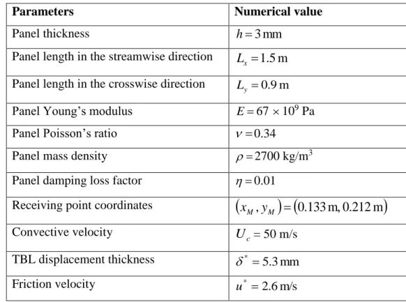
- Definition of the cut-off wavenumber in the streamwise direction 505

To highlight the different contributions in the wavenumber space for the nominal test case, we plotted on Fig. 2 the two quantities which intervene in the integrands of Eq. (5) and (6). They are expressed as a function of the streamwise wavenumber k , and the frequency f _x







2



f



, in the case of the crosswise wavenumber ky, fixed at 0. 510

20 Fig. 2a shows the normalized CSD function of the wall pressure spectrum of the Corcos model. It exhibits the highest values for wavenumbers close to the convective wavenumber k _c. Furthermore, in Fig. 2b, the highest values of the sensitivity functions (calculated with Eq. (26)) can be observed for frequency and wavenumbers close to the modal frequencies and the modal wavenumbers in the streamwise direction, respectively. To illustrate this, we have indicated the 515

modal frequencies and the modal wavenumbers of the first 10 modes of the plate in Tab. 2. The frequency and wavenumber of the highest amplitudes in Fig. 2b correspond well to the modal frequency f_m,n and the modal wavenumbers k of the plate modes with n=1. It should be _m emphasized that only these particular modes have the most significant contributions in the sensitivity functions shown in fig. 2b because the crosswise wavenumber is equal to 0 for this 520

figure (i.e. k_y 0). Whatever the case, it can be however concluded that the highest values of the sensitivity functions can be observed for wavenumbers below or close the natural flexural wavenumber of the plate k_f   h D (see Fig 2b).

(a)

(b)

Fig. 2. (a), The normalized CSD function of wall pressure spectrum given by the Corcos model, _ppTBL



k_x,0,



(dB, ref. 1); (b), The sensitivity function of the plate at point



x ,_M y_M



, 525





2 , 0 , , ,   xM yM kx H (dB, ref. 1).

21 n m f , (Hz) m x m L m k   (m-1) _n y n L n k   (m-1) 12.1 1 2.09 1 3.49 21.7 2 4.18 1 3.49 37.7 3 6.28 1 3.49 38.7 1 2.09 2 6.98 48.4 2 4.18 2 6.98 60.1 4 8.37 1 3.49 64.4 3 6.28 2 6.98 83.2 1 2.09 3 10.47 86.8 4 8.37 2 6.98 88.9 5 10.47 1 3.49

Table 2. Modal information for the first ten modes of the plate: f_m,_n , the modal frequency



m,n2fm,n



; m, n, the modal orders in x and y directions, respectively; k , m k , the modal n 530

wavenumbers in the x and y directions.

For defining the set of wavenumbers _p related to the wall pressure field (i.e. Eq. (8)), the cut-off wavenumbers should be defined only from the characteristics of the wall pressure spectrum (as the blocked pressures are independent of the panel). The truncation of the 535

wavenumber space should include the convective ridge in the streamwise direction. Then, one defines the cut-off wavenumber by:

max c p

x k

k  , (32)

wherek_cmaxis the convective wavenumber at the higher frequency of interest and  is a margin coefficient greater than one. In the following,  1.2 will be considered.

540

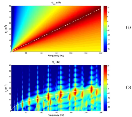
For defining the set of wavenumbers _ related to the panel acceleration, the truncation of the wavenumber space should be done by considering, both, the excitation characteristics and the panel characteristics. Fig. 3a shows the result of the product between and the wall pressure spectrum (i.e. Fig 2a) and the sensitivity function (i.e. Fig 2b). It should be underlined that this product appears in the summation of Eq. (9) to evaluate the ASD function of the plate 545

22 acceleration. It can be observed on Fig. 3a that the contribution of the convective domain is negligible. This is due to the well-known filtering effect of the pressure fluctuations by the panel [35, 36]. Thus, for this case, the truncation of the wavenumber space in the streamwise direction can be achieved without considering the convective ridge. The cut-off wavenumber in the streamwise direction used to define the set of wavenumbers _ in Eq. (9) or in Eq. (17) 550

can then be given by:

max 1 f x k k  , (33) where max f

k is the convective wavenumber at the higher frequency of interest.

(a)

(b)

Fig. 3. Values of the product between the sensitivity function and the wall pressure spectrum,



 



2 , 0 , , , , 0 ,   TBL _{x  M M x}

pp k H x y k (i.e. integrand of Eq. (6), dB, ref. 1). Results for two models of 555

wall pressure spectrum: (a), Corcos model; (b), Chase model. Dashed line: convective wavenumber; Solid line: flexural wavenumber.

It should however be mentioned that it is not a general result. The filtering effect of the structure is not always enough important to vanish the contributions of the convective ridge. It 560

23 depends in particular on the frequencies of interest [35], the panel boundary conditions [36], and the considered model of the WPF. This latter dependency is highlighted on Fig. 3b showing the same type of results than Fig. 3a when considering the Chase model. One can observe that the contributions of wavenumbers above the flexural wavenumber are more important with the Chase model than for the Corcos model. This is due to a stronger decrease of the CSD function 565

in the low wavenumber domain of the Chase model compared the Corcos model. For the considered case, the criterion defined by Eq. (33) may be in its limit of validity with the Chase model. This will be verified in the section 5.D.1 In the case of the filtering effect of the structure is not dominant, the criterion (34) based on the TBL characteristics should be applied to estimate the panel response:

570 max 2 c p x x k k k   . (34)

- Definition of the cut-off wavenumber in the crosswise direction

For the crosswise direction, it can be observed in general that the wall pressure spectrum decreases monotonically when the crosswise wavenumber k_yincreases. The cut-off wavenumber p

y

k related to the wall pressure field (i.e. Eq. (8)) has been fixed at 300rad/m1 575

with a trial-and-error process. For the panel response, the result of the product between the sensitivity functions and the wall pressure spectrum is dominated by the wavenumbers below or close to the natural flexural wavenumber of the plate (results not plotted here). The cut-off wavenumber in the crosswise direction can then be defined as the one in the streamwise direction: 580 max f y k k  . (35) - Wavenumber resolutions

The wavenumber resolutions in the two directions should be defined such that they correctly represent the spatial variations in the wavenumber space of the wall pressure spectrum and the sensitivity function. The analytical expression of the sensitivity functions for the panel 585

considered (i.e. Eq. (26-28)) gives an order of magnitude of these spatial variations (inversely proportional to the panel lengths) whereas the wall pressure spectrum varies relatively slowly as a function of the wavenumbers. In the following, the wavenumber resolutions are then fixed at 0.25 rad/m, independently of the frequency. For a more complex panel, a trial and error process can be used to fix these parameters.

24

Analysis of results

1. The sensitivity method

The ASD function of the panel acceleration at the receiving point M has been evaluated with 595

the sensitivity method for the nominal test case. Calculations have been performed for the two cut-off wavenumber criterions (33) and (34) (i.e. kx124.3rad/mand 45.2rad/m,

2 



x

k

respectively) and for the two models of WPF described in section 5.A (i.e. Corcos and Chase models). The results are plotted on Fig. 4 in function of the frequency. For the Corcos model, a very good agreement between the two calculations are observed on the whole frequency band 600

of interest. This confirms that the structure filters sufficiently the convective ridge of WPF in order that this latter can be neglected. For the Chase model, the agreement between the two calculations is very good up to around 200 Hz. Above this frequency, the calculation considering the criterion (33) underestimates slightly the panel response. A difference of 2.5 dB can be observed at 300 Hz. This can be explained from the observations made on Fig. 3b in 605

the previous section. These results highlights well that the criterion (33) should be used with carefully. We reach its limit of validity for the present case with the Chase model. However for the present case, the prediction remains globally a correct estimation of the plate response.

In the following, the results of the sensitivity method using the criterion (34) will be used as 610

25 (a)

(b)

Fig. 4. ASD function of the panel acceleration at the receiving point M as a function of the frequency, 10log₁₀



S_

 

M



(dB, ref. 1 m/s2/Hz0.5). Comparison of results obtained with the sensitivity function method with different criterion of the truncation of the wavenumber 615

space: Full line, criterion (34) based on the TBL characteristics; dash line, criterion (33) based on the plate characteristics. Results for two models of wall pressure spectrum: (a), Corcos

model; (b), Chase model.

2. Synthesis of the wall pressure field

620

The realizations of the wall pressure field are achieved using Eq. (17). By way of illustration, the WPF of two realizations at 300 Hz are given in Fig. 5 considering the Corcos model:

- The first one (Fig. 5a) has been obtained when the wavenumber set is defined with the TBL characteristics (i.e. _p). Spatial variations due to wave propagations in the 625

26 streamwise direction appear. The wavelength of these waves is around 0.2m, which correspond roughly to the convective wavelength (_c 2/k_c 0.16 rad/m at 300 Hz).

- The second one (Fig. 5b) considers the wavenumber set defined from the panel characteristics (). In particular, the criterion (33) is applied to define the cut-off wavenumber in the streamwise direction. One can notice that the spatial variations present 630

higher wavelengths and the amplitudes are lower than in Fig. 5a. This is directly due to the truncations of the wavenumber space which is more restrictive when considering the panel characteristics than the TBL characteristics. The WPF of Fig. 5b does not represent the convective ridge of the TBL. It explains why the amplitudes are lower. However, it represents the part of the pressure field induced by the TBL that contributes to the panel vibration. 635

(a)

(b)

Fig. 5. Two realizations of the WPF at 300 Hz obtained with Eq. (17): (a), using the wavenumber set defined with the TBL characteristics (i.e. _p); (b), using the

wavenumber set defined with the plate characteristics (i.e. _). 640

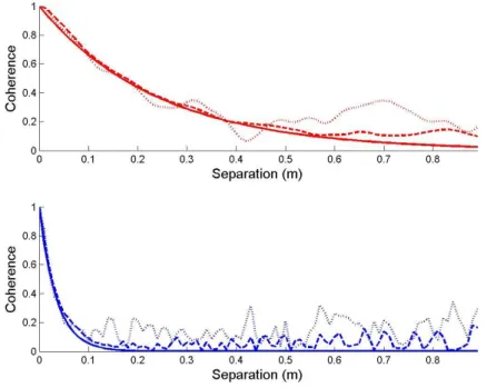
In order to study the WPF synthetized with Eq. (17), one will compare the spatial coherence estimated from the WPF of K realizations with the one given by the analytical expression of the

27 Corcos model. The spatial coherence between point x and x' can be estimated from K realizations by:







  





 

 

 





k  K k K k k K k k k p E p E p p E ,..., 1 2 ,..., 1 2 ,..., 1 , , , , , ,                   x' x x' x x' x . (36)

where pk

 

x, is obtained with Eq. (17). 645

The results of this equation for K=30 and K=900 are plotted in Fig. 6 for the streamwise and crosswise directions. It is clear that the small coherence length in the crosswise direction compared to the streamwise direction is well represented by the stochastic process even if only 30 realizations are considered. It can also be seen that a large number of realizations should be considered to correctly represent the small coherences corresponding to a relatively large 650

separation. This seems to indicate that a relatively large number of realizations should be necessary to represent the wall pressure fluctuations finely. However, as the panel filters the wall pressure fluctuations, it is not evident that a large number of realizations remain necessary to evaluate the panel response. This will be the subject in the next sections.

655

Fig. 6. Spatial coherence of the TBL pressure field as a function of the spatial separation in the streamwise direction (Upper) and in the crosswise direction (Lower). Full line, analytical

formula of the Corcos model; dotted line, numerical estimation considering 30 realizations; dash line, numerical estimation considering 900 realizations.

28

3. Results of the sampling method on the nominal test case

The process described in section 4 is applied to evaluate the ASD function of the panel acceleration at the receiving point. The nominal test case with the Corcos model and 30 realizations are considered. The cut-off wavenumber criterion based on the TBL characteristics 665

(34) is applied. For each realization, the panel acceleration has been obtained using the modal expansion Eq. (29-30). One recalls that the modal forces resulting of the WPF is then calculated analytically. To illustrate the process, one has plotted on Fig. 7 the results of the 30 realizations (grey line). One can observe a relatively large dispersion of the plate response in function of the realizations. The ensemble average of these acceleration responses (i.e. Eq. (22)) is then 670

calculated in order to estimate the ASD function of the panel acceleration. The result (dash line) has been plotted on Fig. 7.

Fig. 7. 10log₁₀



S_

 

M



(dB, ref. 1 m/s2/Hz0.5). Calculations with the sampling method: Grey 675

lines, results of 30 realizations; dashed-dotted line, Results obtained with averaging on the 30 realizations. Calculation parameters: Corcos model, cutoff wavenumber criterion (34) based

on the TBL characteristics.

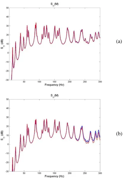
For studying the accuracy of the sampling method, one compares the previous result (dash 680

line) with the result of the sensitivity method (full line) on Fig. 8. A very good agreement between the two calculations can be observed. This indicates that although the panel response of the 30 realizations exhibits an important dispersion, an average over only 30 realizations is sufficient to give a correct estimation of the ASD function of the panel acceleration.

29 685

Fig. 8. 10log₁₀



S_

 

M



in function of frequency (dB, ref. 1 m/s2/Hz0.5). Comparison between three calculations: full line, the sensitivity function method (used as reference); dash line: the

sampling method with the modal forces calculated analytically; dashed-dotted line, the sampling method with the modal forces estimated using the fine mesh (25 x 9). Calculation

parameters: Corcos model, cutoff wavenumber criterion (34) based on the TBL 690

characteristics.

For this first result of the sampling method, Eq. (17) were used to synthetize the WPF and the modal forces were calculated analytically with Eq. (30). This is appropriate for academic cases. For more complex cases, the WPF will be defined on a point mesh and it will be 695

introduced in the numerical model of the panel. In the literature, different authors considering different spatial methods ([24], [25], [28]) already showed that the mesh of a finite element model should be defined carefully in this case for describing both, the structure behavior and the aerodynamic field. For studying the influence of the definition of the WPF on a discretized mesh in the framework of the proposed approach, let us considered a first mesh of points on the 700

plate. This will be called the fine mesh and it is defined by the spatial resolutions  and yx  defined by (as proposed in Ref. [25]):

    y x k y k x    and 2 , (37)

30 For the nominal test case, the mesh is composed of 25 points in the streamwise direction and 9 points in the crosswise direction. The modal forces used to estimate the plate acceleration 705

(29) can then be approximated using Eq. (31). The result of the sampling method considering the modal forces estimated on the fine mesh has been plotted (dashed-dotted line) on Fig. 8. One can observe that the discretization of the WPF using this fine mesh does not introduce significant discrepancy which is consistent with the works proposed in the literature.

710

4. Influence of the cut-off wavenumber criterion and the mesh size

Now, the accuracy of the sampling method is studied in function of the cut-off wavenumber criterion and the mesh size. To do that, a second mesh called the coarse mesh is considered with the spatial resolution in the streamwise direction defined by:

715 , 1   x k x   . (38)

where k is defined by the criterion (33). _x1

For the nominal test case, this coarse mesh is composed of 14 points in the streamwise direction. The spatial resolution in the crosswise direction remains unchanged compared to the fine mesh.

720

Results of the sampling method are compared to the sensitivity method on Fig. 9 when considering the coarse mesh and the two cutoff wavenumber criteria (33) and (34). Fig. 9a corresponds to the Corcos model whereas as Fig. 9b corresponds to the Chase model.

When the cut-off wavenumber criterion (34) based on the convective wavenumber is 725

considered, one notices that the discrepancies are generally less than 2 dB when the fine mesh is considered, whereas large discrepancies above around 180 Hz can be observed when the coarse mesh is used. This is observed for the two WPF models. Although the contributions of the convective ridge are filtered by the panel and may be neglected as shown in section V.C, a fine description of them is required in order to obtain good convergence of the calculation. In 730

contrary, when considering the coarse mesh and the cut-off wavenumber criterion (33) based on the flexural wavenumber, a good accuracy is observed on the whole frequency of interest, for both WPF models. This result confirm that the effect of the convective ridge is negligible on the panel vibration for the present case. Moreover, the coarse mesh is sufficient for

31 estimating the panel response because the pressure field of each realization (as shown on Fig. 735

5b) varies slowly when the criterion (33) is considered (contrary to the rapid variations of the pressure field when the criterion (34) is considered, as shown in Fig. 5a). This explains why the results converge with a coarse mesh when the criterion (33) is considered rather than the criterion (34).

(a)

(b)

Fig 9. 10log₁₀



S_

 

M



in function of frequency (dB, ref. 1 m/s2/Hz0.5). Results with two 740

different models of WPF: (a), Corcos; (b), Chase. Full line, the sensitivity function method (used as reference); dash line, the sampling method considering the coarse mesh (14 x 9) and

the cutoff wavenumber criterion (34) based on the TBL characteristics; dashed-dotted line: the sampling method considering the coarse mesh (14 x 9) and the cutoff wavenumber

criterion (33) based on the plate characteristics. 745