Benchmark for Algorithms Segmenting the Left Atrium From 3D CT and MRI Datasets

(1)

HAL Id: hal-01260607

https://hal-univ-rennes1.archives-ouvertes.fr/hal-01260607

Submitted on 31 Aug 2020

HAL is a multi-disciplinary open access

archive for the deposit and dissemination of

sci-entific research documents, whether they are

pub-lished or not. The documents may come from

teaching and research institutions in France or

abroad, or from public or private research centers.

L’archive ouverte pluridisciplinaire HAL, est

destinée au dépôt et à la diffusion de documents

scientifiques de niveau recherche, publiés ou non,

émanant des établissements d’enseignement et de

recherche français ou étrangers, des laboratoires

publics ou privés.

Benchmark for Algorithms Segmenting the Left Atrium

From 3D CT and MRI Datasets

Catalina Tobon-Gomez, Arjan Geers, Jochen Peters, Jürgen Weese, Karen

Pinto, Rashed Karim, Mohammed Ammar, Abdelaziz Daoudi, Jan Margeta,

Zulma Sandoval, et al.

To cite this version:

Catalina Tobon-Gomez, Arjan Geers, Jochen Peters, Jürgen Weese, Karen Pinto, et al.. Benchmark

for Algorithms Segmenting the Left Atrium From 3D CT and MRI Datasets. IEEE Transactions

on Medical Imaging, Institute of Electrical and Electronics Engineers, 2015, 34 (7), pp.1460–1473.

�10.1109/TMI.2015.2398818�. �hal-01260607�

(2)

This article has been accepted for publication in a future issue of this journal, but has not been fully edited. Content may change prior to final publication. Citation information: DOI 10.1109/TMI.2015.2398818, IEEE Transactions on Medical Imaging

1

Benchmark for algorithms segmenting the left

atrium from 3D CT and MRI datasets

Catalina Tobon-Gomez, Arjan J. Geers, Jochen Peters, J¨urgen Weese, Karen Pinto, Rashed Karim, Mohammed

Ammar, Abdelaziz Daoudi, Jan Margeta, Zulma Sandoval, Birgit Stender, Yefeng Zheng, Maria A. Zuluaga,

Julian Betancur, Nicholas Ayache, Mohammed Amine Chikh, Jean-Louis Dillenseger, B. Michael Kelm, Sa¨ıd

Mahmoudi, S´ebastien Ourselin, Alexander Schlaefer, Tobias Schaeffter, Reza Razavi, Kawal S. Rhode

Abstract—Knowledge of left atrial (LA) anatomy is important for atrial fibrillation ablation guidance, fibrosis quantification and biophysical modelling. Segmentation of the LA from Magnetic Resonance Imaging (MRI) and Computed Tomography (CT) images is a complex problem. This manuscript presents a benchmark to evaluate algorithms that address LA segmentation. The datasets, ground truth and evaluation code have been made publicly available through the http://www.cardiacatlas.org website. This manuscript also reports the results of the Left Atrial Segmentation Challenge (LASC) carried out at the STACOM’13 workshop, in conjunction with MICCAI’13. Thirty CT and 30 MRI datasets were provided to participants for segmentation. Each participant segmented the LA including a short part of the LA appendage trunk and proximal sections of the pulmonary veins (PVs). We present results for nine algorithms for CT and eight algorithms for MRI. Results showed that methodologies combining statistical models with region growing approaches were the most appropriate to handle the proposed task.

The ground truth and automatic segmentations were standard-C. Tobon-Gomez, K. Pinto, R. Karim, T. Schaeffter and K. S. Rhode are with Division of Imaging Sciences & Biomedical Engineering, King’s College London, London, United Kingdom. — A.J. Geers is with Universitat Pompeu Fabra, Barcelona, Spain. — J. Peters and J. Weese are with Philips GmbH Innovative Technologies, Research Laboratories, Hamburg, Germany. — M. Ammar and M. A. Chikh are with Biomedical Engineering Laboratory, University of Tlemcen, Tlemcen, Algeria. — A. Daoudi is with University of Bechar, Bechar, Algeria. — J. Margeta and N. Ayache are with Asclepios Re-search Project, INRIA Sophia-Antipolis, France. — Z. Sandoval, J. Betancur and J. L. Dillenseger are with Inserm, U1099, Rennes, F-35000, France; Université de Rennes 1, LTSI, Rennes, F-35000, France. — B. Stender is with Medical Robotics at Institute for Robotics and Cognitive Systems, University of Lübeck, Germany. — Y. Zheng and B. M. Kelm are with Siemens Corporate Technology in Princeton, NJ, USA and Erlangen, Germany, respectively. — M. A. Zuluaga and S. Ourselin are with the Translational Imaging Group, Centre for Medical Image Computing, University College London, London, United Kingdom. — S. Mahmoudi is with Computer Science Department, Faculty of Engineering, University of Mons, Mons, Belgium. — A. Schlaefer is with Medical Robotics at Institute for Robotics and Cognitive Systems, University of Lübeck, Germany; Institute of Medical Technology, Hamburg University of Technology, Hamburg, Germany.— R. Razavi is with Division of Imaging Sciences & Biomedical Engineering, King’s College London, London, UK and Department of Cardiology, Guy’s and St. Thomas’ NHS Foundation Trust, London, United Kingdom.

This research was supported by the National Institute for Health Re-search (NIHR) Guy’s and St Thomas’ Biomedical ReRe-search Centre, and, the NIHR University College London Hospitals Biomedical Research Centre (NIHR BRC UCLH/UCL High Impact Initiative-BW.mn.BRC10269). The views expressed are those of the author(s) and not necessarily those of the NHS, the NIHR or the Department of Health. This research was also supported by the German BMBF grant (01EZ1140A), the British EPSRC grant (EP/H046410/1), the French CardioUSgHIFU grant (ANR-2011-TecSan-004), the Microsoft Research PhD scholarship programme and the ERC advanced grant MedYMA.

Copyright (c) 2015 IEEE. Personal use of this material is permitted. However, permission to use this material for any other purposes must be obtained from the IEEE by sending a request to [email protected].

ised to reduce the influence of inconsistently defined regions (e. g. mitral plane, PVs end points, LA appendage). This standardisa-tion framework, which is a contribustandardisa-tion of this work, can be used to label and further analyse anatomical regions of the LA. By performing the standardisation directly on the left atrial surface, we can process multiple input data, including meshes exported from different electroanatomical mapping systems.

I. INTRODUCTION

A. Clinical motivation

Atrial fibrillation (AF) is the most common cardiac cal disorder [1]. Ablation therapies attempt to disrupt electri-cal reentry pathways that cause the arrhythmia. It has been shown that ectopic beats from within the pulmonary veins (PVs) commonly initiate AF [2]. The most common ablation procedure aims to electrically isolate the PVs from the left atrium (LA) body by inducing circumferential lesions. Some patients may require other types of lesions, such as linear lesions (e. g. along the roof or the isthmus), or complex localised lesions (e. g. targeting the autonomic ganglionated plexi) [1]. Traditionally, the ablation procedure has been guided with X-ray fluoroscopy. With the advances of clinical imaging systems, a preoperative CT or MRI scan is prescribed for most patients. This allows one to obtain a preoperative anatomical representation of the LA. This LA anatomy can be integrated into electroanatomical mapping systems. Such integration reduces fluoroscopy time and improves patient outcome [1]. A correct anatomical representation of the LA is, therefore, crucial for the success of the intervention.

Apart from therapy guidance, LA segmentations can help automate LA fibrosis quantification from late gadolinium enhancement datasets. The presence of LA fibrosis is highly associated with post-ablation AF recurrence [3]. Additionally, LA anatomical models have been employed for cardiac bio-physical modelling [4]. These models aim at understanding the mechanisms of AF and, eventually, at predicting optimal therapy.

B. Technical motivation

Segmentation is required to extract the LA anatomy from the preoperative scans. Segmenting the LA is challenging due to several reasons. The LA has a very thin myocardial wall (⇠2-3 mm) [5] making it challenging to image at even the best resolutions available. As a result, most algorithms

(3)

2 rely on extracting the blood pool to segment the LA which

leads to another complication. The LA is surrounded by other anatomical structures that appear with similar image intensity as the blood pool. These structures, including other cardiac chambers, the descending aorta and the coronary sinus, often mislead purely image driven algorithms. Additionally, the PV arrangement varies greatly between subjects. The topological variants include four veins (⇠74%), five veins (⇠17%) or three veins (⇠9%) [5]. The LA appendage (LAA) also varies in shape and size between subjects. Such anatomical variations limit the use of approaches with full statistical constraints. Finally, the mitral valve (MV) leaflets can be either at different opening positions or barely visible in the images. This hampers the definition of the boundary between the LA and the left ventricle.

Several approaches have been proposed to segment the LA from CT and/or MRI datasets. They have evolved from purely data driven methods, like region growing [6] or graph cuts [7], to more advanced methods using prior information. Prior information has mostly been included as an image atlas or a shape atlas. Zhuang et al. [8] used local affine and deformable registration to propagate a single atlas to an unseen image. This approach was extended to include multiple atlases which are fused to obtain a final segmentation [9]. Ecabert et al. [10] used a whole heart shape model trained with advanced image features [11]. This approach was extended to include multiple shape models with different PV topologies [12]. Zheng et al. [13] used a shape model approach which is automatically initialised using marginal space learning. Recent approaches tend to combine model based methodologies with image driven methodologies [14]–[17].

C. Benchmark and challenge

This manuscript presents a benchmark to evaluate algo-rithms that address LA segmentation. Benchmarking of al-gorithms is a very important activity to encourage clinical translation of image processing methods. It allows one to evaluate the algorithms using a unified database by an unbiased evaluator. In the last few years, several conferences have endorsed such benchmarks in the context of challenges. This manuscript also reports the results of the Left Atrial Seg-mentation Challenge (LASC) carried out at the STACOM’13 workshop, in conjunction with MICCAI’13 [18]. A second call for participants was issued after the workshop to ex-pand the range of evaluated algorithms. Consequently, this manuscript presents segmentation results from seven research groups covering a wide range of methodologies: thresholding with shape descriptors, statistical shape models with/without region growing, multi-atlas segmentation with/without region growing, snakes with region growing, and random decision forests. For further details, see Sec. III-B.

Performing an unbiased evaluation of different LA segmen-tation algorithms is a challenging task. Even for a human observer, it is difficult to define regions of the LA, such as the MV plane, the PVs and the LAA. To ensure that the calculated metrics are not negatively affected by inconsistent definitions of these regions, we developed a standardisation

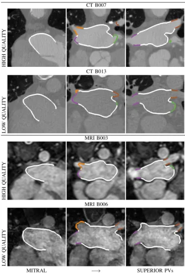
CT B007 HIGH Q U ALITY CT B013 LO W Q U ALITY MRI B003 HIGH Q U ALITY MRI B006 LO W Q U ALITY MITRAL SUPERIOR PVs

HEART DETECTION SIMILARITY TRANSFORM PIECEWISE AFFINE DEFORMABLE

a b c d

MV PLANE CENTRELINES DIAMETER_CHANGE PV LABELS

SUPERIOR

a b c d

VORONOI _VORONOISMOOTH LAA LABEL CLIPPING

SUPERIOR

e f g h

Fig. 1: Examples of datasets provided for the benchmark. A high and a low quality dataset is displayed for each modality. Colour contours show the manual ground truth (LA body = white, LAA = green, PVs = other colours). For more details see Sec. II-A.

framework. First, we extract a 3D mesh from the binary masks. We then compute the MV plane and use it to truncate the meshes. Subsequently, we automatically find the PV ostia and label the PVs accordingly. We use these automatic labels1 _to truncate the PVs distally to the LA body ensuring at least 10 mm coverage. Finally, the LAA is labelled and discarded from metric computation. The standardisation framework was executed both on the ground truth and the automatically segmented binary masks. This framework is an important part of the contribution of this work and can be used to label and further analyse anatomical regions of the LA. For further details, see Sec. II.

II. EVALUATION FRAMEWORK

A. Datasets

Thirty CT and 30 MRI datasets were provided to par-ticipants for segmentation. Ten data sets per modality were provided with expert manual segmentations for algorithm training (SET-A). The other 20 data sets per modality were

1_{Labels are commonly used in image processing to identify different regions}

in a segmented mask. By displaying each label with a different colour, each region is easily visually identified.

(4)

3 used for evaluation (SET-B). Datasets were limited to the

most common topological variants showing four PVs (present in ⇠74% of the population). The datasets were provided by Philips Technologie GmbH, Hamburg, DE, and King’s College London, London, UK (see Fig. 1).

1) CT datasets: Retrospectively ECG-gated cardiac multi-slice CT images were acquired with Philips 16-, 40-, 64- and 256-slice scanners (Brilliance CT and Brilliance iCT, Philips Healthcare, Cleveland OH, USA) typically at end-systole. All images were reconstructed using a 512 ⇥ 512 matrix with an in-plane voxel resolution ranging from 0.30 ⇥ 0.30 to 0.78 ⇥

0.78mm2 _{and with a slice thickness ranging from 0.33 to}

1.00 mm. All scans were acquired after injection of ca. 40– 100 ml contrast media. Acquisition times for a complete CT volume ranged from 4 s on modern iCT scanners to 20 s for the older 16-slice scanners. Each dataset represents a single cardiac phase 3D volume image. The datasets were selected to provide a variety of quality levels in the following proportions: 8 high contrast, 15 moderate contrast, 3 low contrast and 4 high noise datasets.

2) MRI datasets: MRI acquisition was performed on a 1.5 T Achieva scanner (Philips Healthcare, Best, The Nether-lands). A 3D whole heart image was acquired using a 3D balanced steady state free precession acquisition [19]. The sequence acquired a non-angulated volume covering the whole heart with voxel resolution of 1.25 ⇥ 1.25 ⇥ 2.7 mm3_{. Images} were acquired during free breathing with respiratory gating and at end diastole with ECG gating. Typical acquisition time for a complete volume was 10 min. Each dataset represents a single cardiac phase 3D volume image. The datasets were selected to provide a variety of quality levels in the following proportions: 9 high quality, 10 moderate quality, 6 local artefacts and 5 high noise datasets.

B. Ground truth generation

In order to obtain a set of ground truth (GT) segmentations consistent across modalities, we started by performing an automatic model based segmentation with a method which is optimised for both CT and MRI modalities. After the automatic segmentation, manual corrections were performed. This algorithm was not included in the evaluation to avoid statistical bias. Details are provided next.

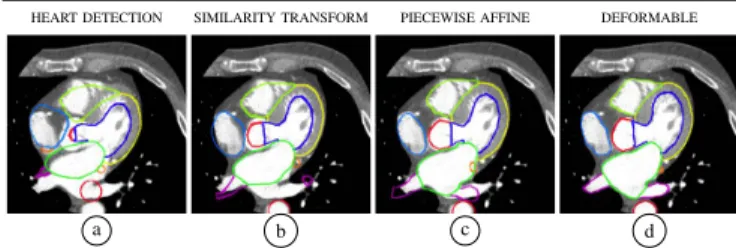
1) Automatic segmentation: The automatic segmentation used in this study was described in [10], [20], [21]. The seg-mentation uses shape constrained deformable models. These are based on a mesh representation of surfaces of cardiac chambers and the attached great vessels. The automatic adapta-tion starts by a localisaadapta-tion step using the Generalised Hough Transform [22] to place the mesh model close to the heart (Fig. 2-a). Several adaptation steps with increasing degrees of freedom refine the model’s pose and shape. Each step uses trained boundary detectors to detect each chamber’s boundaries in the image. Using the detected boundaries, a first step adjusts the global pose of the complete model by performing a rigid adaptation with scaling that minimises the squared distances of the model surface to the detected boundaries (Fig. 2-b). Subsequent steps add more degrees of

a b c d

SUPERIOR

a b c d

SUPERIOR

e f g h

Fig. 2: Automatic segmentation pipeline on a CT image for ground truth generation. Different colours represent different parts of the deformable model. Green and magenta regions correspond to the LA and the PVs, respectively (for details see Sec. II-B1).

freedom by subdividing the model into mesh regions and adapts these parts via individual affine transformations (Fig. 2-c). Finally, a deformable adaptation step leads to a locally accurate segmentation in which each mesh vertex is free to move under the image forces that pull the mesh triangles to the detected boundaries while internal forces regularise the adaptation and penalise strong deformations of the model shape (Fig. 2-d). After adaptation of the model is complete, the regions enclosed by the surfaces are converted into a label image with region-specific labels. In our study, labels not covering the LA and the PVs were discarded.

2) Manual correction criteria: Each automatic segmenta-tion was manually corrected by an experienced observer to obtain the final GT segmentation. Additionally, a second ob-server (OBS-2) performed the manual corrections to estimate interobserver variability. Manual corrections were performed using Philips in-house editing tools and/or ITK-SNAP [23]. PVs were followed distally to the LA body ensuring at least 10 mm coverage. They were truncated at the first branching point when there was no clear main PV to follow. Editing was performed on all orthogonal slices. Observers also itera-tively generated isosurfaces of the segmentation to ensure 3D consistency and to remove surface irregularities. The amount of time dedicated to a dataset ranged between 2 and 6 hours. Each GT segmentation consisted of five labels: one label for the LA body including the LAA and one label for each of the four PVs. The LAA was truncated relatively close to the body to ease GT generation. These labels were used only for standardisation purposes (see Sec. II-C1).

C. Standardisation

Even for a human observer, it is difficult to define regions of the LA, such as the MV plane, the PVs and the LAA. To ensure that the calculated metrics are not negatively affected by inconsistent definitions of these regions, we standardised all the manual GT and all submitted segmentations. The framework was implemented using the Visualization Toolkit

(VTK),2 _{the Vascular Modeling Toolkit (VMTK),}3 _and

MAT-LAB Toolbox graph.4

1) Mitral valve plane: The boundary between the atrium and the ventricle can be inconsistent due to different levels or opening/closure of the MV leaflets. To compute the mitral plane, we generate a surface mesh from the GT label images

2_www.vtk.org 3_www.vmtk.org

(5)

4 using marching cubes followed by volume preserving

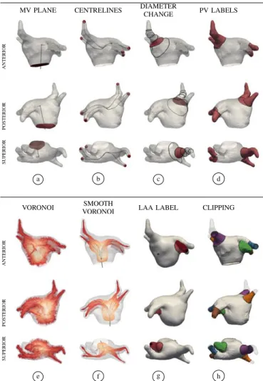
smooth-ing. We define a local coordinate system using the centroid of the LA body (BC) and the centroid of the four PV ostia (PVC). The first axis is the vector connecting the BC and the PVC. The second axis is computed perpendicularly to the first axis and the vector connecting left and right PVC. The third axis is computed perpendicularly to the first and second axes. These three axes are combined using empirically determined weights. The clipping plane is set normal to the combined vector and centred at a point below the BC. Segmentations are truncated below the MV plane (Fig. 3-a). We verified the accuracy of this clipping approach in the original images.

2) Pulmonary veins ostia: Due to a lack of clear anatomical landmarks, defining the boundary between the LA body and each PV is not trivial (i. e. ostia). In this study, we developed an automatic approach to obtain a consistent and 3D sound definition of the PV ostia. This approach makes use of a Voronoi diagram extracted from the surface mesh and its corresponding centrelines [24]. To extract the source and target seeds for centreline construction, we compute the Gauss curvature on the surface [25], [26]. For each PV we select the high curvature patch furthest from the body and store its centroid as a PV seed. From the patches belonging to the body, we keep the largest patch and store its centroid as a LAA seed (red spheres in Fig. 3-b).

For each PV, we generate a pair of centrelines that connect the PV seed to the two opposite PV seeds, as displayed in Fig. 3-b. We split the centrelines into branches [27] and create cross sections perpendicular to the centreline. As the clipping section enters the LA body, the maximum diameter increases significantly, providing the ostium point (Fig. 3-c). We clip the surface at the ostium point and use the isolated PV to relabel the original surface (Fig. 3-d).

3) Left atrial appendage: The great variation of the LAA in the population makes it difficult to segment. To label the LAA, we reconstruct a simplified version of the original surface based on a smooth Voronoi diagram (Fig. 3-e) [28]. We then compute the distance between the original and the simplified reconstructed surface (Fig. 3-f). We evaluate large distance patches as candidate LAA regions. We select the patch closest to the previously computed LAA seed (Fig. 3-g).

4) Pulmonary vein truncation: For this benchmark, we wish to retain only the proximal sections of each vein. Truncation is performed by clipping the PV with a plane perpendicular to its corresponding centreline (Fig. 3-h). The clipping point is computed by measuring 10 mm from the ostium along the centreline.

D. Evaluation metrics

To test segmentation accuracy we used two metrics: surface-to-surface distance (S2S) and Dice coefficient (DC). S2S gives the distance in mm of each point in the automatically seg-mented mesh to the GT surface. Low values of S2S represent higher accuracy. We computed S2S between each standardised GT mesh and each standardised automatic mesh, and vice versa. To normalise the contribution of each case to the average S2S metric, distance measurements were subsampled

a b c d

SUPERIOR

a b c d

SUPERIOR

e f g h

Fig. 3: Standardisation framework. A surface mesh is computed from the GT label images. The mesh is clipped at the MV plane. The centroids of the high curvature areas are used as seed points for centreline extraction. The ostium of each PV is automatically defined based on the change of diameter (fewer diameter sections are displayed). New labels are assigned to the mesh representing each PV. To label the LAA, the Voronoi diagram is smoothed along the centrelines and a simplified surface is reconstructed. By computing the distance from the original surface to the simplified surface, we extract the LAA region. Each PV is isolated and clipped with a plane perpendicular to the centreline and located 10 mm away from the ostia (for details see Sec. II-C). to 2000 random samples (per case and per region) using a bootstrapping approach.

DC summarises volumetric overlap between two sets of binary segmentations. Values of 0 indicate no overlap between the result and the GT. Values of 1 indicate complete overlap (higher accuracy). To calculate the DC, we generated a blank image with the same resolution as the input datasets. We then isolated each region from the standardised meshes and marked the voxels inside the surface with its corresponding GT label value. We computed the overlap between the new GT label images and the automatic images.

In our experience, S2S best reflects segmentation accuracy for the LA body, while DC best reflects segmentation ac-curacy for the PVs. We combined these two metrics into a unified score representing relative deviation from the mean. To equalise the contribution of both metrics, we normalised each error measurement such that:

Zreg,p=

xp µ

(6)

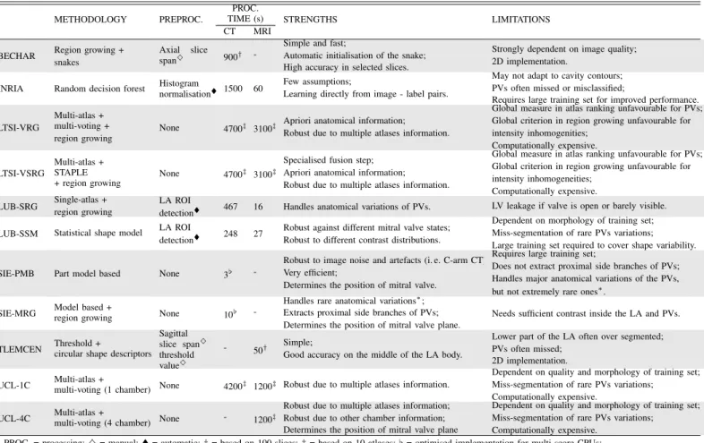
5 TABLE I: Summary of algorithms evaluated in this benchmark.

METHODOLOGY PREPROC. TIME (s)PROC. STRENGTHS LIMITATIONS

CT MRI

BECHAR Region growing +_snakes Axial slice_span} 900†

-Simple and fast;

Automatic initialisation of the snake; High accuracy in selected slices.

Strongly dependent on image quality; 2D implementation.

INRIA Random decision forest Histogram_{normalisation}⌥ 1500 60 Few assumptions;_{Learning directly from image - label pairs.}

May not adapt to cavity contours; PVs often missed or misclassified;

Requires large training set for improved performance. LTSI-VRG

Multi-atlas + multi-voting +

region growing None 4700

‡ ₃₁₀₀‡ Apriori anatomical information;

Robust due to multiple atlases information.

Global measure in atlas ranking unfavourable for PVs; Global criterion in region growing unfavourable for intensity inhomogenities;

Computationally expensive. LTSI-VSRG Multi-atlas +STAPLE

+ region growing None 4700

‡ ₃₁₀₀‡

Specialised fusion step; Apriori anatomical information; Robust due to multiple atlases information.

Global measure in atlas ranking unfavourable for PVs; Global criterion in region growing unfavourable for intensity inhomogeneities;

Computationally expensive.

LUB-SRG Single-atlas +_{region growing} LA ROI_detection⌥ 467 16 Handles anatomical variations of PVs. LV leakage if valve is open or barely visible.

LUB-SSM Statistical shape model LA ROI

detection⌥ 248 27 Robust against different mitral valve states;_{Robust to different contrast distributions.}

Dependent on morphology of training set; Miss-segmentation of rare PVs variations; Large training set required to cover shape variability.

SIE-PMB Part model based None 3[

-Robust to image noise and artefacts (i. e. C-arm CT); Very efficient;

Determines the position of mitral valve.

Requires large training set;

Does not extract proximal side branches of PVs; Handles major anatomical variations of the PVs, but not extremely rare ones⇤_.

SIE-MRG Model based +_{region growing} None 10[

-Handles rare anatomical variations⇤_;

Extracts proximal side branches of PVs;

Determines the position of mitral valve plane. Needs sufficient contrast inside the LA and PVs. TLEMCEN Threshold +_{circular shape descriptors}

Sagittal slice span}

threshold value}

- ₅₀† Simple;

Good accuracy on the middle of the LA body.

Lower part of the LA often over segmented; PVs often missed;

2D implementation. UCL-1C Multi-atlas +_{multi-voting (1 chamber) None} 4200‡ ₁₂₀₀‡ _{Robust due to multiple atlases information.}

Dependent on quality and morphology of training set; Miss-segmentation of rare PVs variations;

Computationally expensive. UCL-4C Multi-atlas +_{multi-voting (4 chamber) None} - ₁₂₀₀‡

Robust due to multiple atlases information; Robust due to other chamber information; Determines the position of mitral valve plane

Dependent on quality and morphology of training set; Miss-segmentation of rare PVs variations;

Computationally expensive. PROC. = processing; } = manual; ⌥ = automatic; † = based on 100 slices; ‡ = based on 10 atlases; [ = optimised implementation for multi-score CPUs; ⇤ = not included in this benchmark; Processing times not directly comparable due to different types of CPUs.

where reg is the anatomical region (body, PVs), xp is the median metric of each participant (p), µ is the mean of the median metric of all participants, and, is the standard deviation of the median metric of all participants. We used the complement of the DC (1-DC) previous to normalisation so that, similarly to S2S, lower values translate into higher accuracy.

After normalisation, the unified score Spfor each participant

pwas computed as:

Sp=

ZS2Sbody,p+ Z(1 DC)pvs,p

2 (2)

III. CHALLENGE RESULTS

To simplify the segmentation task, participants were pro-vided with a single value mask combining all structures for training. They were asked to segment the LA including a short part of the LAA and the proximal sections of the PVs as a single-valued mask. The LA body should have reached into the funnel of the MV. To encourage submissions with more incipient segmentation techniques, we stated in the call that errors corresponding to the LAA would be excluded. Since the standardisation procedure was stated upon data request, participants were aware that evaluation metrics would not punish long PVs or LV leakage.

A. Automatic segmentations

From each binary mask we generated a surface mesh using marching cubes followed by volume preserving smoothing (to correct marching cubes artefacts). Next, we clipped the mesh with the MV plane generated from the GT mesh (Sec. II-C1), discarding unconnected regions. We then transferred the au-tomatic PVs and LAA labels of the GT mesh to their closest points in the automatically segmented mesh (Sec. II-C2 and Sec. II-C3). For each label, we ensured a single connected region to avoid transferring PV labels to neighbouring areas. Finally, using the automatic labels, we clipped the PVs using the planes computed automatically from the GT (Sec. II-C4). B. Evaluated algorithms

We received 11 submissions from seven international groups. Table I details the characteristics of each algorithm. Due to the use of different types of CPUs for execution, we could not directly compare the execution time of the different algorithms. We provide below a brief description of their underlying methodology. Note that all operations were performed in 3D unless stated otherwise.

a) University of Bechar, Algeria (BECHAR): Daoudi et al. [29] proposed an algorithm based on active contours. It started by enhancing image contrast using an adaptive histogram equalisation method. Each image (SET-B) was then thresholded to roughly localise a seed point inside the LA. The region around the seed point was

(7)

6 gradually grown to produce a preliminary segmentation. This

preliminary segmentation was used to initialise a Gradient Vector Flow snake model which was attracted to the borders of the LA. This is a 2D approach and requires a preselection of the axial slices spanning the LA. Only CT datasets were processed.

b) Inria, Sophia-Antipolis, France (INRIA):

Margeta et al. [30] proposed an algorithm based on random decision forests. The algorithm had an offline training phase in which binary decision trees were optimised to separate the atrial voxels from the background voxels (SET-A). The decision trees used several features such as: local intensity, long-range intensity relationship, distance to blood pool contours and tubularity. During the online segmentation phase (SET-B), each voxel was assigned a probability of belonging to the LA based on these trees. The final segmentation was obtained by thresholding the probability map. Postprocessing included a hole filling step and extraction of the largest connected component. Both modalities were processed.

c) LTSI - Inserm Rennes, France (LTSI): Sandoval et al. [16] proposed one algorithm based on multi-atlas segmentation followed by region growing. It started by performing affine registration between the unseen image (SET-B) and each atlas intensity image (SET-A). A subset of top-ranked atlas intensity images were selected according to the final similarity measure value. The subset were registered to the unseen image using elastic registration. The obtained transformations were used to propagate the atlas label images to the unseen image space. The propagated atlas labels were merged using fusion rules. Finally, this fused label image was eroded and used to initialise a region growing procedure. The same fused label image was dilated to spatially constrain the region growing. Both modalities were processed using two different fusion rules: majority-voting (LTSI-VRG) and STAPLE (LTSI-VSRG).

d) University of L¨ubeck, Germany (LUB): Stender et al. [15] proposed two algorithms. The first algorithm was based on statistical shape models (LUB-SSM). This algorithm used an average image constructed from SET-A which was used to construct a modality-specific statistical shape model. To initialise the segmentation, the unseen image (SET-B) was registered to the average image using affine registration. The obtained transformation was used to propagate the average mesh. The mesh was subsequently adapted along the surface normals of each vertex following gradient features of the unseen image. A valid instance of the deformed mesh was obtained using the statistical constraints of the model. Both modalities were processed.

The second algorithm was based on statistical region grow-ing (LUB-SRG). In this algorithm the unseen image (SET-B) was registered to the average image using affine and elastic registration. The voxels with high probability of being inside the LA were used as seed points for the region growing procedure. The final segmentation was obtained after a hole filling procedure. Both modalities were processed.

e) Siemens Corporate Technology, Princeton, NJ, USA (SIE): Zheng et al. [13], [17] proposed two algorithms. The first algorithm was based on a multi-part model (SIE-PMB) divided into six-parts: LA body, LAA and four PVs. Each part

was detected and segmented using marginal space learning. To improve detection robustness, statistical shape constraints were enforced during marginal space learning pose estimation. Finally, all parts were merged into a consolidated mesh. The algorithm was previously trained on 457 cardiac CT scans. Only CT datasets were processed.

The second algorithm was based on shape models followed by region growing (SIE-MRG). In this approach the LA body and LAA were segmented using marginal space learning. The PVs were segmented using region growing. Based on the LA body segmentation, the parameters for region growing were adaptively determined for each volume. Finally, graph cuts postprocessing was used to remove leakage. For the graph cuts, the tissues outside the region growing segmentation were negative seeds and the LA body and LAA were positive seeds. The graph cuts were performed on a down-sampled volume to reduce computational cost. Only CT datasets were processed. f) University of Tlemcen, Algeria (TLEMCEN): Am-mar et al. [31] proposed an algorithm based on threshold localisation and circularity shape descriptors. This algorithm processed sagittal slices since on this view the LA appears ellipsoidal. Each slice was thresholded and each separate region was analysed for shape features, including: circularity, elongation, area, centre of mass. The optimal distinguishing features were trained from SET-A. This is a 2D approach and requires a preselection of the sagittal slices spanning the LA. Only MRI datasets were processed.

g) University College London, United Kingdom (UCL): Zuluaga et al. [9] proposed one algorithm based on multi-atlas segmentation propagation. In this algorithm, the unseen image (SET-B) was registered to each atlas intensity image using affine and elastic registration. The obtained transformations were used to propagate the atlas label images to the unseen image space. The propagated labels were fused using the STEPS algorithm [32]. The propagated atlas images were ranked based on Local Normalised Correlation Coefficient Criterion ranking strategy. Only the top-ranked atlas images were used to obtain the final segmentation. Both modalities were processed using SET-A as input atlas set (UCL-1C). MRI datasets were also processed using a four-chamber in-house atlas set (UCL-4C).

IV. RESULTS

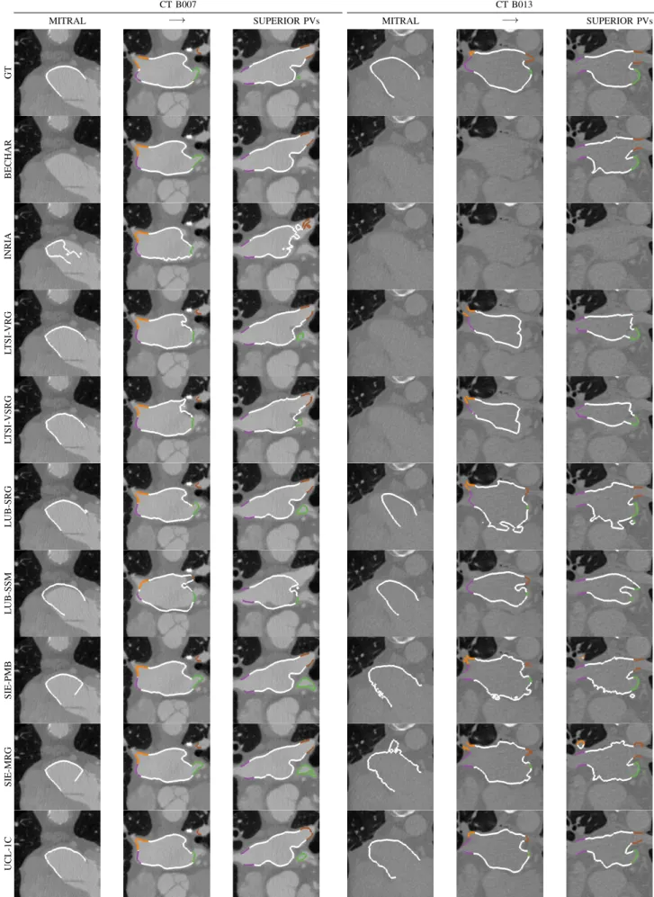
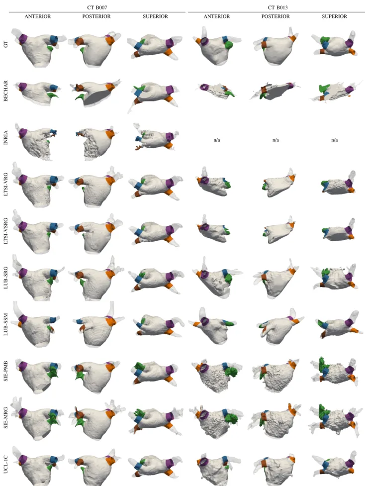
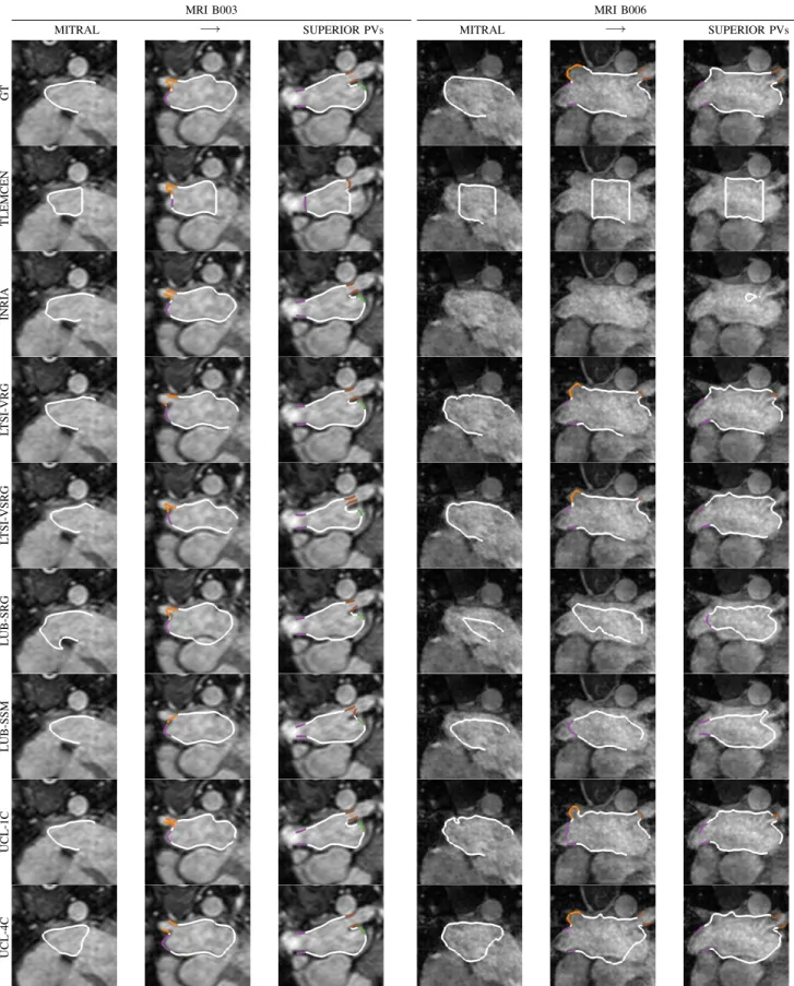
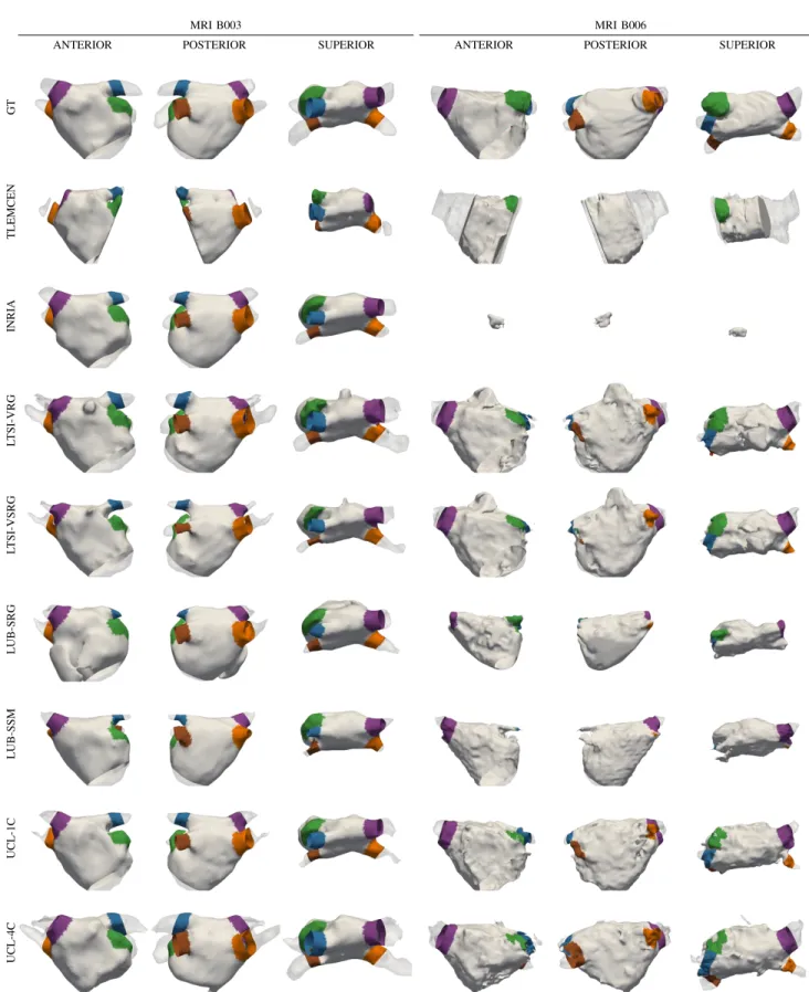
Visual results of the segmentation outputs are displayed for each algorithm and both modalities in Fig. 4 to Fig. 7. Fig. 4 and Fig. 6 show axial slices from CT and MRI datasets, respectively. The standardised meshes were intersected by the image plane to generate contours. Fig. 5 and Fig. 7 show a rendering of the output meshes from CT and MRI datasets, respectively. The original meshes are displayed with trans-parency, while the standardised meshes are opaque and colour mapped according to anatomical region. The GT is placed on the top row as reference. For each modality, we present a high quality and a low quality dataset. Additional figures are included as supplementary material.

(8)

7 2

CT B007 CT B013

MITRAL SUPERIOR PVs MITRAL SUPERIOR PVs

GT BECHAR INRIA LTSI-VRG LTSI-VSRG LUB-SRG LUB-SSM SIE-PMB SIE-MRG UCL-1C

Fig. 4: Axial slices from the CT datasets are displayed from the mitral to the PVs plane. The standardised meshes were intersected by the image plane to generate contours. They are colour mapped according to anatomical region (LA body = white, LAA = green, PVs = other colours). Case B007 is a high quality dataset. Common failures included joining of the left inferior PV with the LAA, and, leakage into the left ventricle, the aorta and/or the right atrium. Case B013 is a low quality dataset. For this case, region growing introduced irregularities on the final segmentation. Decision forest algorithm (INRIA) failed on this dataset.

(9)

8 3

CT B007 CT B013

ANTERIOR POSTERIOR SUPERIOR ANTERIOR POSTERIOR SUPERIOR

GT

BECHAR

INRIA n/a n/a n/a

LTSI-VRG LTSI-VSRG LUB-SRG LUB-SSM SIE-PMB SIE-MRG UCL-1C

Fig. 5: Results for each algorithm on the CT datasets. The original meshes are displayed with transparency. The standardised meshes are colour mapped according to anatomical region (for details see Sec. III-A). Case B007 is a high quality dataset. Common failures included joining of the left inferior PV with the LAA, and, leakage into the left ventricle, the aorta and/or the right atrium. Case B013 is a low quality dataset. For this case, region growing introduced irregularities on the final segmentation. Decision forest algorithm (INRIA) failed on this dataset.

(10)

9 4

MRI B003 MRI B006

MITRAL SUPERIOR PVs MITRAL SUPERIOR PVs

GT TLEMCEN INRIA LTSI-VRG LTSI-VSRG LUB-SRG LUB-SSM UCL-1C UCL-4C

Fig. 6: Axial slices from the MRI datasets are displayed from the mitral to the PVs plane. The standardised meshes were intersected by the image plane to generate contours. They are colour mapped according to anatomical region (LA body = white, LAA = green, PVs = other colours). Case B003 is a high quality dataset. Case B006 is a low quality dataset. For this case, region growing introduced irregularities on the final segmentation and decision forest retrieved a only few pixels inside the body.

(11)

10 5

MRI B003 MRI B006

ANTERIOR POSTERIOR SUPERIOR ANTERIOR POSTERIOR SUPERIOR

GT TLEMCEN INRIA LTSI-VRG LTSI-VSRG LUB-SRG LUB-SSM UCL-1C UCL-4C

Fig. 7: Results for each algorithm on the MRI datasets. The original meshes are displayed with transparency. The standardised meshes are colour mapped according to anatomical region (for details see Sec. III-A). Case B003 is a high quality dataset. Case B006 is a low quality dataset. For this case, region growing introduced irregularities on the final segmentation and decision forest retrieved a only few pixels inside the body.

(12)

11 CT DATASETS a SURFACE-TO-SURFACE DISTANCE (mm) 0 1 2 3 4 5 6 7 8 9 10 11 12 13 14 15

BECHAR INRIALTSI_VRGLTSI_VSRGLUB_SRGLUB_SSMSIE_PMBSIE_MRGTLEMCENUCL_1C UCL_4C OBS_2

0 1 2 3 4 5 6 7 8 9 10 11 12 13 14 15

b DICE COEFFICIENT (index)

0 0.1 0.2 0.3 0.4 0.5 0.6 0.7 0.8 0.9 1

BECHAR INRIALTSI_VRGLTSI_VSRGLUB_SRGLUB_SSMSIE_PMBSIE_MRGTLEMCENUCL_1C UCL_4COBS_2 MRI DATASETS c SURFACE-TO-SURFACE DISTANCE (mm) 0 1 2 3 4 5 6 7 8 9 10 11 12 13 14 15

BECHAR INRIALTSI_VRGLTSI_VSRGLUB_SRGLUB_SSMSIE_PMBSIE_MRGTLEMCENUCL_1C UCL_4C OBS_2 0 1 2 3 4 5 6 7 8 9 10 11 12 13 14 15

d DICE COEFFICIENT (index)

0 0.1 0.2 0.3 0.4 0.5 0.6 0.7 0.8 0.9 1

BECHAR INRIALTSI_VRGLTSI_VSRGLUB_SRGLUB_SSMSIE_PMBSIE_MRGTLEMCENUCL_1C UCL_4C OBS_2 0 0.1 0.2 0.3 0.4 0.5 0.6 0.7 0.8 0.9 1

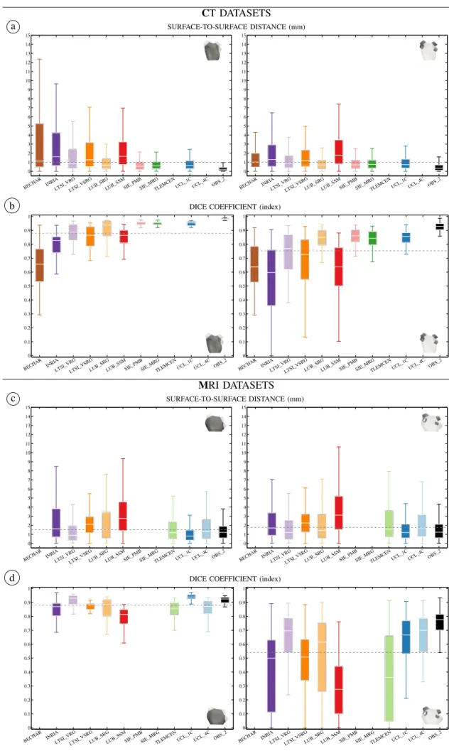
Fig. 8: Box plots of S2S (a+c) and DC (b+d) metrics for each algorithm. The corresponding region is represented with vignettes: LA body without LAA (left) and all four PVs (right). The dotted line represents the mean of the median metrics of all participants. Maximum whisker corresponds to ⇠99.3% coverage if the data were normally distributed.

(13)

12 The evaluation metrics were grouped in two sets of errors:

the LA body after LAA removal and the four PVs combined. Fig. 8-a and Fig. 8-c show the results of the surface-to-surface distances as box plots. Each box plot was computed from 40000 samples corresponding to 2000 samples per case. Fig. 8-b and Fig. 8-d show the results for the Dice coefficient as 8-box plots. Each box plot was computed from one value for the body and four values for the PVs per case. Errors corresponding to the LAA were not included in metric computation. The metrics corresponding to interobserver variability were also included in the plot. The median and standard deviation values for both metrics are summarised in tables attached as supplementary material.

Fig. 9 shows the unified scores computed using Eq. 1 and Eq. 2 for both modalities. Note that metrics corresponding to OBS-2 were not included in the normalisation. The normali-sation values used to compute CT scores were: µS2S = 0.99,

S2S = 0.44, µ(1 DC)= 0.27, (1 DC)= 0.11. The

normal-isation values used to compute MRI scores were: µS2S = 1.52,

S2S = 0.68, µ(1 DC)= 0.46, (1 DC)= 0.16.

V. DISCUSSION

A. Overview

Although each algorithm is different in underlying method-ology and implementation, we can find a few overall ten-dencies: (1) a preprocessing procedure such as histogram normalisation, volume of interest selection or atrial body lo-cation; (2) obtaining an initial segmentation using a statistical approach (multi-atlas or shape model); (3) optimisation of the segmentation using region growing or snakes (overall or limited to PV regions); (4) a post processing procedure such as hole filling to regularise the segmentation or graph cuts to reduce the leakage introduced by region growing.

To select a segmentation approach, one should take into account the characteristics of each algorithm (Table I) and the clinical context. For therapy guidance, either with elec-troanatomical fusion/merging or fluoroscopy overlay, the error induced by registration and respiratory motion alone is typi-cally 1-2 mm [33]. For patient follow-up, the goal is to have a segmentation that represents the LA anatomy to automate scar quantification in late gadolinium enhancement datasets. A common approach is to probe pixels around the LA border for presence of fibrosis. If the search is bounded to ±3 mm from the edge of the segmentation [34], a segmentation results <3 mm from the actual LA wall would retrieve similar scar information. For cardiac biophysical modelling, one could trade anatomical accuracy to obtain a smoother surface. B. CT datasets

Except in cases of poor image contrast, CT datasets allowed for a clear visualisation of the LA body and PVs. This is evident from the low interobserver variability (OBS-2). For this modality, statistical atlas/shape approaches with/without region growing obtained the best results. As can be seen in Fig. 9-a, these methods obtained above average accuracy (neg-ative scores): LTSI-VRG, LUB-SRG, SIE-PMB, SIE-MRG,

a CT DATASETS −2 −1.5 −1 −0.5 0 0.5 1 1.5 2 0.68 1.43 −0.22 0.43 −0.85 1.30 −1.01−0.89 −0.88 −1.73

BECHAR INRIALTSI_VRGLTSI_VSRGLUB_SRGLUB_SSMSIE_PMBSIE_MRGTLEMCENUCL_1CUCL_4C OBS_2

b MRI DATASETS −2 −1.5 −1 −0.5 0 0.5 1 1.5 2 0.20 −0.98 0.54 −0.24 1.79 0.30 −0.94 −0.67 −0.98

BECHAR INRIALTSI_VRGLTSI_VSRGLUB_SRGLUB_SSMSIE_PMBSIE_MRGTLEMCENUCL_1CUCL_4C OBS_2

Fig. 9: Unified scores computed using Eq. 1 and Eq. 2. The score combines the S2S distance for the LA body and the DC for the PVs (1-DC). Lower values represent higher accuracy. Zero represents the average accuracy of all evaluated methods. The black bar represents interobserver variability (OBS-2). UCL-1C. In low SNR images, region growing introduced ir-regularities on the final segmentation (see Fig. 5-B013). Other common failures included joining of the left inferior PV with the LAA, and, leakage into the left ventricle, the aorta and/or the right atrium. Left ventricular leakage was removed by our standardisation process, hence they were not penalised by the evaluation metrics. However, to be implemented as a feasible clinical tool, the region growing should be somewhat constrained. For instance, a postprocessing step using graph cuts (SIE-MRG) proved to successfully contain unwanted leakage into the right pulmonary artery after region growing. Alternatively, limiting the region growing process to the PV regions and/or to the surroundings of the initial segmentation could serve the same purpose.

As can be seen in Fig. 9-a, these methods obtained below average accuracy (positive scores): BECHAR, INRIA, LTSI-VSRG, LUB-SSM. BECHAR shows potential since the slices that were processed obtained good accuracy. Unfortunately, due to the large amount of missing slices (especially on the lower part of the LA body) the performance metrics were heavily punished. A 3D extension of the approach able

(14)

13 to handle the whole span of the LA would increase the

feasibility of the methodology. The generality of INRIA’s decision forests comes at the cost of rather large training sets, with typically several hundred subjects. The current disparity in error metrics may be due to the large variation of intensities and shapes across the given dataset with ten training subjects in each modality. Improvements could be expected with larger training sets. The method could also benefit from using specific shape constraints based on the LA anatomy. LTSI-VSRG obtained lower accuracy than its counterpart (LTSI-VRG) by introducing a different fusion rule. Both of these approaches (LTSI-VRG and LTSI-VSRG) can benefit from increasing the number of atlases and optimising the region growing parameters on a case-by-case fashion. LUB-SSM obtained valid shape instances of the LA due its statistical constraints. However, it obtained lower accuracy than its counterpart (LUB-SRG). In order to capture a large range of shape variability, the training set needs to be extensive (e. g. SIE-PMB was previously trained with 457 datasets). C. MRI datasets

MRI datasets proved more challenging to segment due to their lower spatial resolution and intensity inhomogeneities. This is evident on the higher interobserver variability (OBS-2). In fact, the task with lowest overall accuracy was PV segmen-tation from MRI datasets. In this sense, atlas based approaches are advantageous. As can be seen in Fig. 9-b, these methods obtained above average accuracy (negative scores): LTSI-VRG, LUB-SRG, UCL-1C, UCL-4C. We noticed increased inaccuracies on cases with a left common trunk. Ideally, these models should be trained with a large dataset including all anatomical variations. LTSI-VRG and LUB-SRG approaches behaved similarly than for CT datasets (see Sec. V-B). UCL-4C obtained lower accuracy than its counterpart (UCL-1C). This could be due to different labelling on the in-house atlas set.

As can be seen in Fig. 9-b, these methods obtained be-low average accuracy (positive scores): INRIA, LTSI-VSRG, LUB-SSM, TLEMCEN. INRIA often obtained good results despite its few methodological assumptions. However, when the segmentation failed the errors were rather large resulting in a large dispersion of error metrics. A possible improvement of this approach could be similar to CT, i. e. increase the size and variability of the training dataset, and, include shape constraints on the raw output of the forest. PV segmentation performance could be improved by using the complete label map (LA, PVs and background) and by increasing weights of the less represented PV voxels in the decision forest training. LTSI-VSRG and LUB-SSM approaches behaved similarly to the CT datasets (see Sec. V-B). TLEMCEN’s algorithm is based on circular shape descriptors from the sagittal plane. Thus, similar to more complex approaches, it obtained good accuracy on the middle of the LA body. However, the PVs were often missing and the lower part of the LA body (closer to the MV) was often over segmented. Similarly to BECHAR, a 3D extension could improve its feasibility for a clinical application.

D. Limitations and Future work

This benchmark includes a limited number of training cases (SET-A) representing ⇠74% of the PV anatomical variants. In this sense, more mature methodologies with previous training had an advantage over algorithms implemented specifically for this evaluation.

Generating a GT is a non-trivial task for which one needs to balance control vs. realism. A highly controlled GT (e. g. a phantom) will generate less realistic images. A highly realistic image (e. g. patient data) will generate less controlled GT. For this benchmark we chose to include only clinically available datasets. As such, the true underlying structure of the LA is unknown. To have a reference segmentation, we carefully obtained an expert manual segmentation that we consider our GT. Such a GT is inherently dependent on observer subjectivity and ease of use of the manual segmentation tool. We made the effort to enforce the consistency of the GT by initialising the manual editing process with an automatic approach optimised both for CT and MRI [10], [20], [21] (not evaluated in this benchmark to avoid statistical bias). We also enforced consistency by standardising the GT and segmentation results. Detail of the PV tree or the LAA (such as the one obtained by SIE-PMB and SIE-MRG) was not included in the GT and therefore was not evaluated.

Regarding the evaluation metrics, we chose to report stan-dard metrics of segmentation accuracy, such as Dice coefficient and surface-to-surface distance. However, these metrics do not readily translate into meaningful clinical metrics to allow an electrophysiologist to gauge the accuracy or fidelity of a left atrial segmentation. In fact, electrophysiologists commonly use low fidelity anatomical models that are derived from electroanatomic mapping systems to guide left atrial ablation procedures. The relationship between the performance metrics and the clinical usability of the anatomical models derived from the algorithms presented in this manuscript should be investigated in future work by carrying out a subjective grading of the results.

Other future work may include: (1) complementing this benchmark with in-silico and/or in-vitro phantom data for which the GT is known by construction; (2) extending the datasets to include more topological variants; (3) computing motion from cine images of the LA.

VI. CONCLUSIONS

This manuscript presents a benchmark of current algorithms that segment the left atrium from CT and MRI datasets. Considerable effort was dedicated to implementing a standard-isation framework for left atrial surfaces. Using the framework, the boundaries of the LA were consistently identified on all datasets. The location of LA landmarks (PV ostia, MV plane and LAA) was visually confirmed with the original image data. Some atlas based segmentation techniques may provide an implicit standardisation by labelling each structure in the atlas. By performing the standardisation directly on the left atrial surface, we open the door to multiple applications. We have recently used the framework on meshes from different electroanatomical mapping systems with very positive results.

(15)

14 The framework is, therefore, a major contribution of this work

and can be used to label and further analyse anatomical regions of the left atrium.

Algorithms combining an atlas/model based approach with a region growing approach perform best in segmenting the left atrium from CT and MRI datasets. Limiting the region growing to pulmonary vein segmentation further increases accuracy of the results. Stronger statistical constraints improve the segmentation of low quality datasets.

This manuscript also reports the results of the Left Atrial Segmentation Challenge 2013. The challenge included well established state-of-the-art algorithms along with simpler al-gorithms. This variety allowed us to present a very interesting up-to-date comparison. To encourage the evaluation of new algorithms, the benchmark (datasets, ground truth and code) is available on the Cardiac Atlas Project website.5

ACKNOWLEDGEMENTS

The authors would like to thank C. Butakoff and B. Blazevic for their very useful suggestions for the automatisation of the evaluation framework.

REFERENCES

[1] H. Calkins, K. H. Kuck, R. Cappato, J. Brugada, A. J. Camm, S.-A. Chen, H. J. G. Crijns, R. J. Damiano, Jr, D. W. Davies, J. Di-Marco, J. Edgerton, K. Ellenbogen, M. D. Ezekowitz, D. E. Haines, M. Haissaguerre, G. Hindricks, Y. Iesaka, W. Jackman, J. Jalife, P. Jais, J. Kalman, D. Keane, Y.-H. Kim, P. Kirchhof, G. Klein, H. Kottkamp, K. Kumagai, B. D. Lindsay, M. Mansour, F. E. Marchlinski, P. M. McCarthy, J. L. Mont, F. Morady, K. Nademanee, H. Nakagawa, A. Na-tale, S. Nattel, D. L. Packer, C. Pappone, E. Prystowsky, A. Raviele, V. Reddy, J. N. Ruskin, R. J. Shemin, H.-M. Tsao, and D. Wilber, “2012 HRS/EHRA/ECAS expert consensus statement on catheter and surgical ablation of atrial fibrillation: recommendations for patient selection, procedural techniques, patient management and follow-up, definitions, endpoints, and research trial design,” Europace, vol. 14, no. 4, pp. 528– 606, Apr 2012.

[2] M. Ha¨ıssaguerre, P. Ja¨ıs, D. C. Shah, A. Takahashi, M. Hocini, G. Quin-iou, S. Garrigue, A. Le Mouroux, P. Le M´etayer, and J. Cl´ementy, “Spontaneous initiation of atrial fibrillation by ectopic beats originating in the pulmonary veins,” N Engl J Med, vol. 339, no. 10, pp. 659–66, Sep 1998.

[3] N. F. Marrouche, D. Wilber, G. Hindricks, P. Jais, N. Akoum, F. March-linski, E. Kholmovski, N. Burgon, N. Hu, L. Mont, T. Deneke, M. Duytschaever, T. Neumann, M. Mansour, C. Mahnkopf, B. Herweg, E. Daoud, E. Wissner, P. Bansmann, and J. Brachmann, “Association of atrial tissue fibrosis identified by delayed enhancement mri and atrial fibrillation catheter ablation: the decaaf study,” JAMA, vol. 311, no. 5, pp. 498–506, Feb 2014.

[4] M. Krueger, A. Dorn, D. Keller, F. Holmqvist, J. Carlson, P. Platonov, K. Rhode, R. Razavi, G. Seemann, and O. D¨ossel, “In-silico modeling of atrial repolarization in normal and atrial fibrillation remodeled state,” Med Biol Eng Comput, vol. 51, no. 10, pp. 1105–1119, 2013. [Online]. Available: http://dx.doi.org/10.1007/s11517-013-1090-1

[5] S. Y. Ho, J. A. Cabrera, and D. Sanchez-Quintana, “Left atrial anatomy revisited,” Circ Arrhythm Electrophysiol, vol. 5, no. 1, pp. 220–8, Feb 2012.

[6] R. Karim, R. Mohiaddin, and D. Rueckert, “Left atrium segmentation for atrial fibrillation ablation,” pp. 69 182U–69 182U–8, 2008. [Online]. Available: http://dx.doi.org/10.1117/12.771023

[7] H. Lombaert, Y. Sun, L. Grady, and C. Xu, “A multilevel banded graph cuts method for fast image segmentation,” in Computer Vision, 2005. ICCV 2005. Tenth IEEE International Conference on, vol. 1, Oct 2005, pp. 259–265 Vol. 1.

[8] X. Zhuang, K. Rhode, R. Razavi, D. J. Hawkes, and S. Ourselin, “A registration-based propagation framework for automatic whole heart segmentation of cardiac MRI,” IEEE Transactions on Medical Imaging, vol. 29, no. 9, pp. 1612–1625, 2010.

5_{http://www.cardiacatlas.org/web/guest/la-segmentation-challenge}

[9] M. A. Zuluaga, M. J. Cardoso, M. Modat, and S. Ourselin, “Multi-atlas propagation whole heart segmentation from MRI and CTA using a local normalised correlation coefficient criterion,” in Functional Imaging and Modeling of the Heart, ser. Lecture Notes in Computer

Science, S. Ourselin, D. Rueckert, and N. Smith, Eds. Springer

Berlin Heidelberg, 2013, vol. 7945, pp. 174–181. [Online]. Available: http://dx.doi.org/10.1007/978-3-642-38899-6 21

[10] O. Ecabert, J. Peters, M. J. Walker, T. Ivanc, C. Lorenz, J. von Berg, J. Lessick, M. Vembar, and J. Weese, “Segmentation of the heart and great vessels in CT images using a model-based adaptation framework,” Med Image Anal, vol. 15, no. 6, pp. 863–76, Dec 2011.

[11] J. Peters, O. Ecabert, C. Meyer, R. Kneser, and J. Weese, “Optimizing boundary detection via simulated search with applications to multi-modal heart segmentation,” Med Image Anal, vol. 14, no. 1, pp. 70–84, Feb 2010.

[12] D. Kutra, A. Saalbach, H. Lehmann, A. Groth, S. P. M. Dries, M. W. Krueger, O. D¨ossel, and J. Weese, “Automatic multi-model-based seg-mentation of the left atrium in cardiac MRI scans,” Med Image Comput Comput Assist Interv, vol. 15, no. Pt 2, pp. 1–8, 2012.

[13] Y. Zheng, A. Barbu, B. Georgescu, M. Scheuering, and D. Comaniciu, “Four-chamber heart modeling and automatic segmentation for 3-D car-diac CT volumes using marginal space learning and steerable features,” IEEE Trans Med Imaging, vol. 27, no. 11, pp. 1668–1681, Nov 2008. [14] L. Zhu, Y. Gao, A. Yezzi, and A. Tannenbaum, “Automatic segmentation

of the left atrium from mr images via variational region growing with a moments-based shape prior,” IEEE Trans Image Process, vol. 22, no. 12, pp. 5111–22, Dec 2013.

[15] B. Stender, O. Blanck, B. Wang, and A. Schlaefer, “Model-based segmentation of the left atrium in CT and MRI scans,” in Statistical Atlases and Computational Models of the Heart. Imaging and Modelling Challenges, ser. Lecture Notes in Computer Science, O. Camara, T. Mansi, M. Pop, K. Rhode, M. Sermesant, and A. Young, Eds. Springer Berlin Heidelberg, 2014, vol. 8330, pp. 31–41. [Online]. Available: http://dx.doi.org/10.1007/978-3-642-54268-8 4

[16] Z. Sandoval, J. Betancur, and J.-L. Dillenseger, “Multi-atlas-based segmentation of the left atrium and pulmonary veins,” in Statistical Atlases and Computational Models of the Heart. Imaging and Modelling Challenges, ser. Lecture Notes in Computer Science, O. Camara, T. Mansi, M. Pop, K. Rhode, M. Sermesant, and A. Young, Eds. Springer Berlin Heidelberg, 2014, vol. 8330, pp. 24–30. [Online]. Available: http://dx.doi.org/10.1007/978-3-642-54268-8 3

[17] Y. Zheng, D. Yang, M. John, and D. Comaniciu, “Multi-part modeling and segmentation of left atrium in C-arm CT for image-guided ablation of atrial fibrillation,” IEEE Trans Med Imaging, vol. 33, no. 2, pp. 318– 31, Feb 2014.

[18] C. Tobon-Gomez, J. Peters, J. Weese, K. Pinto, R. Karim, T. Schaeffter, R. Razavi, and K. Rhode, “Left atrial segmentation challenge: A unified benchmarking framework,” in Statistical Atlases and Computational Models of the Heart. Imaging and Modelling Challenges, ser. Lecture Notes in Computer Science, O. Camara, T. Mansi, M. Pop,

K. Rhode, M. Sermesant, and A. Young, Eds. Springer Berlin

Heidelberg, 2014, vol. 8330, pp. 1–13. [Online]. Available: http: //dx.doi.org/10.1007/978-3-642-54268-8 1

[19] S. Uribe, V. Muthurangu, R. Boubertakh, T. Schaeffter, R. Razavi, D. L. G. Hill, and M. S. Hansen, “Whole-heart cine MRI using real-time respiratory self-gating.” Magn Reson Med, vol. 57, no. 3, pp. 606–613, Mar 2007. [Online]. Available: http://dx.doi.org/10.1002/mrm.21156 [20] J. Peters, O. Ecabert, C. Meyer, H. Schramm, R. Kneser, A. Groth,

and J. Weese, “Automatic whole heart segmentation in static magnetic resonance image volumes,” in Proc. MICCAI, ser. LNCS, N. Ayache, S. Ourselin, and A. Maeder, Eds., vol. 4792. Springer, 2007, pp. 402– 410.

[21] R. Manzke, C. Meyer, O. Ecabert, J. Peters, N. J. Noordhoek, A. Thia-galingam, V. Y. Reddy, R. C. Chan, and J. Weese, “Automatic segmen-tation of rosegmen-tational x-ray images for anatomic intra-procedural surface generation in atrial fibrillation ablation procedures,” IEEE Trans Med Imaging, vol. 29, no. 2, pp. 260–72, Feb 2010.

[22] D. H. Ballard, “Generalizing the Hough transform to detect arbitrary shapes,” Pattern Recogn., vol. 13, no. 2, pp. 111–122, 1981.

[23] P. A. Yushkevich, J. Piven, H. C. Hazlett, R. G. Smith, S. Ho, J. C. Gee, and G. Gerig, “User-guided 3D active contour segmentation of anatomical structures: significantly improved efficiency and reliability,” Neuroimage, vol. 31, no. 3, pp. 1116–28, Jul 2006.

[24] M. Piccinelli, A. Veneziani, D. A. Steinman, A. Remuzzi, and L. Antiga, “A framework for geometric analysis of vascular structures: application to cerebral aneurysms,” IEEE Trans Med Imaging, vol. 28, no. 8, pp. 1141–55, Aug 2009.

(16)

15

[25] P. Alliez, D. Cohen-Steiner, O. Devillers, B. L´evy, and M. Desbrun, “Anisotropic polygonal remeshing,” ACM Transactions on Graphics, vol. 22, pp. 485–493, 2003, sIGGRAPH’2003 Conference Proceedings. [26] D. Cohen-Steiner and J.-M. Morvan, “Restricted Delaunay triangula-tions and normal cycle,” in 19th Annual Symposium on Computational Geometry, 2003, pp. 237–246.

[27] L. Antiga and D. A. Steinman, “Robust and objective decomposition and mapping of bifurcating vessels,” IEEE Trans Med Imaging, vol. 23, no. 6, pp. 704–13, Jun 2004.

[28] M. D. Ford, Y. Hoi, M. Piccinelli, L. Antiga, and D. A. Steinman, “An objective approach to digital removal of saccular aneurysms: technique and applications,” Br J Radiol, vol. 82 Spec No 1, pp. S55–61, Jan 2009. [29] A. Daoudi, S. Mahmoudi, and M. Chikh, “Automatic segmentation of the left atrium on CT images,” in Statistical Atlases and Computational Models of the Heart. Imaging and Modelling Challenges, ser. Lecture Notes in Computer Science, O. Camara, T. Mansi, M. Pop, K. Rhode, M. Sermesant, and A. Young, Eds. Springer Berlin Heidelberg, 2014, vol. 8330, pp. 14–23. [Online]. Available: http://dx.doi.org/10.1007/978-3-642-54268-8 2

[30] J. Margeta, K. McLeod, A. Criminisi, and N. Ayache, “Decision forests for segmentation of the left atrium from 3D MRI,” in Statistical Atlases and Computational Models of the Heart. Imaging and Modelling Challenges, ser. Lecture Notes in Computer Science, O. Camara, T. Mansi, M. Pop, K. Rhode, M. Sermesant, and A. Young, Eds. Springer Berlin Heidelberg, 2014, vol. 8330, pp. 49–56. [Online]. Available: http://dx.doi.org/10.1007/978-3-642-54268-8 6

[31] M. Ammar, S. Mahmoudi, M. Chikh, and A. Abbou, “Toward an automatic left atrium localization based on shape descriptors and prior knowledge,” in Statistical Atlases and Computational Models of the Heart. Imaging and Modelling Challenges, ser. Lecture Notes in Computer Science, O. Camara, T. Mansi, M. Pop, K. Rhode, M. Sermesant, and A. Young, Eds. Springer Berlin Heidelberg, 2014, vol. 8330, pp. 42–48. [Online]. Available: http://dx.doi.org/10.1007/ 978-3-642-54268-8 5

[32] M. Jorge Cardoso, K. Leung, M. Modat, S. Keihaninejad, D. Cash, J. Barnes, N. C. Fox, S. Ourselin, and Alzheimer’s Disease Neuroimag-ing Initiative, “STEPS: Similarity and truth estimation for propagated segmentations and its application to hippocampal segmentation and brain parcelation,” Med Image Anal, vol. 17, no. 6, pp. 671–84, Aug 2013. [33] G. Syros and M. V. Orlov, “Advances in imaging to assist atrial

fibrillation ablation,” The Journal of Innovations in Cardiac Rhythm Management, vol. 2, pp. 570–582, 2011.

[34] L. C. Malcolme-Lawes, C. Juli, R. Karim, W. Bai, R. Quest, P. B. Lim, S. Jamil-Copley, P. Kojodjojo, B. Ariff, D. W. Davies, D. Rueckert, D. P. Francis, R. Hunter, D. Jones, R. Boubertakh, S. E. Petersen, R. Schilling, P. Kanagaratnam, and N. S. Peters, “Automated analysis of atrial late gadolinium enhancement imaging that correlates with endocardial voltage and clinical outcomes: a 2-center study,” Heart Rhythm, vol. 10, no. 8, pp. 1184–91, Aug 2013.