HAL Id: hal-00911916
https://hal.archives-ouvertes.fr/hal-00911916
Submitted on 10 Nov 2014HAL is a multi-disciplinary open access archive for the deposit and dissemination of sci-entific research documents, whether they are pub-lished or not. The documents may come from
L’archive ouverte pluridisciplinaire HAL, est destinée au dépôt et à la diffusion de documents scientifiques de niveau recherche, publiés ou non, émanant des établissements d’enseignement et de
On the use of the Hs estimator for the experimental
assessment of transmissibility matrices
Q. Leclere, Bert Roozen, Céline Sandier
To cite this version:
Q. Leclere, Bert Roozen, Céline Sandier. On the use of the Hs estimator for the experimental assess-ment of transmissibility matrices. Mechanical Systems and Signal Processing, Elsevier, 2014, 43 (1-2), pp.237-245. �10.1016/j.ymssp.2013.09.008�. �hal-00911916�
On the use of the
H
sestimator for the
experimental assessment of transmissibility
matrices
Q. Lecl`ere
a,∗ N.B. Roozen
b,cC. Sandier
aa
Laboratoire Vibrations Acoustique, INSA-Lyon, 25 bis avenue Jean Capelle F-69621 Villeurbanne Cedex, FRANCE
b
Delft University of Technology, Faculty of Aerospace Engineering, Kluyverweg 1, 2629 HS Delft, Netherlands
cKatholieke Universiteit Leuven, Department of Mechanical Engineering, Box
2420, Celestijnenlaan 300 B, B-3001 Leuven, Belgium
Abstract
The experimental estimation of frequency response functions characterizing SISO linear systems is a well established topic. Several estimators are defined in the liter-ature, each estimator being optimal depending upon the assumptions with respect to the balance of noise between the input and output of the system. H1 and H2have
to be used in case of presence of noise on output and input, respectively. The HV
or Hs estimator is chosen if input and output are assumed to have equivalent SNR.
These estimators are also established for MIMO linear systems, with additional dif-ficulties due to the necessity of inversing cross spectral matrices. A transmissibility function is generally defined as a linear relationship between two outputs of a lin-ear system. For SIMO systems, transmissibility functions are uniquely defined. The Hs estimator is thus advised if both outputs are of equivalent SNR. In the case of MIMO systems, transmissibility functions are no more defined by the system only, it also depends on the input quantities. It is however possible to define a transmissi-bility matrix between two sets of outputs that is, under some assumptions, uniquely defined. This approach is especially the base of Operational Transfer Path analysis, an engineering method benefiting of a strong research effort in the last few years. This paper deals with the use of the application of MIMO system estimators to the experimental assessment of transmissibility matrices. Transmissibility matrices are generally estimated using a H1 like approach in the literature. The possibility of
using H2 and Hs is presented in this work, from the theoretical point of view and
with numerical and practical illustrations.
Key words: Transmissibility matrix , MIMO systems , linear system estimation,
1 Introduction
The transmissibility functions are generally defined as linear relationships be-tween two reponses of a linear system. They have particular properties, in comparison with standard transfer functions representing classical excitation-response relationships. The standard transfer function, for instance, is entirely defined by the studied system, while transmissibility between two responses depends also on the excitation configuration. Another important difference is that the standard transfer functions have peaks at the resonances of the sys-tem, while transmissibilities have peaks at frequencies corresponding to zeros of one of the considered response. Transmissibilities are thus more difficult to handle, but they are also easier to measure, because it is generally easier to mount a response sensor than an excitation sensor (which has to be inserted between the excitation device and the structure). That’s why several trans-missibility based methods have been developed in the literature, for instance in structural health monitoring [1], output only modal analysis [2,3], or Oper-ational Transfer Path Analysis [4,5], in which the concept of transmissibility functions has to be extended to transmissibility matrices [6] between two sets of responses. The present work focusses on the experimental estimation of such transmissibility matrices.
Several estimators are known for the experimental assessment of transfer
func-tions between one input and one output : H1 has to be used when the noise is
on the output and H2 when the noise is on the input [7]. Another estimator,
Hs, has been proposed by Wicks and Vold [8], based on a total least squares
approach, that consider noise on both the input and the output. This
estima-tor has been extended to MIMO systems in [9] [10]. The Hs approach seems
particularly interesting for the estimation of transmissibility matrices, because the inputs and outputs of a transmissibility system are both responses, the SNR (Signal to Noise Ratio) has thus no reason to be higher on input or out-put responses.
The general principles of the transmissibility matrix approach is briefly treated
in the first section of the paper. Then the concept of H1, H2, and Hsestimates
for transmissibility matrices is addressed from a theoretical point of view. The two last parts are dedicated to numerical and experimental illustrations, re-spectively.
N.B.: Throughout this paper, bold capitals are used for matrices (including
∗ Corresponding author. Fax: 33.4.72.43.87.12. E-mail address: quentin.leclere@insa-lyon.fr.
vectors) and non-bold capitals for scalars. Note that all matrices are dependent upon frequency. For sake of brevity this dependency is not mentioned explicitly in the equations.
2 Transmissibility matrices : definition
Let us consider a linear dynamic system relating a set of n excitation dofs
F (size n× 1) to two different sets of response dofs, named indicator dofs Y
(n× 1) and output dofs X (m × 1) :
X Y = H Φ F (1)
where Φ and H are transfer matrices relating excitation dofs to response dofs. A linear relationship can be then defined between X and Y, under the condition of invertibility of Φ :
X= HΦ−1
Y = TY (2)
where T = HΦ−1
is the transmissibility matrix and where−1
denotes a matrix inverse. The existence of T thus depends on these two major conditions : • the definition of a set of excitation dofs F
• the invertibility of matrix Φ relating Y to F
3 Transmissibility matrices : experimental estimation
3.1 Methodology
The relation (2) between inputs and outputs can be written using cross spec-tral matrices
Gxy= TGyy (3)
where element (p, q) of matrix Gxy is the cross spectrum between the pth
el-ement of X and the qth element of Y. However, the cross-spectral matrices
obtained for a single operational condition are in general non invertible.
Ma-trices Gyy and Gyx are indeed rarely of full rank and even less often well
conditioned. A potential solution to this problem is to assess transmissibility matrices from non-stationary operating conditions, like run-up or down.
One approach is to gather several steady-state operating condition in one system:
XK = [X1X2...Xk] YK = [Y1Y2...Yk]
where Xi and Yi are response vectors obtained during one operating
con-dition, using a phase reference sensor or more sophisticated techniques like Conditioned Spectral Analysis [7] or Virtual Source Analysis [11]. If more than one uncorrelated processes are identified (this is the case if the coherence function between channels is not close to unity), several response vectors can be extracted from each acquisition. Finally, cross spectral matrices can still be calculated from such results :
Gxy = XKYK ′ Gyy = YKYK ′ Gxx = XKXK ′ where ′
denotes the complex conjugate transpose. The experimental assess-ment of these matrices is not always easy, because the computation of T re-quires inversions of these matrices, that have to be consequently of full rank. This condition is rarely fulfilled using only one operating condition of the studied system ; as was said earlier, it is often necessary to gather information from several operating conditions, using several steady state operating points or run-up-down acquisitions.
3.2 H1 and H2 estimators
For a scalar transfer function, the H1 and H2 estimators are given by
H1[T ] = GxyG −1 yy (5) H2[T ] = GxxG −1 yx (6)
The H1 and H2 estimates of the transmissibility matrix are, by analogy to
H1[T] = Gxy Gyy −1 (7) H2[T] = Gxx Gyx + = Gxx Gyx(Gyx Gxy) −1 (8) where +
denotes the pseudo-inverse. It is worth nothing that the estimator
H2[T] requires m≥ n, which is a necessary condition for (Gyx Gxy) to be of
full rank.
3.3 Hs estimator
For a scalar transfer function, the Hs estimator is based on the eigenvalue
decomposition of s2 Gxx sGxy sGyx Gyy = Ux Vx Uy Vy λ1 0 0 λ2 Ux Vx Uy Vy ′
where s is a positive scaling factor used to balance the magnitude of x and y.
Assuming that the smallest eigenvalue is representing noise, Hs is defined as
the ratio between contributions of the largest eigenvalue (λ1) at x and y :
Hs =
Ux
sUy
(9) which is explicitely given by the both following formulas
Hs= s2 Gxx− Gyy+ q (s2G xx− Gyy)2+ 4s2|Gyx|2 2s2G yx (10) = 2Gxy Gyy − s2Gxx+ q (s2G xx− Gyy)2+ 4s2|Gyx|2 (11)
It can be noted that eq. (10) is equivalent to H2 when s→ ∞, and that eq.
(11) is equal to H1 when s = 0.
The Hs estimate of the transmissibility matrix is based on an analysis of
the physical rank of the global cross spectral matrix. The system (1) can be formulated in terms of cross spectra :
Gxyxy = Gxx Gxy Gyx Gyy = H Φ Sff H Φ ′ (12)
The columns of Gxyxy are thus linear combinations of the columns of [H ′
Φ′
]′
.
The rank of Gxyxy can not be greater than the number of input loads. The Hs
estimate of the transmissibility matrix is obtained from the following scaled eigenvalue decomposition sx 0 0 sy Gxx Gxy Gyx Gyy sx 0 0 sy = U V Λ U V ′ (13)
where Λ is the diagonal matrix of eigenvalues, [U′
V′
]′
the matrix of
eigenvec-tors, and sx and sy diagonal scaling matrices. Considering that the number
of input loads is equal to n (as well as the number of indicators Y), the rank
of the (scaled) Gxyxy matrix is lower or equal to n. The m smallest singular
values of Λ are thus considered as representing noise, and can be rejected:
Un Vn Λn Un Vn ′ = sx 0 0 sy H Φ Sff H Φ ′ sx 0 0 sy , (14)
where Λn the diagonal matrix of the n largest eigenvalues and [Un
′
Vn
′
]′
are the n corresponding eigenvectors. Let us write for convenience the eigenvalue decomposition of the cross spectral matrix of unknown forces :
Sff = PΣP
′
System (14) can be written as follows :
UnΛnUn ′ = sxHPΣP ′ H′ sx VnΛnVn ′ = syΦPΣP′Φ′sy (15)
that can be written in a more simple way
UnΛn 1/2 = s xHPΣ1/2 VnΛn 1/2 = syΦPΣ1/2 (16) Then, Φ−1
and H are expressed as follows
H = sx−1UnΛn 1/2Σ−1/2P′ Φ−1 = PΣ1/2Λ n −1/2V n −1 sy (17)
to finally obtain the expression of Hs[T] Hs[T] = HΦ−1 = sx −1 UnVn −1 sy (18)
It can be noted that if response vectors are extracted from several
operat-ing conditions to build XK and YK, the eigenvector decomposition of the
whole matrix given by equation (13) can be replaced by the singular value decomposition : sxXK syYK = U V A W ′ = U V Ψ, (19) where [U′ V′ ] U V = WW ′
= I, and where A is the diagonal matrix of
singu-lar values. The product A W′
= Ψ can be considered as a matrix of forces, and
Uand V as transfer matrices between Ψ and responses, respectively XK and
YK (cf. equation 1). Considering the number of forces exciting the structure
equal to n as an a priori information, the m smallest singular values can be
zeroed. Finally, noting [Un
′
Vn
′
]′
the left singular vectors corresponding to the
n largest singular values, the expression of Hs[T] is the same as in equation
(18). The computation of Un and Vn leads indeed to equal results based on
the eigen-decomposition of the whole cross spectral matrix (eq. 13) or from the singular value decomposition of the response vectors (eq. 20).
3.4 Effects of scaling matrices on Hs
The truncation of singular values can be seen as a way to denoise measure-ments, because smallest zeroed ones are considered as representing noise. The
denoised XK and YK matrices, noted ˜YK and ˜YK, are then given by :
˜ XK ˜ YK = sx−1Un sy −1 Vn An Wn ′ (20)
with An the diagonal matrix of the n largest singular values, and [Un
′
Vn
′
]′
and Wn the corresponding left and right singular vectors, respectively.
Let us consider scaling matrices sy = syI and sx = sxI, with ǫ = sx/sy and
m = n (as many response as indicator sensors) for the sake of simplicity. Then it can be shown that :
lim
ǫ→0An = AY limǫ→0Wn = WY limǫ→0Vn = syVY
lim
ǫ→∞An = AX ǫ→∞lim Wn = WX ǫ→∞lim Un= sxUX
where AY and WY are singular values and right singular vectors of YK, and
AX and WX are singular values and right singular vectors of XK , according
to following SVDs
XK = UXAXWX
′
YK = VYAYWY
′
It means that the n largest singular values are governed by only YK when
ǫ→ 0 and by only XK when ǫ → ∞. In the first case, ˜YK is equal to YK and
rows of ˜XK are projected on left singular vectors WY. In the second case, ˜XK
is equal to XK and lines of ˜YK are projected on left singular vectors WX :
lim ǫ→0 ˜ XK ˜ YK = XKWYWY ′ YK ǫ→∞lim ˜ XK ˜ YK = XK YKWXWX ′
which means that in the former case the noise is considered as contaminating
XK only, and in the latter case YK only. Limits of Un and Vn when ǫ → 0
or∞ are identified from the previous equations :
lim ǫ→0Un = sxXKWYAY −1 lim ǫ→∞Vn = syYKWXAX −1
Finally, the limits of Hs[T] = sx−1UnVn
−1
sy when ǫ→ 0 or ∞ are obtained :
lim ǫ→0Hs[T] = XKWYAY −1 VY ′ = XKYK + = H1[T] (21) lim ǫ→∞Hs[T] = UXAX(YKWX) −1 = XKXK ′ (YKXK ′ )−1 = H2[T] (22)
These results show that the Hs estimator for transmissibility matrices has a
similar behavior with respect to H1 and H2 than for scalar transmissibilities.
When the weight sy of indicator sensors increases, Hs gets similar to H1, and
when the weight sx of response sensors increases, Hs gets similar to H2. In
the former case the SNR will be a priori considered to be higher on indicator
sensors YK (i.e. more noise on XK) and in the latter case on XK (i.e. more
noise on YK).
The correct scaling of the system has to be done with respect to noise, but also with respect to different units or overall levels of each sensor. This is crucial if different type of sensors are used, for instance accelerometers and microphones. In such a case, a global scaling has to be applied so that overall scaled levels are almost equal (see [12,13] for details). If this step is not correctly carried
of SNR balance assumptions but because of strong level differences due to the use of different units.
3.5 An indicator for the validity of Hs
The validity of equation (14) depends on the hypothesis that the n largest eigenvalues are representing the signal, and the m smallest ones the noise. This
hypothesis can be verified by inspecting the ratio between the nth eigenvalue,
representing the energy of the smallest incoherent process being part of signal,
and the (n+1)theigenvalue representing the energy of largest noise component.
R = λn λn+1 = a 2 n a2 n+1 (23)
where λk is the kth largest eigenvalue of Λ in equation (13) and ak is the kth
largest singular value of A in equation (20). Note that this check could also be
performed to verify the rank of the cross-spectral matrix in case an H1 or an
H2 matrix estimate is used. Indeed, whilst for H1 and H2only n singular values
are extracted from Gyy and Gyx, respectively, it is also for these estimators of
prime importance that the physical rank of the cross-spectral matrix is equal to n.
4 Numerical simulation
A numerical simulation has been conducted to validate the proposed approach.
An analytic model of a thin rectangular plate ((L1 × L2) = (0.6× 0.5)m2)
has been used for simulations, with simply supported boundary conditions (physical parameters : aluminum, thickness 5mm, modal damping ratio 1%).
Three excitation points ([x1, x2] = [0.05, 0.01]; [0.05, 0.4]; [0.45, 0.25]) and six
response points (same position as excitations for indicator responses Y and
[x1, x2] = [0.3, 0.2]; [0.5, 0.42]; [0.3, 0.1] for output responses X) have been
con-sidered. The response cross spectral matrix Gxyxy has been computed using
equation (12), using transfer matrices H and Φ obtained with the
analyti-cal model and a cross spectral matrix Sff of uncorrelated unitary excitations.
Measurement noise is added on the cross spectral matrix, using the approach described in appendix A. Gaussian incoherent noise is added on each indicator and output responses, with rms values adjusted to get a 30dB SNR for all re-sponses and with periodogram parameters N = 3000, M = 100. One element of the transmissibility matrix is drawn in Figure 1, directly computed using equation (2) from noise-free H and Φ matrices, and estimated from noisy
the same on all responses. Scaling factors are thus chosen equal to unity for
this numerical illustration. It can be seen that Hs behaves globally better than
H1 and H2, particularly at low frequencies. In the low frequency range, the
SNR is lower because the simulated response level is lower than in mid and high frequency. The global SNR is indeed fixed to 30dB, but the noise spectral density is constant (white noise) while the simulated accelerations are more energetic in high and mid frequency than in low frequency. The SNR spectrum is thus higher in mid and high frequency than in low frequency. Above 400Hz, the three estimations are in good agreement with the true transmissibility.
0 500 1000 1500 −20 −10 0 10 20 Frequency (Hz) Transmissibility (dB)
Fig. 1. #(3,1) element of the transmissibility matrix. reference T (Solid gray) H1
(dotted blue), H2 (dash-dotted black) and Hs (dashed red) estimates
The estimation error is computed as a function of frequency for each estimator using Ei(f ) = ||T − Hi (T)||F ||T||F (24) 0 500 1000 1500 10−4 10−3 10−2 10−1 100 101 102 Frequency (Hz) Relative error E i (i=1,2,s)
Fig. 2. 50Hz frequency band integrated relative errors of H1 (dotted blue), H2
This error is drawn in Figure 2 for i = 1, 2, s. It is clear that the error Es is
significantly lower than E1 and E2, except in low frequency (below 100Hz),
where E1 is the lowest one. This can be explained by a too low SNR in low
frequency. If the SNR is too low, the eigenvalues representing noise in Gxyxy
can be higher than the eigenvalues representing the signal. In this case, keeping the n largest eigenvalues leads to an erroneous estimation of T. This can be
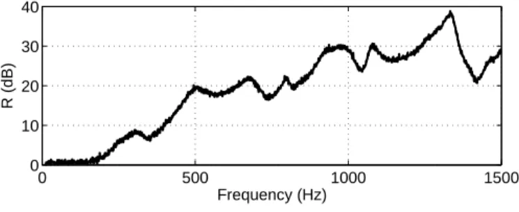
illustrated by the value of the Hsindicator R as introduced in section 3.5. This
indicator R is equal to 0dB below 200Hz, which means that the n and n + 1th
eigenvalues are about the same level. It is thus hard to separate signal from noise. Above 200Hz, the ratio becomes significantly greater than 1, resulting in a better estimation. 0 500 1000 1500 0 10 20 30 40 Frequency (Hz) R (dB)
Fig. 3. Hs indicator R given by equation (23)
In the current case, an equal amount of noise is used on all outputs to simulate
measurement noise. For this reason Hs with equal scaling factors gives the
best estimate, as can be seen from Figure 2. In case different signal-to-noise ratios are present for the indicator responses Y and the output responses X, a different scaling factor for the indicator responses Y and the output responses
X, respectively, would in that situation give the best Hs estimate.
5 Experimental illustration
An experimental validation has been carried out to validate the proposed approach. The experiment took place in two rooms which are acoustically connected with each other by means of an aluminum plate with a thickness of 1mm and a dimension of 60 x 40 cm. Twenty microphones –the set of output responses– were placed on the reception room side. The plate was excited from the emission room side by means of two shakers and one loudspeaker, consti-tuting two structure borne paths and one airborne path. Two accelerometers were mounted on the plate, near shaker connection points, and one micro-phone was placed in the emission room : these three responses were chosen as indicators (the accelerometers for the two shakers and the microphone for the loudspeaker). In a first step, each source has been excited successively with white noise to measure directly transfer functions between inputs (signals sent to the shakers and loudspeaker) and responses, to build matrices H and Φ.
For each excitation configuration with only one active source, the transfer
functions have been estimated using a H1 approach, which is well suited for
transfer function measurements with a low noise on inputs. This assump-tion seems reasonable because input signals are directly measured (without acoustic or vibration transmission) and because they are white (the energy is distributed continuously on the whole frequency range). The transmissibil-ity matrix assessed with H and Φ (equation 2) is considered as the reference transmissibility matrix in the following.
In a second step, the three physical sources were driven by three uncorrelated generators simultaneously to measure the whole response cross-spectral
ma-trix Gxyxy. H1 and H2 estimators of the transmissibility matrix have been
assessed, as well ad Hs. For the latter, a scaling has to be applied because
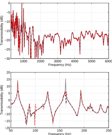
dif-ferent kinds of sensors are used (accelerometers and microphones). The scaling strategy was to normalize all measurement channel by its rms value, thus as-suming that the SNR ratio is the same on all channels. One element of the transmissibility matrix is drawn in Figure 4. All estimators fit the reference transmissibility well on the whole frequency range, even if some errors are visible in low frequency.
1000 2000 3000 4000 5000 6000 −30 −25 −20 −15 −10 −5 0 Frequency (Hz) Transmissibility (dB) 50 100 150 200 250 −20 −15 −10 −5 0 5 10 15 20 Frequency (Hz) Transmissibility (dB)
Fig. 4. #(5,2) element of the transmissibility matrix, whole (top) and low (bottom) frequency ranges. Solid gray : T based on reference measurements, H1(dotted blue),
H2 (dash-dotted black) and Hs (dashed red) estimates
drawn in Figure 5. It is clear that the estimation error is significantly lower
with the Hsestimator on the whole frequency range. In low frequency, Hsand
H2 are similar, and globally better than H1. In the high frequency range, Hs
is similar to H1, even slightly better, and both are significantly better than
H2.
It can be said globally that the Hs estimator gives better results in this
ex-periment than H1 and H2. The applied scaling strategy (normalization of the
global levels) was however very basic, and could be improved and optimized to obtain even more satisfying results.
0 1000 2000 3000 4000 5000 6000 10−3 10−2 10−1 100 Frequency (Hz) T relative error
Fig. 5. 500Hz frequency band integrated relative errors of H1 (dotted blue), H2
(dash-dotted black) and Hs (dashed red) estimates.
The relative error of Hs is drawn in Figure 6 (top) in narrow frequency bands
in the low frequency range, together with the R indicator defined in equation (23). It can be seen that the indicator is in good agreement with the estimation error : it can be said roughly that when the indicator is greater than 10dB, then the relative estimation error is below 10%. On the other hand, when the indicator drops to almost 0dB, then the relative error increases and can exceed 100%.
Conclusion
Transmissibility matrices are generally estimated using a H1 like approach.
The possibility to use H2 and Hs estimators for transmissibility matrices is
presented. The Hs approach is particularly interesting for the estimation of
transmissibility matrices, because the inputs and outputs of a transmissibil-ity system are both responses, the SNR (Signal to Noise Ratio) has thus no
reason to be higher on input or output responses. The Hs estimate of the
transmissibility matrix is based on the eigenvalue decomposition of the global cross spectral matrix of input and output responses. After a rigorous
50 100 150 200 250 10−2 10−1 100 Relative error (E s ) 50 100 150 200 250 0 10 20 30 R (dB) Frequency (Hz)
Fig. 6. Relative errors of Hs[T ] (top) and corresponding SNR indicator (bottom) in
the low frequency range.
to H1 and H2, depending on the scaling ratios. It is worth nothing that the
estimator H2 only exists if the number of output dofs m is equal or larger
than the number of indicator dofs n. Both a numerical simulation and a phys-ical experiment have been conducted to validate the proposed transmissibility estimates. In the numerical simulation a simply supported rectangular plate was considered. In the experiment a plate was excited by means of two shakers and one loudspeaker, constituting two structure borne paths and one airborne path. Both accelerometers and microphones were used, which required some
scaling of the data in order to optimize the Hs estimate. For both the
nu-merical simulation and the physical experiment it was found that Hs behaves
globally better than H1 and H2. In addition, an indicator for the validity of
Hs is introduced, which checks that there is a clear separation between the n
largest eigenvalues (representing the signal), and the m remaining eigenvalues (representing noise). By approximation, and at least for numerical and experi-mental illustrations presented in this work , it can be said that for values of the indicator larger than 10dB, the relative error in the transmissibility estimate is below 10%.
Appendix A : simulation of cross-spectral matrices of uncorrelated finite gaussian signals estimated by the periodogram method
The aim of this appendix is to explain how cross spectral matrices are ran-domly generated for measurement simulations. Studied signals are considered to be Gaussian :
x[n] =N (0 ; x) ,
where x stands for the rms value of the signal. The discrete Fourier Transform of x is given by Xk= 1 N N −1 X n=0 x[n]e−j2πkn/N
with the following expected value and variance
E(Xk) = 0 V(Xk) = x2/N
with E(Xk) = 0 and V(Xk) = x2/N . Xk follows a complex gaussian law for
k 6= {0, N/2}, the real and imaginary parts following real centered gaussian
laws of variance x2
/2N . For k ={0, N/2} , Xk follows a real centered gaussian
law of variance x2
/N , but this case will not be treated here for the sake of
brevity. The double sided instantaneous autospectrum for k 6= {0, N/2} is
equal to Sxxi k = 2|Xk| 2 = 2R (Xk) 2 + 2I (Xk) 2 = x 2 Nχ 2 2
with the following expected value and variance
E(Sxxi k) = 2x2 N V(S i xxk) = 4x4 N2
The expected value and variance of the double sided instantaneous cross
spec-trum Si
xyk = 2XkY
∗
k of two independent signals x and y are
E(Sxyi k) = 0 V(S i xyk) = 4x2 y2 N2
When applying the averaged periodogram method, auto and cross spectra are averaged over a number M of time windows :
Sxxk =h|Xk|
2
iM Sxyk =hXkYkiM
Assuming that M is sufficiently high to apply the central limit theorem, then averaged auto and cross spectra are following gaussian distributions :
Sxxk =N Ã 2x2 N ; 2x2 N√M ! Sxyk =N Ã 0 ; 2x y N√M ! , k ∈]0, N/2[
It is finally possible to simulate whole cross spectral matrices of uncorrelated signals using a gaussian random generator, from signals rms values, fixing values for N (number of samples of a time window) and M (number of time windows).
References
[1] S. Chesn´e, A. Deraemaeker, and A. Preumont. On the transmissibility functions and their use for damage localization. In International Workshop on Structural
Health Monitoring (IWSHM 09), Stanford, CA, USA, 2009.
[2] C. Devriendt and P. Guillaume. The use of transmissibility measurements in output-only modal analysis. Mechanical Systems and Signal Processing, 21(7):2689 – 2696, 2007.
[3] C. Devriendt, G. De Sitter, and P. Guillaume. An operational modal analysis approach based on parametrically identified multivariable transmissibilities.
Mechanical Systems and Signal Processing, 24(5):1250 – 1259, 2010. Special
Issue: Operational Modal Analysis.
[4] P. Gajdatsy, K. Janssens, Wim Desmet, and H. Van der Auweraer. Application of the transmissibility concept in transfer path analysis. Mechanical Systems
and Signal Processing, 24(7):1963 – 1976, 2010. Special Issue: ISMA 2010.
[5] N. B. Roozen, Q. Leclere, and C. Sandier. Operational transfer path analysis applied to a small gearbox test set-up. In proceedings of Acoustics 2012, Nantes, France, 2012.
[6] A.M.R. Ribeiro, J.M.M. Silva, and N.M.M. Maia. On the generalisation of the transmissibility concept. Mechanical Systems and Signal Processing, 14(1):29 – 35, 2000.
[7] J.S. Bendat and A.G. Piersol. Engineering applications of correlation and spectral analysis. Wiley-Interscience, New York, 1980.
[8] A.L. Wicks and H. Vold. The hs frequency response function estimator. In
Proc. 4th Int. Modal Analysis Conf., Los Angeles, CA, USA, 1986.
[9] P.R. White and W.B. Collis. Analysis of the tls frequency response function estimator. In Proceedings of the Ninth IEEE workshop on Statistical Signal
Processing, Portland OR, USA, 1998.
[10] M.H. Tan and J.K. Hammond. A non-parametric approach for linear system identification using principal component analysis. Mechanical Systems and
Signal Processing, 21(4):1576 – 1600, 2007.
[11] S.M. Price and R.J. Bernhard. Virtual coherence : A digital signal processing technique for incoherent source identification. In Proceedings of IMAC 4, Schenectady, NY, USA, 1986.
[12] Q. Leclere, C. Pezerat, B. Laulagnet, and L. Polac. Different least squares approaches to identify dynamic forces acting on an engine cylinder block. Acta
Acustica, 90:285–292, 2004.
[13] Q. Leclere, C. Pezerat, B. Laulagnet, and L. Polac. Indirect measurement of main bearing loads in an operating diesel engine. Journal of Sound and


![Fig. 6. Relative errors of H s [T ] (top) and corresponding SNR indicator (bottom) in the low frequency range.](https://thumb-eu.123doks.com/thumbv2/123doknet/14367617.503845/15.892.225.619.125.423/fig-relative-errors-corresponding-snr-indicator-frequency-range.webp)
