Collision-Free Hashing from Lattice Problems

Collision-Free Hashing from Lattice Problems

The MIT Faculty has made this article openly available.

Please share

how this access benefits you. Your story matters.

Citation

Goldreich, Oded, et al. “Collision-Free Hashing from Lattice

Problems.” Studies in Complexity and Cryptography. Miscellanea

on the Interplay between Randomness and Computation, edited by

Oded Goldreich, vol. 6650, Springer Berlin Heidelberg, 2011, pp. 30–

39.

As Published

http://dx.doi.org/10.1007/978-3-642-22670-0_5

Publisher

Springer Nature

Version

Author's final manuscript

Citable link

https://hdl.handle.net/1721.1/121244

Terms of Use

Creative Commons Attribution-Noncommercial-Share Alike

Oded Goldreich, Shafi Goldwasser, and Shai Halevi

Abstract. In 1995, Ajtai described a construction of one-way functions whose security is equivalent to the difficulty of some well known approxi-mation problems in lattices. We show that essentially the same construc-tion can also be used to obtain collision-free hashing. This paper contains a self-contained proof sketch of Ajtai’s result.

Keywords: Integer Lattices, One-EWay Functions, Worst-Case to Average-Case Reductions, Collision-Resistent Hashing.

An early version of this work appeared as TR96-042 of ECCC. The current revision is intentionally minimal.

1

Introduction

In 1995, Ajtai described a problem that is hard on the average if some well-known lattice problems are hard to approximate in the worst case, and demonstrated how this problem can be used to construct one-way functions [1]. We show that Ajtai’s method can also be used to construct families of collision-free hash functions. Furthermore, a slight modification of this construction yields families of functions which are both universal and collision-free.

1.1 The Construction

The construction is very simple. For security parameter n, we pick a random n×m matrix M with entries from Zq, where m and q are chosen so that n log q <

m < _2nq4 and q = O(n

c_{) for some constant c > 0 (e.g., m = n}2_{, q = n}7_).

See Section 3 for a discussion of the choice of parameters. The hash function hM : {0, 1}m→ Znq is then defined, for s = s1s2· · · sm∈ {0, 1}m, as

hM(s) = M s mod q =

X

i

siMimod q, (1)

where Mi is the ith column of M .

Notice that hM’s input is m-bit long, whereas its output is n log q bits long.

Since we chose the parameters such that m > n log q, there are collisions in hM.

As we will argue below, however, it is infeasible to find any of these collisions unless some well known lattice problems have good approximation in the worst case. It follows that, although it is easy to find solutions for the equations M s ≡ 0 (mod q), it seems hard to find binary solutions (i.e., a vector s ∈ {0, 1}m_{in the}

Remark. Using our notation, the candidate one-way function introduced by Ajtai is f (M, s)def= (M, hM(s)). We note that this function is regular (cf., [3]); that

is, the number of preimage of any image is about the same. (Furthermore, for most M ’s the number of pre-images under hM of almost all images is about the

same.) To the best of our knowledge, it is easier (and more efficient) to construct a pseudo-random generator based on a regular one-way function than based on an arbitrary one-way function (cf., [3] and [4]).

1.2 A Modification

A family of hash functions is called universal if a function uniformly selected in the family maps every two images uniformly on its range in a pairwise indepedent manner [2]. To obtain a family of functions that is both universal and collision-free, we slightly modify the foregoing construction. First we set q to be a prime of the desired size. Then, in addition to picking a random matrix M ∈ Zn×m

q ,

we also pick a random vector r ∈ Zn

q. The function hM,r: {0, 1}m→ Znq is then

defined, for s = s1· · · sm∈ {0, 1}m, as

hM(s) = M s + r mod q = r +

X

i

siMimod q. (2)

The modified construction resembles the standard construction of universal hash functions [2], with calculations done over Zq instead of over Z2.

2

Formal Setting

In this section we give a brief description of some well known lattice problems, outline Ajtai’s reduction, and our version of it.

2.1 Lattices

Definition 1: Given a set of n linearly independent vectors in Rn_{, denoted}

V = hv1, · · · , vni, we define the lattice spanned by V as the set of all possible

linear combinations of thevi’s with integral coefficients; that is,

L(V )def= ( X i aivi : ai∈ Z for all i ) . (3) We callV the basis of the lattice L(V ). We say that a set of vectors, L ⊂ Rn_{, is}

a lattice if there is a basisV such that L = L(V ).

It is convenient to view a lattice L in Rn_{as a “tiling” of the space R}n_{using small}

parallelepipeds, with the lattice points being the vertices of these parallelepipeds. The parallelepipeds themselves are spanned by some basis of L. We call the parallelepiped that are spanned by the “shortest basis of L” (the one whose vectors have the shortest Euclidean norm) the basic cells of the lattice L. See Figure 1 for an illustration of these terms in a simple lattice in R2_.

R2

A lattice in

Tiling using the "basic-cells" Tiling using some other basis Fig. 1.Tiling of a simple lattice in R2 _{with two different bases}

Computational problems regarding lattices. Finding “short vectors” (i.e., vectors with small Euclidean norm) in lattices is considered a hard problem. There are no known efficient algorithms to find, given an arbitrary basis of a lattice, either the shortest non-zero vector in the lattice, or another basis for the same lattice whose longest vector is as short as possible. No efficient algorithms are known for approximation versions of these problems as well. The approximation versions being considered here are the following:

(W1) Given an arbitrary basis B of a lattice L in Rn_{, approximate (up to a}

polynomial factor in n) the length of the shortest vector in L.

(W2) Given an arbitrary basis B of a lattice L in Rn_{, find another basis of L}

whose length is at most polynomially (in n) larger than that of the smallest basis of L (where the length of a basis is the length of its longest vector). We choose ‘W’ for the foregoing notation to indicate that we will be interested in the worst-case complexity of these problems. The best known algorithms for these problems are the L3 _{algorithm and Schnorr algorithm. The L}3 _algorithm,

due to Lenstra, Lenstra and Lov´asz [5] approximates these problems to within a ratio of 2n/2 _{in the worst case, and Schnorr’s algorithm [6] improves this}

to (1 + ε)n _{for any fixed ε > 0. Another problem, which can be shown to be}

equivalent to the above approximation problems (cf. [1]), is the following: (W3) Given an arbitrary basis B of a lattice L, find a set of n linearly

than the length of the smallest set of n linearly independent lattice vectors. (Again, the length of a set of vectors is the length of its longest vector.) A few remarks about (W3) are in order:

1. Note that not every linearly independent set of n lattice points is a basis for that lattice. For example, if V = {v1, v2} span some lattice in R2, then the

set {2v1, v2} is a linearly independent set of 2 vectors that does not span

L(V ), since we cannot represent v1 as an integral linear combination of 2v1

and v2.

2. In the sequel we reduce the security of our construction to the difficulty of solving Problem (W3). It will be convenient to use the following notation: For a given polynomial Q(·), denote by (W3)Qthe problem of approximating

the smallest independent set in an n-dimensional lattice up to a factor of Q(n).

2.2 Ajtai’s Reduction

In his paper Ajtai described the following problem:

Problem (A1): For parameters n, m, q ∈ N such that n log q < m ≤ _2nq4 and

q = O(nc_{), for some constant c > 0.}

Input: A matrix M ∈ Zn×m q .

Output: A vector x ∈ Zm

q \ {0m} such that M x ≡ 0 (mod q) and kxk < n

(where kxk denotes the Euclidean norm of x).

Here, we used ‘A’ (in the notation) to indicate that we will be interested in the average-case complexity of this problem. Ajtai proved the following theorem, reducing the worst-case complexity of (W3) to the average-case complexity of (A1).

Ajtai’s Theorem [1]: Suppose that it is possible to solve a uniformly se-lected instance of Problem (A1) in expected T (n, m, q)-time, where the expec-tation is taken over the choice of the instance as well as the coin-tosses of the solving algorithm. Then, it is possible to solve Problem (W3) in expected poly(|I|) · T (n, poly(n), poly(n)) time on every n-dimensional instance I, where the expectation is taken over the coin-tosses of the solving algorithm.

Remark. Ajtai [1] has noted that the theorem remain valid also when Prob-lem (A1) is relaxed so that the desired output is allowed to have Euclidean norm of up to poly(n) (i.e., one requires kxk ≤ poly(n) rather than kxk < n). 2.3 Our Version

We observe that one can use essentially the same proof to show that the following problem is also hard on the average.

Problem (A2): For parameters n, m, q ∈ N as in (A1). Input: A matrix M ∈ Zn×m

q .

Output: A vector x ∈ {−1, 0, 1}m_{\ {0}m_{} such that M x ≡ 0 (mod q).}

Theorem 1: Suppose that it is possible to solve a uniformly selected instance of Problem(A2) in expected T (n, m, q)-time, where the expectation is taken over the choice of the instance as well as the coin-tosses of the solving algorithm. Then, it is possible to solve Problem(W3) in expected poly(|I|) · T (n, poly(n), poly(n)) timeon every n-dimensional instance I, where the expectation is taken over the coin-tosses of the solving algorithm.

Proof: By the foregoing Remark, Ajtai’s Theorem holds also when modify-ing Problem (A1) such that the output is (only) required to have Euclidean norm of up to m. Once so modified, Problem (A1) becomes more relaxed than Problem (A2) and so the current theorem follows.

For the sake of self-containment we sketch the main ideas of the proof of Ajtai’s Theorem (equivalently, of Theorem 1) in Section 4. The reader is referred to [1] for further details.

3

Constructing Collision-Free Hash Functions

The security of our proposed collision-free hash functions follows directly from Theorem 1. Below, we spell out the argument and discuss the parameters. 3.1 The functions and their security

Recall our construction of a family of collision-free hash functions: Picking a hash-function

To pick a hash-function with security-parameters n, m, q (where n log q < m ≤_2nq4 and q = O(n

c_{)), we pick a random matrix M ∈ Z}n×m q .

Evaluating the hash function Given a matrix M ∈ Zn×m

q and a string s ∈ {0, 1}m, compute

hM(s) = M s mod q =

X

i

siMimod q.

The collision-free property is easy to establish assuming that Problem (A2) is hard on the average. That is:

Theorem 2: Suppose that given a uniformly chosen matrix, M ∈ Zn×m q , it

is possible to find in (expected) T (n, m, q)-time two vectors x 6= y ∈ {0, 1}m

such thatM x ≡ M y (mod q). Then, it is possible to solve a uniformly selected instance of Problem (A2) in (expected) T (n, m, q)-time.

Proof: If we can find two binary strings s1 6= s2∈ {0, 1}msuch that M s1≡

M s2 (mod q), then we have M (s1− s2) ≡ 0 (mod q). Since s1, s2∈ {0, 1}m,

we have x def= (s1− s2) ∈ {−1, 0, 1}m, which constitutes a solution to

3.2 The Parameters

The proof of Theorem 1 imposes restrictions on the relationship between the parameters n, m and q. First of all, we should think of n as the security parameter of the system, since we derive the difficulty of solving Problem (A2) by assuming the difficulty of approximating some problems over n-dimensional lattices.

The condition m > n log q is necessary for two reasons. The first is simply because we want the output of the hash function to be shorter than its input. The second is that when m < n log q, a random instance of problem (A2) typically does not have a solution at all, and the reduction procedure in the proof of Theorem 1 falls apart.

The conditions q = O(nc_{) and m < q/2n}4 _{also come from the proof of}

Theorem 1. Their implications for the security of the system are as follows: – The larger q is, the stronger the assumption that needs to be made

regard-ing the complexity of problem (W3). Namely, the security proof shows that (A2) with parameters n, m, q is hard to solve on the average, if the prob-lem (W3)(qn6₎ is hard in the worst case, where (W3)_(qn6₎ is the problem of

approximating the shortest independent set of a lattice up to a factor of qn6_.

Thus, for example, if we worry (for a given n) that an approximation ratio of n15 _{is feasible, then we better choose q < n}9_{. Also, since we know that}

approximation within exponential factor is possible, we must always choose q to be sub-exponential in n.

– By the above, the ratio Rdef= q/n_m4 must be strictly bigger than 1 (above, for simplicy, we stated R > 2). The larger R is, the better the reduction becomes: In the reduction from (W3) to (A2) we need to solve several random (A2) problems to obtain a solution to one (W3) problem. The number of instances of (A2) problem which need to be solved depends on R. Specifically, this number behaves roughly like n2_{/ log R. This means that when q/n}4 _{= 2m}

we need to solve about n2_{instances of (A2) per any instance of (W3), which}

yields a ratio of O(n2_{) between the time it takes to break the hashing scheme}

and the time it takes to solve a worst-case (W3) problem. On the other hand, when R approaches 1 the number of iterations (in the reduction) grows rapidly (and tends to infinity).

Notice also that the inequalities n log q < m < _nq4 implies a lower bound on q,

namely _{log q}q > n5_{, which means that q = Ω(n}5_{log n).}

4

Self-contained Sketch of the Proof of Theorem 1

At the heart of the proof is the following procedure for solving (W3): It takes as inputs a basis B = hb1, · · · , bni for a lattice and a set of n linearly independent

lattice vectors V = hv1, · · · , vni, with |v1| ≤ |v2| ≤ · · · ≤ |vn|. The procedure

produces another lattice vector w, such that |w| ≤ |vn|/2 and w is linearly

independent of v1, · · · , vn−1. We can then replace the vector vn with w and

this procedure, we denote by S the length of the vector vn (which is the longest

vector in V ).

In the sequel we describe this procedure and show that as long as S is more than nc _{times the size of the basic lattice-cell (for some constant c > 0), the}

procedure succeeds with high probability. Therefore we can repeat the process until the procedure fails, and then conclude that (with high probability) the length of the longest vector in V is not more that nc _{times the size of the basic}

lattice-cell. For the rest of this section we will assume that S is larger than nc

times the size of the basic lattice-cell.

The procedure consists of five steps: We first construct an “almost cubic” parallelepiped of lattice vectors, which we call a pseudo-cube. Next, we divide this pseudo-cube into qn_{small parallelepipeds (not necessarily of lattice vectors),}

which we call sub-pseudo-cubes. We then pick some random lattice points in the pseudo-cube (see Step 3) and consider the location of each point with respect to the partition of the pseudo-cube into sub-pseudo-cubes (see Step 4). Each such location is represented as a vector in Znq and the collection of these vectors

forms an instance of Problem (A2). A solution to this instance yields a lattice point that is pretty close to a “corner” of the pseudo-cube. Thus, our final step consists of using the solution to this (A2) instance to compute the “short vector” w. Below we describe each of these steps in more details.

1. Constructing a “pseudo-cube”. The procedure first constructs a paral-lelepiped of lattice vectors that is “almost a cube”. This can be done by taking a sufficiently large cube (say, a cube with side length of n3_{S), expressing each of}

the cubes’ basis vectors as a linear combination of the vi’s, and then rounding

the coefficients in this combination to the nearest integers. Denote the vectors thus obtained by f1, · · · , fn and the parallelepiped that is spanned by them by

C. The fi’s are all lattice vectors, and their distance from the basis vectors of

the “real cube” is very small compared to the size of the cube. 1 _{Hence the}

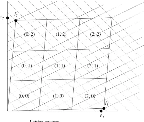
parallelepiped C is very “cube-like”. We call this parallelepiped a pseudo-cube. 2. Dividing the pseudo-cube into “sub-pseudo-cubes”. We then divide C into qn _{equal sub-pseudo-cubes, each of which can be represented by a vector}

in Zn q as follows: for every T =    t1 .. . tn   ∈ Z n q, define CT def= ( X i αifi : ti q ≤ αi< ti+ 1 q ) .

For each sub-pseudo-cube CT, we call the vector oT =

P

it

i

qfi the origin of CT

(i.e., oT is the vector in CT that is closest to the origin). We note that any vector

in v ∈ CT can be written as v = oT + δ where δ is the location of v inside the

1 _{The f}

i’s can be as far as Sn/2 away from the basis vectors of the real cube, but this

e

Lattice vectors

e

f , f

e

, e

f

f

The "real cube"

(0, 0)

(0, 1)

(1, 1)

(2, 1)

(1, 2)

(2, 2)

(0, 2)

(1, 0)

(2, 0)

The pseudo-cube

Fig. 2.The basic construction in the proof of Theorem 1 (for q = 3)

sub-pseudo-cube CT. See Figure 2 for an illustration of that construction (with

n = 2, q = 3).

The parameter q was chosen such that each CT is “much smaller” than S.

That is, the side-length of each sub-pseudo-cube CT is Sn3/q ≤ S/2nm. On the

other hand, with this choice, each CT is still much larger than the basic lattice

cell (since S is much bigger than the size of the basic cell). This, together with the fact that the CT’s are close to being cubes, implies that each CT contains

approximately the same number of lattice points.

3. Choosing random lattice points in C. We then choose m random lattice points u1, · · · um ∈ C. To do that, we use the basis B = {b1, · · · , bn} of the

lattice. To choose each point, we take a linear combination of the basis vectors bi with large enough integer coefficients (say, in the range [0, 2n

c

· max(S, |B|)] for some constant c). This gives us some lattice point p.

We then “reduce p mod C”. By this we mean that we look at a tiling of the space Rn _{with the pseudo-cube C, and we compute the location vector of}

p in its surrounding pseudo-cube. Formally, this is done by representing p as a linear combination of the fi’s, and taking the fractional part of the coefficients

in this combination. The resulting vector is a lattice point, since it is obtained by subtracting integer combination of the fi’s from p, whereas the fi’s are lattice

vectors. Also, this vector must lie inside C, since it is a linear combination of the fi’s with coefficients in [0, 1). It can be shown that if we choose the coefficients

from a large enough range, then the distribution induced over the lattice points in C is statistically close to the uniform distribution.

4. Constructing an instance of Problem (A2). After we have chosen m lat-tice points u1, · · · , um, we compute for each ui the vector Ti∈ Znq that represent

the sub-pseudo-cube in which ui falls. That is, for each i we have ui∈ CTi.

Since, as we said above, each sub-pseudo-cube contains approximately the same number of points, and since the ui’s are distributed almost uniformly in C,

then the distribution induced on the CTi’s is close to the uniform distribution,

and so the distribution over the Ti’s is close to the uniform distribution over Znq.

We now consider the matrix whose columns are the vectors Ti, that is,

M = (T1|T2| · · · |Tm). By the foregoing argument, it is an “almost uniform”

random matrix in Zn×m

q , and so, it is an “almost uniform” random instance of

Problem (A2).

5. Computing a “short lattice vector”. We now have a random instance M of Problem (A2), and so we can use the algorithm whose existence we assume in Theorem 1 to solve this instance in expected T (n, m, q) time. The solution is a vector x = {x1, · · · , xm} ∈ {−1, 0, 1}msuch that M x =PixiTi is congruent

to 0 mod q.

Once we found x, we compute the lattice vector w′

= Pm

i=1xiui. Let us

examine the vector w′

: Recall that we can represent each ui as the sum of

oi def= oTi (the origin vector of CTi) and δi (the location of ui inside CTi). Thus,

w′ = m X i=1 xiui= m X i=1 xioi+ m X i=1 xiδi.

A key observation is that since P

ixiTi ≡ ¯0 (mod q), “reducing the vector

(P

ixioi) mod C” yields the all-zeros vector; that is, (Pixioi) mod C = ¯0. To

see why this is the case, recall that each oi = oTi has the form

P

j ti(j)

q fj,

where ti(j) ∈ {0, ..., q − 1} is the jth component of Ti. Now, the hypothesis

P

ixiti(j) ≡ 0 (mod q) for j = 1, .., n, yields that

X i xioTi = X i xi X j ti(j) q fj = X j P ixiti(j) q fj = X j cjfj

where all cj’s are integers. Since “reducing the vectorPixioTi mod C” means

subtracting from it an integer linear combination of fj’s, the resulting vector is

¯0. Thus, “reducing w′

mod C” we getPm

i=1xiδi; that is,

w′ mod C = m X i=1 xiδi.

Since each δi is just the location of some point inside the sub-pseudo-cube CTi,

the size of each δi is at most n · S/2mn = S/2m. Moreover as xi∈ {−1, 0, 1} for

all i we get X i xiδi ≤X i |xi| · kδik ≤ m · S 2m= S 2.

This means that the lattice vector w′

mod C is close up to S

2 to one of the

“corners” of C. Thus, all we need to do is to find the difference vector between the lattice vector w′

mod C and that corner (which is also a lattice vector). Doing that is very similar to reducing w′

mod C: We express w′

as a linear combination of the fi’s, but instead of taking the fractional part of the coefficients, we take

the difference between these coefficients and the closest integers. This gives us the “promised vector” w, a lattice vector whose length is at most S/2.

The only thing left to verify is that with high probability, w can replace the largest vector in V (i.e., it is linearly independent of the other vectors in V ). To see that, notice that the vector x does not depend on the exact choice of the ui’s, but only on the choice of their sub-pseudo-cubes CTi’s. Thus, we can think

of the process of choosing the ui’s as first choosing the CTi’s, next computing

the xi’s and only then choosing the δi’s.

Assume (w.l.o.g.) that we have x16= 0. Let us now fix all the δi’s except δ1

and then pick δ1so as to get a random lattice point in CT1. Thus, the probability

that w falls in some fixed subspace of Rn _{(such as the one spanned by the n − 1}

smallest vectors in V ), equals the probability that a random point in CT1 falls

in such subspace. Since CT1 is a pseudo-cube that is much larger than the basic

cell of L, this probability is very small.

Acknowledgments

We thank Dan Boneh and Jin Yi Cai for drawing our attention to an error in a previous version of this note.

References

1. M. Ajtai. Generating Hard Instances of Lattice Problems. In 28th ACM Symposium on Theory of Computing, pages 99–108, Philadelphia, 1996.

2. L. Carter and M. Wegman. Universal Classes of Hash Functions. J. Computer and System Sciences, Vol. 18, pages 143–154, 1979.

3. O. Goldreich, H. Krawczyk and M. Luby. On the existence of pseudorandom generators. SIAM J. on Computing, Vol. 22-6, pages 1163–1175, 1993.

4. J. H˚astad, R. Impagliazzo, L.A. Levin and M. Luby. A Pseudorandom Generator from any One-way Function. SIAM J. on Computing, Vol. 28 (4), pages 1364–1396, 1999. Combines papers of Impagliazzo et al. (21st STOC, 1989) and H˚astad (22nd STOC, 1990).

5. A.K. Lenstra, H.W. Lenstra, L. Lov´asz. Factoring Polynomials with Rational Coefficients. Mathematische Annalen 261, pages 515–534, 1982.

6. C.P. Schnorr. A more efficient algorithm for a lattice basis reduction. Journal of Algorithms, Vol. 9, pages 47–62, 1988.