PSFC/JA-03-14
Coherent Acceleration of Magnetized Ions
by Electrostatic Waves With Arbitrary Wavenumbers
D. J. Strozzi, A. K. Ram, and A. BersJune 2003
Plasma Science and Fusion Center Massachusetts Institute of Technology
Cambridge, MA 02139 U.S.A.
This work was supported by the U.S. Department of Energy, Grant No. DE-FG02-91ER-54109, by the U.S. Department of Energy jointly with the National Science Foundation, Grant No. DE-FG02-99ER-54555, by the National Science Foundation, Grant No. ATM-0114462, and by Princeton University, Subcontract 150-6804-1. Reproduction, translation, publication, use and disposal, in whole or in part, by or for the United States government is permitted.
Coherent acceleration of magnetized ions by electrostatic waves
with arbitrary wavenumbers
D. J. Strozzi,∗ A. K. Ram, and A. Bers
Plasma Science and Fusion Center,
Massachusetts Institute of Technology, Cambridge, Massachusetts 02139
(Dated: July 3, 2003)
Abstract
This paper studies the coherent acceleration of ions interacting with two electrostatic waves in a uniform magnetic field ~B0. It generalizes an earlier analysis of waves propagating perpendicularly
to ~B0 to include the effect of wavenumbers along ~B0. The Lie transformation technique is used to develop a perturbation theory describing the ion motion, and results are compared with numerical solutions of the complete equations of motion. Coherent energization occurs when the Doppler-shifted wave frequencies differ by nearly an integer multiple of the ion cyclotron frequency. When the difference in the parallel wavenumbers of the two waves is increased the coherent energization of ions is limited to a small part of the phase space. The energization of ions and its dependence on wave parameters is discussed.
PACS numbers: 05.45.-a, 45.50-j, 52.20.Dq, 52.50.Sw
Keywords: wave-particle interactions, coherent ion energization, Lie-transform method
I. INTRODUCTION
The motion of charged particles in the presence of electromagnetic waves is a rich dynam-ical system that has been studied for a variety of cases. Important physdynam-ical applications of this problem occur in laboratory and space plasmas, such as for high-temperature (collision-less) plasma heating and current drive and the transverse energization of ions for times short compared to collisional times. A particular area of interest is the nonlinear heating of ions (as opposed to linear mechanisms such as Landau and cyclotron damping) by electrostatic waves propagating through a plasma in a uniform magnetic field ~B0.
For a single electrostatic wave propagating across ~B0, the stochastic heating of ions by
waves with frequency ω À ωcibut ω 6= Nωci (where N is an integer and ωci≡ qB0/M is the
ion cyclotron frequency) was studied by Karney and Bers [1, 2]. It was found that ions with speeds across ~B0 less than the phase velocity of the wave ω/k⊥(that is, k⊥ρi & ω/ωci) exhibit
regular motion and do not gain energy. However, for wave amplitudes above a threshold amplitude, the ions are stochastically heated if their speeds are inside a region with a lower bound near ω/k⊥. The stochastic “webs” generated by a single perpendicularly propagating
wave with frequency ω = Nωci also lead to stochastic ion heating [3–5].
For a single wave propagating obliquely to ~B0 it was found that ions could also be
stochastically heated [6, 7]. It has recently been shown that single and multiple drift-Alfv´en waves with ω < ωci can induce stochastic ion heating [8], which may account for certain
experimental observations [9]. For two waves propagating obliquely to ~B0, the threshold
wave amplitudes needed for stochastic motion can be significantly lowered [10]. There is still a lower bound for the stochastic region of phase space.
For two perpendicular waves that satisfy the resonance condition ω1 − ω2 = Nωci Ram
et al. discovered numerically [11] that coherent (as opposed to chaotic) energization can bring ions from low energies into the stochastic domain. B´enisti et al. [12] then showed that this coherent energization was described by perturbation analysis using Lie transformation methods. The coherent energization was also shown by Ram et al. [13] to be described by a multiple time scale analysis, and invoked to explain the energization of hydrogen and oxygen ions from Earth’s upper auroral ionosphere into the magnetosphere. For two non-collinear, perpendicularly propagating waves, the coherent energization was found to persist as long as the angle between them was less than 30◦ [14].
Coherent acceleration by electrostatic waves with ω1 − ω2 = Nωci can only occur when
both wave frequencies are larger than ωci. This process is most interesting for cases where
ions with energy well below the stochastic region (k⊥ρi ¿ ω/ωci) are accelerated into it.
Most of the work on coherent acceleration has focused on waves with frequencies much higher than ωci. In magnetic fusion experiments and in the Earth’s ionosphere, lower-hybrid
waves fit this description (ωlh ∼ ωpi À ωci, ωlh = lower-hybrid frequency, ωpi = ion plasma
frequency).
In this paper we study the interaction of ions with electrostatic waves ranging in fre-quency from lower-hybrid frequencies down to a few multiples of ωci. The analysis of B´enisti
et al. [12] is generalized to include nonzero wavenumbers along ~B0. We develop a
pertur-bation theory using the Lie transformation method and find conditions for which coherent acceleration persists. We also discuss the dependence of the range of energization and period of coherent oscillations on wave parameters.
The Hamiltonian formulation of the problem is given in Section II. An analytic perturba-tion theory for the coherent moperturba-tion based on the Lie transformaperturba-tion technique is described
in Section III. Section IV compares the results for the perturbation theory with numerical results obtained from the complete dynamical equations. The scalings of coherent ener-gization and the period of oscillation, for perpendicularly propagating waves, are obtained. Section V discusses the case of obliquely propagating waves and compares the results with those for two perpendicularly propagating waves.
II. EQUATIONS OF MOTION
The nonrelativistic equation of motion of an ion in the presence of a uniform magnetic field ~B0 = B0z in a plasma and interacting with two electrostatic waves isˆ
Md 2~x dt2 = q 2 X i=1 Φi~kisin(~ki· ~x − ωit + αi) + q~v × ~B0 (1)
where Φi is the electrostatic potential amplitude, ~ki is the wavevector, ωi is the wave
fre-quency, and αi is the phase of the ith wave. We normalize times to the inverse of the ion
cyclotron frequency ωci, distances to the inverse of k1x, and masses to the ion mass M. We
restrict our attention to the case where both ~ki’s lie in the x − z plane. Let νi ≡ ωi/ωci and
²i ≡ (ωBi/ωci)2, where ωBi ≡ (qk21xΦi/M)1/2 is the bounce frequency in the ith wave. The
Hamiltonian for this system is h(~x, ~p, t) = 1
2(~p − ~A)
2+X
i
²icos(~ki· ~x − νit + αi) (2)
where ~A = B0xˆy is the vector potential, and ~p = m~v + q ~A → ~v + xˆy is the (nondimensional)
canonical momentum.
Since h is independent of y, we can eliminate the y degree of freedom by making a Galilean transformation to a frame moving in the ˆy direction with speed py0 = vy0+ x0 (the
subscript 0 refers to a quantity’s initial value). Following Ref. [15], the generating function for the canonical transformation from (y, py) to (y0, p0y) is F2 = (y − py0t)(p0y + py0). Then
y0 = y − p
y0t and p0y = py− py0, so that p0y0= 0. The transformed Hamiltonian (to within a
constant) is h(x, z, px, p0y, pz, t) = 12 £ p2 x+ p02y + (x − py0)2+ p2z ¤ +X i ²icos(~ki· ~x − νit + αi) (3) Since ∂h0/∂y0 = 0, p0
y is independent of time so that p0y = 0. This eliminates the y0 degree
of freedom from the dynamics. Replacing x by x0 = x − p
y0 and pz by vz gives h0(x0, z, px, vz, t) = 21(p2x+ x02+ vz2) + X i ²icos(kixx0+ kizz − νit + αi) (4) where αi+ kixpy0 is replaced by αi.
In a frame moving with velocity uˆz the Hamiltonian remains unchanged except that the wave frequencies are Doppler shifted: νi → νi− kizu. Without loss of generality we assume
We transform (x0, p
x) to action-angle coordinates (φ, I) using the generating function
F1 = 12x02cot φ. Then I = 12(vx2+ x02) = 12(vx2+ vy2) is the perpendicular kinetic energy, and
φ = arctan(x0/v
x) = arctan(−vy/vx) is the gyrophase. The transformed Hamiltonian is
H(φ, z, I, vz, t) = I + 12vz2+
X
i
²icos(kixρ sin φ + kizz − νit + αi) (5)
where ρ =√2I is the ion gyroradius.
III. PERTURBATION ANALYSIS OF COHERENT MOTION
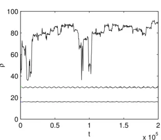
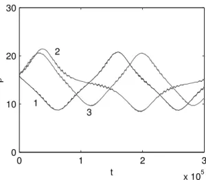
In general, the equations of motion obtained from (5) cannot be solved analytically. Consequently, we resort to numerical solutions to provide an insight into the dynamics of ions in two electrostatic waves. Figure 1 shows the time evolution of ρ for three ions having the same initial ρ0, but different φ0, interacting with two waves of frequencies ν1 = 40.37 and
ν2 = 39.37, and amplitudes ²1 = ²2 = 4. (All the numerical solutions of ordinary differential
equations have been carried out using the Bulirsch-Stoer algorithm described in Ref. [16].) There are two distinct kinds of motion: the slow, smooth, “coherent” oscillations at lower ρ, and the irregular, “stochastic” motion at higher ρ. Superimposed on the coherent motion are small-amplitude, high-frequency fluctuations. Figure 2 shows the orbits for the same parameters as Fig. 1 except that ν2 = 39.369 and the initial conditions are different. This
demonstrates that the coherent acceleration from low to high energies occurs only when ν1− ν2 is an integer.
Our interest is to provide an analytical description of the coherent dynamics without going into details of the stochastic region, other than to note its existence for ρ ≈ min(νi)
[1, 2]. We assume that the waves are perturbing the cyclotron motion of the ions and express
H = H0+ H1 (6) where H0 = I + 12vz2 and H1 = X i ²icos(kixρ sin φ + kizz − νit + αi). (7)
An approximate analytical description of the ion motion in the coherent regime is obtained by using the Lie perturbation technique [17, 18] with the ordering parameter ² (² ∼ ²1 ∼ ²2).
We assume that νi ∈ Z but (ν/ 1 − ν2) = N ∈ Z. For νi ∈ Z a web structure is formed
in phase space and has been discussed elsewhere for a single wave [4] and for two waves propagating across ~B0 [19]. For the case of a single wave the stochastic web structure also
has a lower bound [20].
From the Lie perturbation analysis (Appendix A) the Hamiltonian that describes the coherent ion motion to O(²2) is
¯
where ¯ H2 = S0( ¯I, ¯vz) + S−( ¯I, ¯vz) cos(N( ¯φ − t) + ∆kzz + α¯ 1 − α2) (9) S0 = S0x+ S0z (10) S0x = − 1 2¯ρ X i kix²2i m m − µi Jm,iJm,i0 (11) S0z = 14 X i k2 iz²2i J2 m,i (m − µi)2 (12) S− = S−x+ S−z (13) S−x = − ²1²2 4¯ρ(m − µ1) (k1x(m − N)Jm,10 Jm−N,2+ k2xmJm,1Jm−N,20 ) (14) − ²1²2 4¯ρ(m − µ2) (k1xmJm,2Jm+N,20 + k2x(m + N)Jm,20 Jm+N,1) S−z = 14k1zk2z²1²2 µ Jm,1Jm−N,2 (m − µ1)2 +Jm,2Jm+N,1 (m − µ2)2 ¶ (15) ∆kz = (k1z−k2z), µi = νi−kizv¯z, and m is summed from −∞ to +∞. Jm,i ≡ Jm(kixρ) is the¯
Bessel function of the first kind and f0(ξ) = df /dξ. The barred coordinates are related to
the original coordinates by a near-identity transformation: ( ¯φ, ¯z, ¯I, ¯vz) = (φ, z, I, vz) + O(²)
(Appendix A). For instance, the relation between I and ¯I is: I ≈ ¯I − ²i X m mJm,i m − µi cos(m ¯φ + kizz − ν¯ it + αi) (16)
The Hamiltonian ¯H is a generalization to oblique waves of the results obtained in [12] for collinear perpendicularly propagating waves. In the limit kiz → 0 the above reduces to the
description in Ref. [12]. A nonzero α1− α2 is equivalent to a shift in the initial ¯φ0 so that,
without loss of generality, we can set α1 = α2 = 0.
Our perturbation analysis assumes there are no resonances at O(²). Such resonances occur if νi is an integer, where our present analysis breaks down.
The explicit time dependence in ¯H can be eliminated by transforming from ¯φ to ¯ψ = ¯φ−t using the generating function F2 = ˜I( ¯φ − t). The transformed Hamiltonian is:
˜
H( ¯ψ, ¯z, ¯I, ¯vz) = 12v¯z2+ S0( ¯I, ¯vz) + S−( ¯I, ¯vz) cos(N ¯ψ + ∆kzz)¯ (17)
where ¯I = ˜I has replaced ˜I ( ¯I and ¯ψ are canonically conjugate). Since ˜H does not depend explicitly on time it is a constant of the motion.
Using Hamilton’s equations for ˙¯I and ˙¯vz, we find a second constant of the motion:
d dt µ ¯ vz − ∆kz N I¯ ¶ = 0 (18)
Thus, the system is integrable and the dynamics described by ˜H are not stochastic. Along an orbit, ¯vz is a function of ¯I and initial conditions only:
¯
vz = vz0+
∆kz
Therefore, S0 and S− are functions just of ¯I. Since | cos x| ≤ 1
H−≤ ˜H ≤ H+, H±( ¯I) = 12¯vz2+ S0( ¯I) ± |S−( ¯I)| (20)
For an initial condition with a given value of ˜H, ¯ρ varies between the two points where ˜H equals H+(¯ρ) or H−(¯ρ). We refer to H± as the potential barriers, since they delimit the
allowed and forbidden regions of phase space.
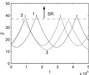
Figure 3 shows the orbits generated by the second-order Hamiltonian (17) for the same parameters as in Fig. 1. Our perturbation analysis accurately captures the coherent motion of the full system except near the stochastic region ρ ≈ min(νi) where our perturbation
theory breaks down. Below this region, ρ and ¯ρ differ by small fluctuations that are accounted for, to O(²), by the transformation (16).
IV. COHERENT MOTION FOR PERPENDICULAR WAVES
Using the Hamiltonian (17) we now analyze the ion motion for two perpendicularly prop-agating waves. Figures 1 and 3 show the complete and coherent motion, respectively, for two perpendicularly propagating waves (kiz = 0). Figure 4 displays H+ and H− from (20) for
the same parameters as in Figs. 1 and 3, and the values of ˜H for the three initial conditions. The coherent analysis correctly predicts that particle 3 in Fig. 1 will not make it into the chaotic regime because it is reflected by the bump in H−.
If we multiply ²1 and ²2 by the same factor a then ˜H in (17) is multiplied by a2 (note
that for perpendicularly propagating waves, 1
2v¯z2 is a constant and can be eliminated from
˜
H). Since a rescaling of the Hamiltonian is equivalent to a rescaling of time, rescaling both ²i’s does not affect the range of motion in ¯ρ but rescales the period by 1/a2. For ²1 ∼ ²2,
this means the period scales like 1/²2
1. This reflects the fact that the coherent motion is
second-order in the wave field amplitudes. It also shows that in certain physical situations, at sufficiently large amplitudes, the effects of collisions on the coherent energization can be made negligible.
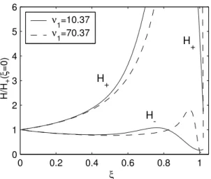
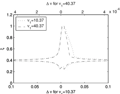
The range of coherent motion in ρ scales linearly with the wave frequencies. In Fig. 5 we plot H±/H+(ξ = 0) versus ξ ≡ ¯ρ/ν1 for two values of ν1 with N = 1. Note that the
potential barriers do not change significantly with ν1. Figure 6 shows that, as a function
of ν1, the average ξmin and ξmax have a small variation (ξmin and ξmax are the maximum
and minimum ξ attained by an ion undergoing coherent motion and occur when the ion reaches the barriers H±). The average is over ions with the same initial ξ0 = 0.4 and
different φ0 = (0, 0.05, . . . , 1)π. Waves with higher frequencies can therefore produce
co-herent energization to higher energies. Since the lower bound of the stochastic region is ρ ≈ min(νi) → ξ ≈ 1, ions with the same initial ξ0 and φ0 either will or will not reach the
stochastic region regardless of the wave frequencies. For ν1 near an integer ξmax is about
20% higher than when ν1 is near a half-integer (this is not shown explicitly in Fig. 6).
The period of oscillation in ¯I (see Fig. 3) can be estimated from the equation of motion for ˙¯I:
˙¯
I = −∂ ˜H
∂ ¯ψ = NS−sin(N ¯ψ) (21)
An orbit’s turning point typically occurs when ¯ψ = nπ/N, i.e., when it hits one of the barriers H±. Therefore, approximately, the period of oscillation τ is given by τ ≈ 2π/(Nh ˙¯ψi),
where hi denotes the average over one period. From the asymptotic forms of S0 and S− for
ν1 ∼ ν2 À 1 (Appendix B) we find that
˜
H ≈ ν−2
1 ha(ξ, ¯ψ) (22)
where ha depends on νi only through ξ. Then
˙¯ ψ = ∂ ˜H ∂ ¯I ≈ ν −2 1 ∂ha ∂ ¯I = ν −4 1 1 ξ ∂ha ∂ξ (23) Thus, τ ∼ ν4
1. Waves of lower frequency accelerate ions much more rapidly than those
with higher frequency and thus may also be made less sensitive to the effects of collisions. Figure 7 compares this scaling with the periods of two actual orbits obtained from ˜H.
V. COHERENT MOTION FOR OBLIQUE WAVES
In this section we describe the motion of ions when the waves have nonzero parallel wavenumber kiz. This couples the parallel dynamics to the perpendicular motion.
For ions with initial vz0= 0 interacting with a single oblique wave, the motion is stochastic
when [6]: p |Jn0(ρ)| + p |Jn0+1(ρ)| ≥ 1 2kz √ ² (24)
where n0 is the greatest integer less than ν. For n0 À 1, the lower bound of the stochastic
region is ρ ≈ n0+ 0.15 ²k2 z n2/30 − 1.1n1/30 (25)
As for a single perpendicular wave, the lower bound in ρ is roughly the wave frequency and decreases with ². The stochastic region in vz extends from vz ≈ 0 to vz ≈ 2ν.
For two waves Eq. (19) shows that ¯vz changes only when ∆kz 6= 0. Thus, the cases
∆kz = 0 and ∆kz 6= 0 lead to different dynamics and are treated separately. A. Equal Parallel Wavenumbers: ∆kz= 0
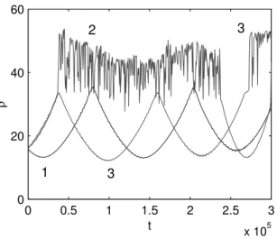
Figures 8 and 9 show the time evolution of ρ and vz for two waves propagating at an angle
of 45◦ (k
iz = kix = 1) to ~B0. As in the case of two perpendicularly propagating waves, there
is coherent change in ρ. During this coherent evolution vz has small-amplitude fluctuations
around its initial value. In the region where the motion in ρ becomes stochastic so does the motion in vz. The stochastic region in vz agrees with the estimate given above. Since ¯vz is
a constant during the coherent motion, the fluctuations in vz are due to the transformation
between ¯vz and vz.
The main effect of equal parallel wavenumbers is to slightly decrease the range of coherent motion from what it is for perpendicularly propagating waves, thus inhibiting some ions from reaching the stochastic region. Numerical studies indicate that |S0x/S0z| and |S−x/S−z| are
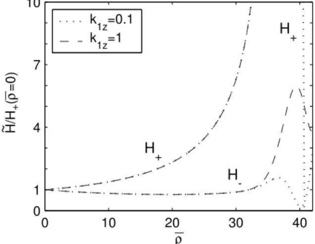
both unity for ξ < 1 but approach 0 as ξ → 1. This raises the bump in H−as kiz is increased.
Consequently, more ions are reflected by H−and the range of coherent motion in ρ is slightly
Figure 11 shows the range of motion ξmin, ξmax for different k1z. Increasing kiz slightly lowers
ξmax since the enhanced bump in H− reflects more ions. Generally then, significant coherent
energization and access to the stochastic region is obtainable with oblique waves provided that ∆kz = 0, while the normalized kz may be large.
B. Unequal Parallel Wavenumbers: ∆kz 6= 0
When the parallel wavenumbers of the two waves are different, the coherent motion of the ions changes drastically. In this case vz undergoes coherent motion and the term 12v¯z2 in
˜
H (17) is no longer a constant. This limits the range in ρ as ∆kz is increased. Figures 12
and 13 show the time evolution of ρ and vz for the exact orbits obtained from (5) with
k1z = 0.001 and k2z = 0. These figures illustrate the limits in ρ.
Figure 14 shows the variation of H± and 12v¯z2 as functions of ¯ρ. For ¯ρ far from ¯ρ0 = 17,
H+− H−= 2|S−| ¿ 12v¯z2 so that H+ ≈ H−. Figure 15 shows the limitation on the range of
coherent motion in ξ for ∆kz 6= 0.
The coherent motion in vz has the effect of detuning the waves from exact resonance.
The resonance condition for an ion with vz 6= 0 is
R ≡ ν10− ν20− (∆kz)vz ∈ Z (26)
where ν10 and ν20 are the wave frequencies in the laboratory frame, and νi = νi0 − kizvz.
˜
H describes the ion’s motion as long as R is close to an integer. For ∆kz 6= 0, vz changes
coherently. Condition (26) is not satisfied for all times, and the resonant interaction becomes less effective. The coherent change in vz thus limits itself, which keeps R close to an integer.
Since the coherent changes in ¯ρ and ¯vz are linked via (19), the coherent change in ¯ρ is also
small.
Consider a distribution of ions with different initial vz0 interacting with two waves of
frequencies ν10 and ν20. For ∆kz = 0, all ions will be in resonance with the waves provided
ν10− ν20∈ Z. For ∆kz 6= 0, the resonance condition (26) implies that only ions with certain
vz0, namely
vz0 ≈
ν10− ν20− n
∆kz
, n ∈ Z (27)
are initially in resonance. As vz changes coherently, they fall out of resonance.
This situation is analogous to the case of two perpendicularly propagating waves when the wave frequencies do not differ by an integer [12]. Following Section IV.C of [12], the approximate Hamiltonian, correct to second order in wave amplitudes, that describes the coherent motion is
˜
Hof f = −
∆ν
N I + ˜¯ H (28)
where (ν1− ν2) = N + ∆ν and |∆ν| ¿ 1. In this case the barriers H± are given by
H± = −
∆ν N I +¯
1
2v¯z2+ S0± |S−| (29)
The first term in (28) limits the coherent motion, and plays a similar role to 1
2v¯z2. Figure 16
shows the range of motion in ξ as a function of ∆ν. the largest range of coherent motion occurs for ∆ν slightly different from 0, which allows −(∆ν/N) ¯I to partly cancel S0 in
As the wave frequencies are increased, the range in ∆kz and ∆ν for which there is
appre-ciable coherent motion becomes much narrower. Let ξa(∆kz) be either the upper or lower
bound of coherent motion in ξ for wave frequencies ν1a and ν2a = ν1a− N. The asymptotic
forms in Appendix B indicate that for two different frequencies ν1b and ν2b = ν1b− N,
ξb(∆kz) ≈ ξa õ ν1b ν1a ¶3 ∆kz ! (30) Suppose ξa is large for k1 ≤ ∆kz ≤ k2, and that ν1b = 4ν1a. Then ξb is large only for
k1/64 ≤ ∆kz ≤ k2/64. Coherent motion occurs over a smaller range of ∆kz when the wave
frequencies are larger. Similarly,
ξb(∆ν) ≈ ξa õ ν1b ν1a ¶4 ∆ν ! (31) Figures 15 and 16 demonstrate the range of coherent motion versus ∆kzand ∆ν, respectively,
and validate the scalings in (30) and (31) with wave frequency. As the wave frequencies are increased, ∆kz and ∆ν must be much smaller for ions to be energized to the stochastic
region. Hence, just as in the cases of perpendicular propagation or ∆kz = 0, for nonzero but
small ∆kz energization by waves with low frequencies is more advantageous than by waves
with high frequencies.
VI. CONCLUSIONS
We have shown that two electrostatic waves propagating obliquely to an ambient mag-netic field can coherently energize ions when their Doppler-shifted frequencies differ by a multiple of the ion cyclotron frequency. A second-order Hamiltonian, derived using the Lie perturbation technique, accurately describes the coherent motion and agrees well with nu-merical simulations of the complete dynamical equations. The energization of ions occurs regardless of the angle of wave propagation provided the parallel wavenumbers of the two waves are approximately equal. If the parallel wavenumbers are equal, there is no coherent acceleration along ~B0 but considerable stochastic energization both along and across ~B0.
Moreover, the perpendicular coherent motion is quite similar to the case of perpendicularly propagating waves. There is a small amount of coherent acceleration along ~B0 when the
parallel wavenumbers differ, but this causes the resonance condition to be violated. A dif-ference between the parallel wavenumbers is similar to the difdif-ference between (ω1− ω2)/ωci
and the nearest integer.
There is no threshold ion energy or wave amplitude required for the coherent acceleration. The change in the ion gyroradius is linear in the wave frequencies and independent of wave amplitude. The period of coherent motion is inversely proportional to the square of the wave amplitudes and is proportional to the fourth power of the wave frequency ω (ω ∼ ω1 ∼ ω2).
Furthermore, the deviation from resonance ∆ω = ω1 − ω2 − Nωci for which appreciable
coherent acceleration occurs scales like ω−4, while the range in ∆k
z = k1z− k2z for coherent
motion scales like ω−3. This implies that for lower-frequency waves coherent ion acceleration
is faster and less sensitive to small changes in wave parameters.
Coherent ion energization occurs for two waves with appropriately chosen frequencies. An experiment is being constructed that will be able to test the theoretical predictions of
this paper [21]. Coherent acceleration could also occur for a broadband spectrum of waves extending over at least two ωci in frequency. Such a situation can occur naturally in the
Earth’s ionosphere [13]. Detailed analyses of a broad spectrum of waves, and of the effects of weak collisions, remain to be carried out in future work.
Acknowledgments
The authors thank Prof. A. Brizard for helpful discussions on the Lie transforma-tion technique. We also appreciate enlightening comments from Dr. D. B´enisti about his work on this problem. We thank R. Spektor for discussing his work with us and ex-ploring possible experimental realizations of this process. This work was supported by DOE Contract DE-FG02-91ER-54109, DOE/NSF Contract DE-FG02-99ER-54555, NSF Contract ATM-0114462, and Princeton University Subcontract 150-6804-1. DJS was partly supported by an NDSEG Graduate Fellowship.
APPENDIX A: LIE PERTURBATION METHOD FOR TWO OBLIQUE WAVES
We develop the Lie perturbation method following Refs. [18] and [17] and follow the notation in Section 2.5 of Ref. [18].
The Lie method provides a Hamiltonian ¯H that describes just the coherent motion, and a change of coordinates that accounts for the incoherent fluctuations. The physical variables x = (q, p) are governed by the full Hamiltonian H(x), and the new coordinates ¯x = (¯q, ¯p) are governed by ¯H(¯x). ¯x depends on x and a parameter ² which orders the perturbation via
∂ ¯x
∂² = [¯x, w(¯x, t)]x¯, x(² = 0) = x¯ (A1) where [f, g]x =
P
i[(∂f /∂qi)(∂g/∂pi) − (∂f /∂pi)(∂g/∂qi)] is the Poisson bracket. The old
coordinates enter only as a condition for ² = 0, which ensures that the transformation for any w is canonical and near-identity.
The operator T relates the representation of a physical quantity f in the two coordinate systems by f (¯x) = (T f )(x). In particular, f (¯x) = ¯x gives ¯x = T x. T satisfies
∂T ∂²f (x) = −T [w(x, t), f (x)]x (A2) ¯ H is given by ¯ H(¯x) = T−1H(x) + T−1 Z ² 0 d²0T (²0)∂w(x, t) ∂t (A3)
The second term is not needed for an autonomous system.
We expand w, H, T, and ¯H in powers of ² and equate terms at each order in ². Collecting terms in (A3) at each order in ² gives equations for wi. Upon carrying out the perturbation
expansion to second order in ², we find
D0w1 = ¯H1− H1 (A4)
D0f ≡ ∂tf +[f, H0] is the time derivative along the unperturbed trajectories. All expressions
here are functions of the same set of coordinates. For simplicity we use x for this purpose, but the final expression for ¯H governs the evolution of ¯x. Clearly, ¯H0 = H0.
For T to be a near-identity operator, w must remain small. We choose ¯Hi in the
right-hand side of (A4) and (A5) to eliminate any terms that would violate this condition. Such terms are referred to as “resonant” terms.
For the two-wave problem, H0 and H1 are given in (7), while Hi = 0 for i ≥ 2. Using a
Bessel-function identity (see p. 361 of [22]), we obtain H1 = X i ∞ X m=−∞
²iJm,icos ψmi (A6)
where Jm,i ≡ Jm(kixρ) and ψmi ≡ mφ + kizz − νit + αi. Then from (A4)
(∂t+ ∂φ+ vz∂z)w1 = ¯H1−
X
i,m
²iJm,icos ψmi (A7)
The unperturbed orbits are φ = t + φ0, z = z0, vz = 0, I = I0 (in a frame where the ion’s
initial vz0 = 0). Along these orbits there are no resonant terms on the right-hand side of
(A7), so we choose ¯H1 = 0. Then
w1 = − X i,m ²iJm,i m + kizvz− νi sin ψmi (A8)
Since H2 and ¯H1 are zero, (A5) leads to
(∂t+ ∂φ+ vz∂z)w2 = 2 ¯H2− [w1, H1] (A9) From (A8) [w1, H1] = X i,j,m,n n²i²j 2ρ 1 m − µi
(−kjxmJm,iJn,j0 + kixnJm,i0 Jn,j) cos Γ+
+²i²j 2ρ
1 m − µi
(−kjxmJm,iJn,j0 − kixnJm,i0 Jn,j) cos Γ−
+1 2²i²jkizkjz Jm,iJn,j (m − µi)2 (− cos Γ++ cos Γ−) o (A10)
where Γ± ≡ ψmi± ψnj. Along the unperturbed orbits, Γ± = {m − νi± (n − νj)}t + const.
Some terms are resonant when i = j regardless of the νi’s. Other terms are resonant when
either 2νi, N+ ≡ (ν1+ ν2), or N ≡ (ν1− ν2) is an integer. We construct ¯H2 to cancel these
terms: ¯
H2 = S0(I, vz) + δ−S−(I, vz) cos((ν1− ν2)(φ − t) + (k1z− k2z)z + α1− α2)
+ δ+S+(I, vz) cos((ν1+ ν2)(φ − t) + (k1z+ k2z)z + α1+ α2)
+X
i
δiSi(I, vz) cos(2νi(φ − t) + 2kizz + 2αi)
where δ−, δ+, and δiare unity when, respectively, N, N+, and 2νiare integers and 0 otherwise.
Equations (10) and (13) give S0 and S−, and
S+ = − X m n ² 1²2 4ρ(m − µ1) (k1x(m − N+)Jm,10 J−m+N+,2+ k2xmJm,1J 0 −m+N+,2) +1 4k1zk2z²1²2 Jm,1J−m+N+,2 (m − µ1)2
+ the same with subscripts 1 and 2 switched o (A12) Si = − X m n ²2 i 4ρ(m − µi) (mkixJm,iJ−m+2ν0 i,i+ (m − 2νi)kixJ 0 m,iJ−m+2νi,i) +1 4²2ik2iz Jm,iJ−m+2νi,i (m − µi)2 o (A13) The coherent Hamiltonian is
¯
H(¯x, t) = H0(¯x) + ¯H2(¯x, t) (A14)
Using ¯ψ = ¯φ − t as the coordinate conjugate to ¯I, the transformed Hamiltonian is ˜
H( ¯ψ, ¯z, ¯I, ¯vz) = 21v¯2z+ ¯H2 (A15)
˜
H is a constant of the motion.
When only one resonance condition is satisfied, we find a second constant of the motion besides ˜H, which relates ¯I and ¯vz (when only N is an integer, this constant is ¯vz−(∆kz/N) ¯I).
The dynamical system described by (A15) is thus completely integrable. When any two resonance conditions are satisfied it is easy to see that ν1 and ν2 must both be half-integers.
Then all four resonance conditions are satisfied. It does not appear that, in this case, there exists a second constant of the motion. The dynamics described by ˜H could be stochastic.
To find the transformation relating x and ¯x, we expand (A2) and use ¯x = T x. To first order in ² we obtain
¯
x = T x ≈ x − ²[w1(x, t), x]x+ O(²2) (A16)
As desired, the coordinate change is near-identity. The relation between I and ¯I is given in (16).
APPENDIX B: ASYMPTOTIC FORMS FOR S0 AND S−
Here we derive the asymptotic forms for the terms in ˜H, given in (17), using results in Refs. [5, 22–24]. For k1x= k2x = 1, let
S0x = 2 X i=1 ²2 isx(ρ, µi, 0) (B1) S−x = ²1²2(sx(ρ, µ1, N ) + sx(ρ, µ2, −N)) (B2) S0z = 2 X i=1 k2 iz²2isz(ρ, µi, 0) (B3) S−z = ²1²2k1zk2z(sz(ρ, µ1, N ) + sz(ρ, µ2, −N)) (B4)
where sx(ρ, µ, n) = (−)n π 8 csc µπ(Jµ+1J−(µ+1)+n− Jµ−1J−(µ−1)+n) (B5) sz(ρ, µ, n) = (−)n+1 π 4 ∂ ∂µ[csc µπJµJ−µ+n] (B6) and Jµ= Jµ(ρ).
Bessel functions of negative order are replaced with
J−µ≈ − sin(µπ)Yµ (B7)
where Yµ is the Bessel function of the second kind. Using the asymptotic forms for Jµ and
Yµ [22], we obtain σ(µ, ρ, n) ≡ Jµ(ρ)Yµ−n(ρ) ∼ βeγ (B8) β = −1 π(µ(µ − n) tanh α0tanh αn) −1/2 (B9) γ = µ(tanh α0− α0) − (µ − n)(tanh αn− αn) (B10) sech αn = ρ µ − n (B11)
For N + 1 ¿ µ all the n/µ’s are small, and to leading order in n/µ we find β ≈ − 1 µπ(1 − ξ 2)−1/2 (B12) γ ≈ −nα0 (B13) σ ≈ − 1 µπσ0(ξ, n) (B14) σ0(ξ, n) ≡ (1 − ξ2)−1/2 Ã ξ 1 +p1 − ξ2 !n (B15) Thus, sz ≈ π 4 ∂ ∂µσ(µ, ρ, n) (B16) ≈ f (ξ, n) µ2 (B17) f (ξ, n) ≡ 1 4 µ σ0+ ξ ∂σ0 ∂ξ ¶ (B18) Similarly, sx ≈ π 8(σ(µ + 1, ρ, n) − σ(µ − 1, ρ, n)) (B19) ≈ π 8(σ1(²) − σ1(−²)) (B20) σ1(²) = σ0(ξ/(1 + ²), n) µ(1 + ²) (B21)
where ² ≡ 1/µ is small for µ À 1. Expanding σ1 to leading order in ², sx ≈ π 4²σ 0 1(0) (B22) = f (ξ, n) µ2 (B23) Thus, sx ≈ sz ∼ 1 µ2 (B24)
[1] C. F. F. Karney and A. Bers, Physical Review Letters 39, 550 (1977). [2] C. F. F. Karney, Physics of Fluids 21, 1584 (1978).
[3] G. M. Zaslavsky, R. Z. Sagdeev, D. A. Usikov, and A. A. Chernikov, Weak Chaos and
Quasi-Regular Patterns (Cambridge University Press, Cambridge, UK, 1991).
[4] A. Fukuyama, H. Momota, R. Itatani, and T. Takizuka, Physical Review Letters 38, 701 (1977).
[5] P.-K. Chia, L. Schmitz, and R. W. Conn, Physics of Plasmas 3, 1545 (1996). [6] G. R. Smith and A. N. Kaufman, Physics of Fluids 21, 2230 (1978).
[7] G. R. Smith and A. N. Kaufman, Physical Review Letters 34, 1613 (1975). [8] L. Chen, Z. Lin, and R. White, Physics of Plasmas 8, 4713 (2001).
[9] J. M. McChesney, P. M. Bellan, and R. A. Stern, Physical Review Letters 59, 1436 (1987). [10] S. Benkadda, A. Sen, and D. R. Shklyar, Chaos 6, 451 (1996).
[11] A. K. Ram, A. Bers, and D. B´enisti, in Eos Transactions of the American Geophysical Union,
Fall Meeting (1997), vol. 78.
[12] D. B´enisti, A. K. Ram, and A. Bers, Physics of Plasmas 5, 3224 (1998).
[13] A. K. Ram, A. Bers, and D. B´enisti, Journal of Geophysical Research [Space Physics] 103, 9431 (1998).
[14] A. K. Ram, L. Kang, and A. Bers, in Eos Transactions of the American Geophysical Union,
Fall Meeting (1998), vol. 79.
[15] H. Goldstein, Classical Mechanics (Addison-Wesley, Reading, Mass., 1980), 2nd ed.
[16] W. H. Press, B. P. Flannery, S. A. Teukolsky, and W. T. Vetterling, Numerical Recipes (Cambridge University Press, Cambridge, UK, 1986).
[17] J. R. Cary, Physics Reports 79, 129 (1981).
[18] A. J. Lichtenberg and M. A. Lieberman, Regular and Chaotic Dynamics (Springer-Verlag, New York, NY, 1992), 2nd ed.
[19] D. B´enisti, A. K. Ram, and A. Bers, Physics of Plasmas 5, 3233 (1998). [20] D. B´enisti, A. K. Ram, and A. Bers, Physics Letters A 233, 209 (1997).
[21] E. Choueiri and R. Spektor, in Bulletin of the American Physical Society (2000), vol. 45(7). [22] M. Abramowitz and I. A. Stegun, Handbook of Mathematical Functions (Dover Publications,
Inc., New York, NY, 1970).
[23] I. S. Gradshteyn and I. M. Ryzhik, Table of Integrals, Series, and Products (Academic Press, New York, NY, 1965), 4th ed.
[24] R. Spektor and E. Y. Choueiri, Ion acceleration by beating electrostatic waves: Domain of
allowed acceleration, Paper IEPC-01-209, 27th International Electric Propulsion Conference,
0 1 2 3 4 5 x 10⁵ 0 20 40 60 80 100 1 2 3 t ρ
FIG. 1: ρ versus t for three ions interacting with two perpendicular waves from the full Hamiltonian
H (5). Quantities in all figures are given in terms of the normalized units defined in the text. The
initial ρ0= 15.95 (ξ0 = ρ0/ν1= 0.4) for all three ions while their phases are φ0= (−0.3, 0.2, 0.4)π
for ions labelled 1, 2, and 3, respectively. The parameters for the two waves are: ²1 = ²2= 4,
k1x= k2x= 1, k1z = k2z = 0, ν1 = 40.37, and ν2 = ν1− 1. 0 0.5 1 1.5 2 x 10⁵ 0 20 40 60 80 100 t ρ
FIG. 2: ρ versus t for the same parameters as in Fig. 1 except that ρ0 = 15.95, 30, 45 and
0 1 2 3 4 5 x 10⁵ 0 10 20 30 40 50 1 2 3 t ρ SR
FIG. 3: ¯ρ versus t from the coherent Hamiltonian ˜H (17) for the same parameters as in Fig. 1. SR
indicates the stochastic region for the full Hamiltonian.
0 10 20 30 40 4 6 8 10 12 14 x 10-3 ρ H H + H + H -2 1 3 ~
FIG. 4: H+ and H− versus ¯ρ for the same parameters as in Fig. 1. The initial values of ˜H for the three ions in Fig. 1 are marked by the open circles.
0 0.2 0.4 0.6 0.8 1 0 1 2 3 4 5 6 ξ H/H + (ξ =0) H -H+ ν 1=10.37 ν 1=70.37 H + ~
FIG. 5: H±/H+(ξ = 0) versus ξ ≡ ¯ρ/ν1 for N = 1 and ν1 = 10.37 (solid line) and ν1 = 70.37
(dashed line). ²1 = ²2=arbitrary, k1x= k2x= 1, and k1z = k2z = 0.
0 20 40 60 80 0 0.2 0.4 0.6 0.8 1 ν1 ξ ξmax ξmin
FIG. 6: Average ξmin and ξmax versus ν1 for perpendicularly propagating waves based on the
barriers H±. Parameters are as in Fig. 5 except that ν1 = (3.37, 4.37, ..., 80.37), ξ0 = 0.4, and the
0 20 40 60 80 0 1 16 81 256 625 1296 ν 1 τ x104 φ 0=0.2π φ 0=0.6π
FIG. 7: The period of coherent oscillation τ versus ν1. The other wave parameters are the same as
in Fig. 1. The initial conditions are ξ0 = 0.4 and φ0 = (0.2, 0.6)π. The open circles and stars are
the periods obtained from integrations of the dynamics given by ˜H. The solid lines are proportional
to ν4
1 with the constant of proportionality chosen to match the period at ν1= 40.37. The vertical
axis is scaled so that ν4
1 is a straight line. 0 0.5 1 1.5 2 2.5 3 x 10⁵ 0 20 40 60 t ρ 1 3 2 3
0 0.5 1 1.5 2 2.5 3 x 10⁵ 20 0 20 40 60 80 t v z 1 3 2
FIG. 9: vz versus t for the same parameters as in Fig. 8.
0 10 20 30 40 0 1 4 7 10 ρ H/H + (ρ =0) H+ H -k 1z=0.1 k 1z=1 H + ~
FIG. 10: H±/H+(¯ρ = 0) versus ¯ρ for k1z = k2z = 0.1 (dots) and 1 (dashes). Other parameters are
as in Fig. 8. The curves for k1z = 0 are very close to those for k1z = 0.1.
10-3 10-2 10-1 100 101 0 0.2 0.4 0.6 0.8 1 k 1z ξ ξmax ξmin
FIG. 11: Average ξmin and ξmax versus k1z for k2z = k1z from H±. ν1 = 40.37 and the other
0 1 2 3 x 10⁵ 0 10 20 30 t ρ 2 1 3
FIG. 12: ρ versus t for the same parameters as in Fig. 1 except that k1z = 0.001 and k2z = 0.
0 0.5 1 1.5 2 2.5 3 x 10⁵ 0.1 0 0.1 t v z 1 2 3
FIG. 13: vz versus t for the same parameters as in Fig. 12.
6 10 14 18 22 0 5 10 15 20 x 10-3 ρ H H + H -v z 2 /2 ~ FIG. 14: H± and 1
-4 -3 -2 -1 10 10 10 10 100 0 0.2 0.4 0.6 0.8 1 ∆ k for ν =10.37 ξ ν 1=10.37 ν 1=40.37 10 10 10 10 100 0 0.2 0.4 0.6 0.8 1 ∆ kz for ν1=10.37 ξ ν 1=10.37 ν 1=40.37 10-5 10-4 10-3 10-2 0 0.2 0.4 0.6 0.8 1 ∆ k z for ν1=40.37
FIG. 15: Average ξmin and ξmax versus ∆kz from H± for k1z = 0.1, k2z = k1z− ∆kz, ν1 = 10.37
(dotted) or 40.37 (dashed), and the other wave parameters as in Fig. 1. Initial conditions and averaging are as in Fig. 6. The abscissa for ν1 = 40.37 has been rescaled by (10.37/40.37)3. If the
scaling in (30) were exact, the dotted and dashed lines would coincide.
0.1 0.05 0 0.05 0.1 0 0.2 0.4 0.6 0.8 1 1.2 ∆ ν for ν1=10.37 ξ ν1=10.37 ν1=40.37 0.1 0.05 0 0.05 0.1 0 0.2 0.4 0.6 0.8 1 1.2 ∆ ν for ν1=10.37 ξ ν 1=10.37 ν1=40.37 4 2 0 2 4 x 10⁻⁴ 0 0.2 0.4 0.6 0.8 1 ∆ ν for ν1=40.37
FIG. 16: Average ξmin and ξmax versus ∆ν from H± for ν2 = ν1− 1 − ∆ν, ν1 = 10.37 (dotted) or
40.37 (dashed) and the other wave parameters as in Fig. 1. Initial conditions and averaging are as in Fig. 6. The abscissa for ν1 = 40.37 has been rescaled by (10.37/40.37)4. If the scaling in (31)